

CNN-BiLSTM: A Novel Deep Learning Model for Near-Real-Time Daily Wildfire Spread Prediction


1
Department of Electrical and Computer Engineering, Memorial University of Newfoundland, St. John’s, NL A1C 5S7, Canada
2
C-CORE, St. John’s, NL A1B 3X5, Canada
*
Author to whom correspondence should be addressed.
Remote Sens. 2024, 16(8), 1467; https://doi.org/10.3390/rs16081467
Submission received: 11 March 2024
/
Revised: 14 April 2024
/
Accepted: 15 April 2024
/
Published: 20 April 2024
(This article belongs to the Special Issue Advanced Artificial Intelligence for Remote Sensing: Methodology and Applications)
Abstract
:Wildfires significantly threaten ecosystems and human lives, necessitating effective prediction models for the management of this destructive phenomenon. This study integrates Convolutional Neural Network (CNN) and Bidirectional Long Short-Term Memory (BiLSTM) modules to develop a novel deep learning model called CNN-BiLSTM for near-real-time wildfire spread prediction to capture spatial and temporal patterns. This study uses the Visible Infrared Imaging Radiometer Suite (VIIRS) active fire product and a wide range of environmental variables, including topography, land cover, temperature, NDVI, wind informaiton, precipitation, soil moisture, and runoff to train the CNN-BiLSTM model. A comprehensive exploration of parameter configurations and settings was conducted to optimize the model’s performance. The evaluation results and their comparison with benchmark models, such as a Long Short-Term Memory (LSTM) and CNN-LSTM models, demonstrate the effectiveness of the CNN-BiLSTM model with IoU of F1 Score of 0.58 and 0.73 for validation and training sets, respectively. This innovative approach offers a promising avenue for enhancing wildfire management efforts through its capacity for near-real-time prediction, marking a significant step forward in mitigating the impact of wildfires.
1. Introduction
Over the past two decades, the environment has suffered extensive damages amounting to billions of dollars due to devastating wildfires. This destructive phenomenon stands out as among the most severe disasters, inflicting ecological harm and causing casualties among both forests and people [1]. For instance, the 1983 wildfires in Victoria, Australia, resulted in the burning of 392,000 hectares of land and claimed the lives of 75 people [2]. India experienced wildfires affecting 5.7 million hectares of land from 1985 to 1990, with 17,852 reported incidents [3]. In Portugal in 2003, 20 people lost their lives, and 420,000 hectares were destroyed due to wildfires [4]. Spain, in 2006, witnessed the devastation of nearly 150,000 hectares by wildfires [5]. Canada faces an average of 8000 wildfires annually, consuming an average of 2.5 million hectares of land each year [6]. A wildfire in the southeast of Australia in September 2019 burned 11.2 million hectares of forests, leading to the tragic deaths of numerous animals [7]. As the frequency, duration, and intensity of wildfires increase with the impact of climate change, their destructive potential is expected to increase. To mitigate the impacts posed by wildfires on human lives and property, it is imperative to implement management strategies that mitigate these destructive impacts [8].
Early detection and prediction of wildfires can significantly reduce the destructive impact of wildfires [9]. It is essential to acknowledge, however, that complete prevention of wildfires in vegetated areas is not possible. Therefore, a crucial tool for accurately predicting the spread of wildfires across diverse geographies, climates, and fuel types is needed.
Researchers worldwide have actively engaged in wildfire research, recognizing the global significance of the issue. Modeling dynamic processes on the Earth’s surface entails a high degree of uncertainty, as the information is either initially known with some error or undergoes changes over time [10].
Previous studies categorized wildfire spread models into three main types: stochastic, phenomenological, and physical [11]. In a physical model, equations governing combustion, fluid dynamics, and heat transfer are solved to determine the spatio-temporal distribution of wildfires [12,13,14]. Examples of physics-based models, such as Forbes [15] and Wildland–Urban Interface Fire Dynamics Simulator (WFDS) [16], incorporate fuel fundamentals, combustion, and energy transfer. Stochastic wildfire spread models utilize statistics from historical wildfires and prescribed burns. These models summarize wind speed, fuel type, and soil moisture using respective functional forms [17]. Phenomenological wildfire spread models rely on experimental measurements rather than models based on first principles to develop functional forms [18]. One of the widely used models for phenomenological time scales is Rothermel’s model [19]. The abovementioned approaches demand extensive computations at various ignition locations, making it a time-consuming process. For instance, the computational time for a single fire spread simulation could reach 872,000 min (approximately 600 days) on a single processor [20]. Therefore, new approaches are needed to decrease these computational costs.
Recently, the prediction of wildfire spread has witnessed significant improvements through the utilization of machine learning algorithms [21,22,23,24]. These algorithms use observed knowledge of previous wildfire patterns to predict future wildfire fronts [11]. Illustratively, [25] conducted a study to evaluate the efficacy of Random Forest (RF), Logistic Regression (LR), and convolutional autoencoder models in predicting wildfire spread. They used diverse environmental variables acquired through remote sensing technology in their analysis. The outcomes of their research indicated that the Convolutional Neural Network (CNN) model surpasses the others in terms of performance, showcasing a structural superiority that aligns well with the characteristics of the provided data. In a similar work, Marjani and Mesgari (2023) [26] introduced a multi-kernel CNN model that integrated diverse data types such as topographical, meteorological, anthropological, fuel, and hydrological data to predict wildfire spread in the United States. Despite its comprehensive approach, the model faced performance challenges when dealing with large pixel-size data (1 km) in real-world scenarios. Furthermore, both studies did not consider the temporal aspect of wildfires. To cover these gaps, [27] introduced a Convolutional Long Short-Term Memory (ConvLSTM) network to mitigate computational costs associated with predictions. However, their approach involved using simulated data rather than real burn maps as training data. Subsequently, the FirePred [28] model was proposed using actual wildfire datasets, incorporating both spatial and temporal considerations using various temporal blocks in its architecture. Despite these improvements, a notable challenge arose in real-world scenarios where FirePred struggled to predict future burned maps due to its reliance on initial burn maps—a requirement that is not available during the early stages of a wildfire. The studies mentioned share a common limitation as they rely on an initial burn map from the previous time step to predict wildfire spread in the next steps. In real-world scenarios, the absence of this initial map poses a significant challenge. Therefore, there is a pressing need for additional research to explore innovative approaches that can effectively address this critical gap in existing methodologies.
To cover the mentioned limitations, this study introduces a novel approach by proposing a hybrid model, CNN and Bidirectional Long Short-Term Memory (BiLSTM) components, referred to as the CNN-BiLSTM model. This model addresses the challenges associated with spatial and temporal patterns in wildfire spread prediction, using Visible Infrared Imaging Radiometer Suite (VIIRS) active fire data as a near-real-time source for generating initial burn maps. The primary contributions of this study include (1) the development of the CNN-BiLSTM model designed for near-real-time wildfire spread prediction, (2) the integration of both spatial and temporal considerations into the wildfire spread prediction task through the fusion of CNN and BiLSTM modules, and (3) analysis of the influences of environmental parameters on the model predictions.
2. Materials and Methods
2.1. Study Area
The research is conducted in Laura, Queensland, Australia, a region known for its substantial rainforest expanses and diverse biological landscapes, featuring 226 national parks. The climate in this area is characterized by hot and humid summers, along with warm and dry winters. The region encounters recurring threats of droughts and bushfires. According to data from the Global Fire Emissions Database (GFED), this particular area experienced the second-longest recorded fire in history until 2016 [29,30]. The wildfire persisted for an extensive period, raging from 13 September 2015 to 12 December 2015, spanning a total of 91 days. Figure 1 shows the extent of the study area.
2.2. Dataset
In this study, we employed the VIIRS dataset [31] for the specified date. This dataset includes point shapefiles representing active fires on given dates, which are available for daily access. Meteorological data used in this study include precipitation, soil moisture, and runoff. These daily data were collected from the Australian Landscape Water Balance (ALWB) (https://awo.bom.gov.au/products/ (accessed on 22 September 2021)) between 13 September 2015 and 12 December 2015. Moreover, the daily aggregated temperature was collected from the European Centre for Medium-Range Weather Forecasts (ECMWF) Reanalysis v5 (ERA-5) (https://cds.climate.copernicus.eu/cdsapp#!/dataset/reanalysis-era5-land?tab=overview (accessed on 12 February 2024)) with the spatial resolution of using the Google Earth Engine (GEE) platform. It is recognized that the intensity and spread of a wildfire can be mitigated by increased values of each of these variables. Additionally, the wind speed and direction data obtained from the nearest weather station to Laura were incorporated into the dataset (https://mesonet.agron.iastate.edu/request/daily.phtml# (accessed on 22 September 2021)).
Land cover and vegetation characteristics are important elements in determining wildfire spread dynamics. Certain plant species are highly sensitive to wildfire, and areas devoid of vegetation are less prone to wildfire spread. To consider this information, we utilized the Normalized Difference Vegetation Index (NDVI) and land cover data. The 2015 land cover data, created by the European Space Agency (ESA) for long-term and consistent climate modeling, categorizes the study area into six classes: (1) tree cover—broadleaved, evergreen, closed to open (>15%); (2) tree cover—broadleaved, deciduous, closed to open (>15%); (3) tree cover—broadleaved, deciduous, open (15–40%); (4) mosaic tree and shrub (>50%) and herbaceous cover (<50%); (5) shrubland; and (6) deciduous shrubland.
NDVI data were obtained using the Terra Moderate Resolution Imaging Spectroradiometer (MODIS) sensor called MOD13Q1. These data are generated every 16 days as Level 3 products with a spatial resolution of 250 m (m). Furthermore, we considered earth surface characteristics that influence wildfire spread, including elevation, slope, and aspect. Elevation data were collected from the Shuttle Radar Topography Mission (SRTM) with a 30 m resolution. Slope and aspect data were derived from the elevation data using the Quantum Geographic Information System (QGIS) software (version 3.32.3) by calculating the angle of inclination to the horizontal. Table 1 indicates an overview of datasets used in this study for wildfire spread prediction.
2.2.1. Data Preparation
The daily wildfire data, acquired from the sensor at a specific time, exhibits movement throughout the day rather than remaining static. As the sensor revisits the area the next day, any new fires are detected. Given the current limitations of sensor technology, which cannot provide temporal resolution finer than a day, a method is required to estimate the burned in a day. This challenge is addressed by employing a fixed radius and the density of points per day. The Global Fire Emissions Database (GFED) provides the average rate per day of fire spread in the area. Equation (1) calculates the constant value of the radius by considering time, which is 24 h.
In Equation (1), represents the average rate of wildfire spread, and is time. The radius obtained from Equation (1) is then utilized to calculate the density of points. Finally, we used a constant 95th percentile threshold value to extract the estimated burned area for each day from the density analysis output.
Land cover data are typically classified as categorical data, where each class is assigned a unique number. To eliminate the hierarchical nature of these numbers, one-hot encoding is applied. Given the six classes of land cover in the study area, a binary map is generated for each class, assigning a value of one where the desired class exists and zero otherwise.
Considering the limited temporal resolution of available data sources, NDVI is not available for all 91 days of the wildfire. To address this, interpolation is performed for days without NDVI. A procedure is applied where NDVI data over a 16-day time step are combined to calculate NDVI for the second day, using the previous day’s NDVI data (when available) except for pixels burned on that day. For these burned pixels, NDVI is obtained from the next available data. This process is repeated for days without NDVI data.
To collect wind direction and speed data, the two nearest weather stations to the study area are utilized. These stations report daily wind directions and speeds. The weighted average of the values reported by these stations is used to determine wind direction and speed for each pixel. The distance of each pixel from the weather stations is calculated, and the inverse distance is employed to weigh the speed and direction values of the stations. Equation (2) illustrates the wind speed calculation for each pixel, with a similar approach for wind direction.
In Equation (2), represents the wind speed in the i,j pixel, is the inverse distance between the i,j pixel and the first station, is the wind speed reported by the first station, is the inverse distance between the i,j pixel and the second station, and is the wind speed reported by the second station.
2.2.2. Data Resampling and Normalization
In this phase, two preprocessing steps are uniformly applied to all the data, given their diverse sources. Since the spatial resolution of the data varies due to its derivation from different sources, each of the predictor variables on each day was resampled to the spatial resolution of 150 m with the nearest neighbor technique [32] to create a consistent daily 150 m resolution dataset. In terms of temporal resolution, GEE and ALWB provide aggregated daily products that are aligned with the requirements of this study.
Considering the extensive range of values in the dataset, potential computational complexity, and challenges in prediction [1], normalization is essential to ensure that all variables carry equal weight. Min–max scaling [33] is employed for this purpose, transforming the original variable ranges through a linear transformation. The min–max formula, depicted in Equation (3), quantifies this scaling process:
where Z represents the output variable, denotes the variables, and min and max stand for the minimum and maximum values, respectively. This normalization ensures that each variable contributes equally to the analysis.
2.2.3. Patch Extraction
The burned area maps and environmental variables for the study area were collected with a daily temporal resolution. For each day, a data cube was created with dimensions of 250 × 400 × 17, where 250 and 400 represent the width and height, respectively, and 17 denotes the number of channels. Due to the substantial size of these data cubes, processing them in their entirety proved to be time-intensive. Consequently, each cube was subdivided into multiple patches along both the x and y dimensions, resulting in a new shape of 50 × 50 × 17. To maintain interaction between patches, a 50% overlap was applied in both the x and y directions during patch extraction (see Figure 2C). Subsequently, to preserve the chronological order of the patches, the data were transformed into a tensor with a shape of 4 × 50 × 50 × 17. In this context, the time step represents the number of occurrences in each sample, with 4 designated as the time step value. Therefore, given a series of five tensors, the model will predict the next occurrence (fifth). Figure 2 visually illustrates the process of patch extraction and the resulting data structure in this study. In total, 1650 patches were extracted using this approach for all 92 days. To prevent an imbalance in the dataset, only the patches containing at least one active fire pixel (within label data) were chosen. Subsequently, this set was partitioned into two new sets, with a validation set accounting for 20% of the samples and a training set including the remaining 80% of samples.
2.3. Time Distributed CNN (TD-CNN)
Recurrent Neural Networks (RNNs) are well-suited for solving time series tasks, while CNNs are effective for extracting features from complex datasets [34]. The main focus of CNNs is to identify spatial features in a single input image. However, certain tasks, such as predicting video processing, involve multiple images presented chronologically to identify movements and directions. To address this, the TD-CNN approach was employed.
The input for TD-CNN is a 5D tensor consisting of samples, time steps, width, height, and channels. The fundamental concept behind TD-CNNs is to apply a standard CNN architecture independently to each time step of the input sequence. This means that the same set of convolutional filters and pooling operations are applied to each time step, enabling the network to capture both spatial and temporal patterns. Figure 3 illustrates the process of the TD-CNN approach.
2.4. Dilated CNN (DCNN)
The wildfire spread prediction is similar to the image segmentation task. The concept of an image pyramid was introduced to enhance segmentation precision [35]. In this pyramid-based approach, features are extracted from various scales, and subsequently, they are interpolated and merged. However, extracting features separately for each scale can increase the network’s size and potentially lead to overfitting [36]. To overcome these limitations, the DCNNs were introduced. This approach inserts holes between pixels with a rate called the dilation rate (DR). By adjusting the DR of an atrous convolutional kernel, varying receptive fields can be achieved. This mechanism can address the diverse shapes and sizes of wildfires, especially those of different sizes.
2.5. Bidirectional LSTM (BiLSTM)
LSTM, known for its efficacy in capturing long-term temporal dependencies [37], comprises two fundamental components: a memory cell capable of preserving its state over time and gating units that regulate the flow of information. The LSTM architecture includes three gates within its elemental cell structure: input, output, and forget. For a given time series where ∈ , the LSTM unit updates according to the following formal expressions:
Here, , , and denote the input gate, output gate, and forget gate, respectively. represents the hidden state at time t with size q over the entire hidden state. The weight matrices , , , ∈ , and biases , , , ∈ are integral components. The sigmoid function, denoted by , and × representing the element-wise multiplication operator, contribute to the formal expressions.
BiLSTM is an extension of the traditional LSTM architecture that enhances the model’s ability to capture temporal dependencies by processing input sequences in both forward and backward directions [38]. In a standard LSTM, information flows only in one direction, from past to future. However, BiLSTM introduces a bidirectional approach, allowing the model to consider past and future contexts simultaneously.
In a BiLSTM, the network is split into two components: one processes the input sequence in the forward direction, while the other processes it in the backward direction. Each component has its own set of memory cells and gates. The forward and backward hidden states at each time step are then concatenated or combined to provide a more comprehensive understanding of the input sequence.
2.6. CNN-BiLSTM Architecture
The proposed CNN-BiLSTM model, illustrated in Figure 4, processes a tensor input with dimensions 50 × 50 × 17 for each time step. The model uses two convolution layers with filter sizes of 64 and 128, followed by a DCNN module with DRs of 1, 3, 6, 12, and 18, all using a consistent filter size of 64. Extracted features are concatenated along the channel axis, followed by a pair of CNN and max-pooling operations with filter sizes of 16 and 32 and kernel sizes of 1 and 3, respectively. Next, the batch normalization layer normalizes the extracted features, which are then flattened in preparation for three BiLSTM layers with 16, 32, and 64 neurons. The output from the last BiLSTM layer is processed through a dense layer with 32 neurons, followed by a final dense layer with 2500 neurons and a sigmoid activation function, determining the burn probability for each pixel in the next time step. A reshape layer transforms the output vector into a 2D map with the shape of 50 × 50 × 1. The rectified linear unit (ReLU) activation function is used in the CNN and dense layers, except for the last dense layer, which employs a sigmoid activation function. In this study, an experimental threshold value was employed for post-processing to convert probability values to a binary value.
2.7. Validation Metrics
Evaluation of a wildfire spread model involves the application of various statistical metrics. Precision, recall, F1-score, and Intersection over Union (IoU) were employed in this study for validation analysis and comprehensive model evaluation (Equations (10)–(13)). Figure 5 provides a visual representation of True Positive (TP), False Negative (FN), False Positive (FP), and True Negative (TN). Beyond the mathematical formulation of these evaluation metrics, Figure 6 offers a visual depiction of the fundamental definitions of precision and recall. In this study, the Binary Cross-Entropy (BCE) was employed as the loss function, chosen for its superior performance compared to other loss functions in previous studies [28].
3. Results
3.1. Experimental Settings
The CNN-BiLSTM model was implemented using TensorFlow and the Anaconda platform. The training and validation processes were executed on an Intel i7-10750H 2.6 GHz processor with 16 GB of RAM, supplemented by an NVIDIA GTX 1650 Ti graphics card. Through trial and error in the training phase, a batch size of 2 was determined, and a learning rate of 0.00005 was set for the CNN-BiLSTM model. To prevent overfitting, the early stopping technique was employed. During each epoch, the model’s performance was evaluated on the validation dataset. If the model’s loss during validation was lower than any previously recorded minimum loss, the model’s weights were adjusted accordingly. Ultimately, upon completion of the training process, the most optimal model was preserved.
3.2. Metric Scores of CNN-BiLSTM Model
The evaluation of the CNN-BiLSTM model involved both the training and validation sets, utilizing precision, recall, F1, and IoU metrics, as previously mentioned. Figure 7 provides histograms illustrating the distribution of recall, precision, F1, and IoU scores for the CNN-BiLSTM model across both sets. The graphical representation in Figure 7 visually indicates the metric variations observed in both training and validation sets. The CNN-BiLSTM model exhibited an average IoU of 0.44 and 0.61 for the validation and training sets, respectively. In terms of precision, recall, and F1 metrics, the proposed model demonstrated average values of 0.62, 0.66, and 0.58 for the validation set, compared to 0.72, 0.82, and 0.73 for the training set. Beyond quantitative results, Figure 8 presents 20 qualitative results across validation samples. These results were classified into two classes: good results and poor results based on visual inspection. While there are instances of accurate predictions, the model faced challenges in some scenarios, failing to accurately forecast wildfire spread in the next time step.
3.3. Model Comparison
In this study, the performance of the CNN-BiLSTM model is compared with other state-of-the-art architectures, including LSTM and CNN-LSTM, in the task of predicting wildfire spread based on the validation data. The evaluation metrics, including precision, recall, F1, and IoU, provide knowledge about the model’s effectiveness (see Table 2). For LSTM, the results show a precision of 0.57, recall of 0.61, F1 of 0.59, and IoU of 0.41. The CNN-LSTM model achieved slightly lower metrics with a precision of 0.53, recall of 0.56, F1 of 0.55, and IoU of 0.36. In comparison, the CNN-BiLSTM model outperformed both, exhibiting a precision of 0.62, a recall of 0.66, an F1 of 0.64, and an IoU of 0.53. These results highlight the superior predictive capabilities of the CNN-BiLSTM model in wildfire spread prediction.
4. Discussion
4.1. CNN-BiLSTM Configuration Effects
The output layer of the CNN-BiLSTM model is designed with a sigmoid function, producing a probability mask for wildfire spread, similar to models such as FirePred [28] and Deep Convolutional Inverse Graphics Network (DCIGN) [8M]. To obtain a binary mask indicating burned areas, a post-processing step involves applying a threshold to the probabilistic predictions. The choice of the threshold directly influences the results. In this study, the IoU metric was employed to determine the optimal threshold value. Figure 9 indicates the change of IoU for different threshold values. Evaluation of validation samples across a range of thresholds (0 to 1) revealed the highest IoU value at 0.42. In contrast to [28] and in alignment with [11], the CNN-BiLSTM model with a threshold of 0.42 exhibited improved prediction maps, showcasing its effectiveness in wildfire spread forecasting.
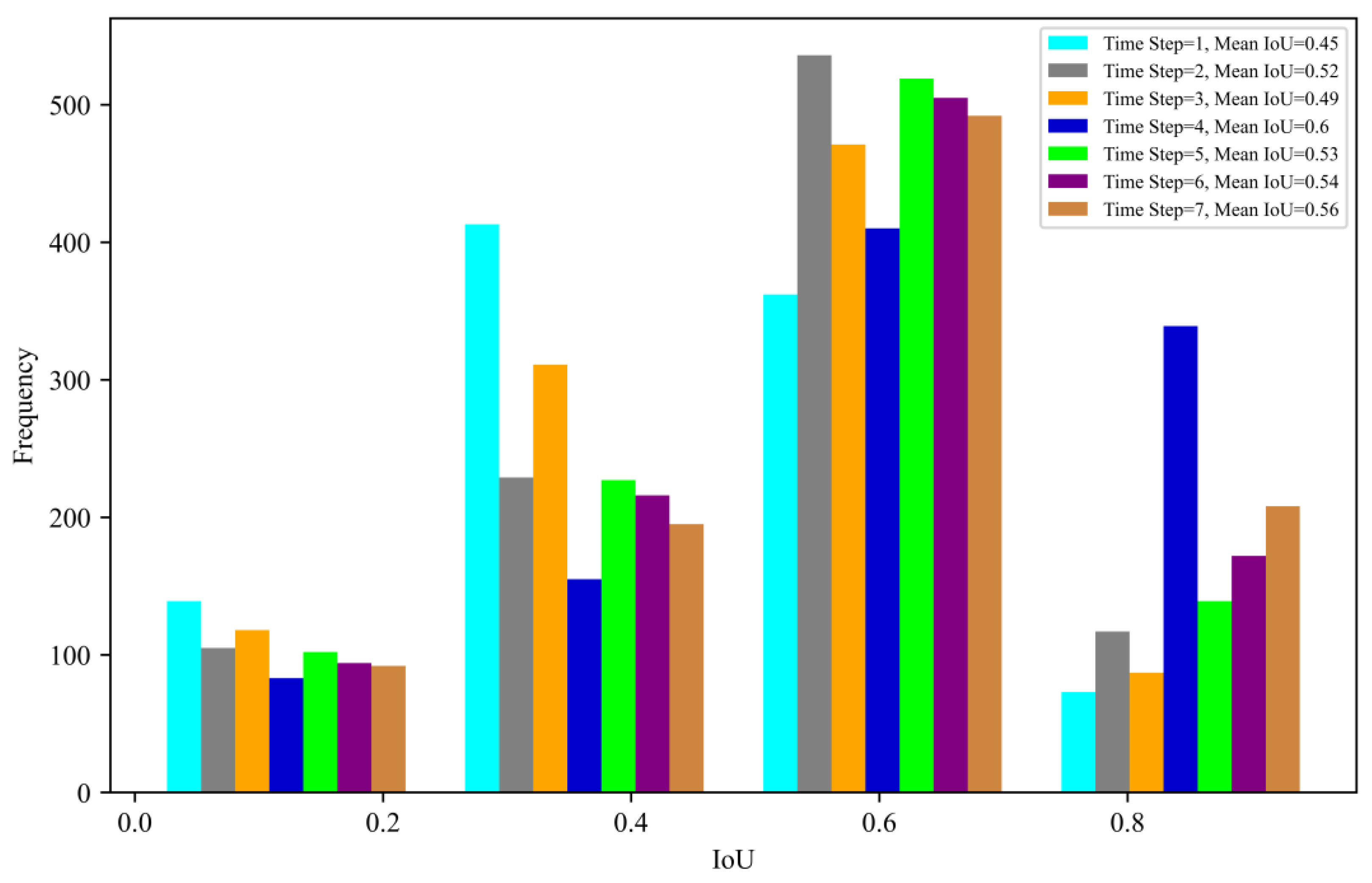
The choice of time step is the next key component that impacts the performance of the CNN-BiLSTM model. To explore its effects, seven different time steps (1 to 7) were assessed, and the trained model was validated with each time step on the validation set. Figure 10 illustrates the IoU histogram for different time steps. Given that the CNN-BiLSTM model considers both spatial and temporal aspects of wildfire, smaller time steps yielded poorer performance. For instance, time steps 1 and 2 resulted in mean IoU values of 0.45 and 0.52, respectively, suggesting the model’s challenge in understanding the spatial–temporal dynamics with shorter time steps. In contrast, larger time steps, like 4 and 5, exhibited a notable increase in performance with mean IoU values of 0.6 and 0.53, respectively. These findings affirm that a larger temporal window enhances the model’s accuracy in predicting wildfire spread. However, an excessive increase in time steps may introduce complexity and compromise results. Therefore, this study opted for a time step of 4 as the optimal time step.
4.2. Environmental Variables and Wildfire Spread
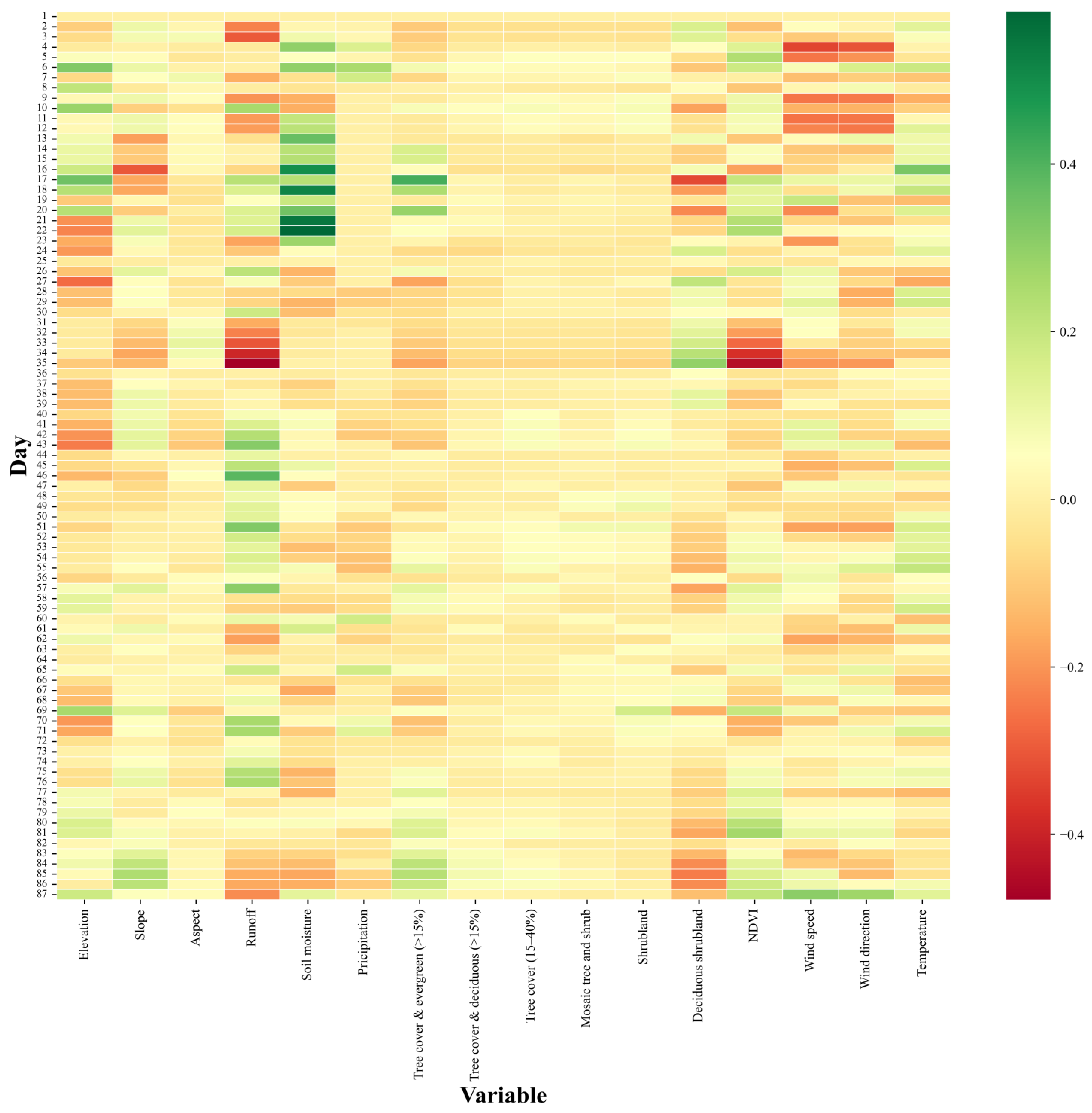
The impact of environmental variables on wildfires, including temperature, runoff, wind vectors, topography, and fuel availability, was investigated through correlation analysis with the CNN-BiLSTM model predictions for each day of the wildfire dataset, as illustrated in Figure 11. Notably, soil moisture exhibited the highest positive correlation between days 21 and 23, ranging from 0.2 to 0.5. Conversely, the lowest negative correlation occurred on the 35th day, specifically for the runoff and NDVI variables. While a positive correlation was expected for NDVI, a few days showed a negative correlation with the CNN-BiLSTM model, potentially attributed to false-positive (FP) predictions. The consistent burnability capability across land cover classes during the study period may contribute to this observation. Moreover, the negative correlation between NDVI and the model predictions was observed on most days. NDVI, as a measure of vegetation greenness and density, is often used as a proxy for fuel availability and flammability in wildfire spread prediction. However, during wildfire events, factors such as smoke, ash, and charred vegetation can obscure satellite observations, leading to inaccuracies in NDVI readings. Additionally, the relationship between NDVI and wildfire behavior is influenced by various factors, including fuel moisture content, vegetation type, and fire severity.
4.3. Limitations and Advantages
The promising outcomes achieved by deep learning algorithms [26,27,28] in wildfire spread prediction tasks have achieved considerable attention for their applicability in real-world scenarios, utilizing environmental variables and remote sensing datasets. Unlike physical models, these deep learning-based models excel in capturing the dynamics of actively burning regions, particularly along fire frontlines [11].
Various recently developed deep learning models for wildfire spread prediction had different advantages and limitations. For instance, the FirePred [28] model demonstrated remarkable accuracy in predicting wildfire spread in Canada between 2002 and 2018. However, it relies on initial burn maps, which may not be available during the early stages of a wildfire. In contrast, the CNN-BiLSTM model employs near-real-time VIIRS active fire data to predict wildfire spread in the next time step. Furthermore, unlike studies such as those conducted by [26] or [25], which only used CNNs, the CNN-BiLSTM model integrates both spatial and temporal considerations through the incorporation of CNN and BiLSTM modules. Using four-time steps in the CNN-BiLSTM architecture enabled the model to capture the wildfire spread within a 4-day window, contributing to improved prediction outcomes.
While the CNN-BiLSTM model offers notable advantages for near-real-time wildfire spread prediction, it is essential to acknowledge a key limitation associated with the density-based algorithm used to generate initial burn maps from VIIRS data and the rate of spread. In practical scenarios, having accurate knowledge of this spread rate is necessary for generating the initial burn maps. If such information is unavailable, estimating this parameter from historical wildfires in the same region becomes necessary.
Moreover, the results of this model can be enhanced in future studies through the incorporation of new deep-learning techniques or alternative data preparation approaches. For instance, the patch-based approach employed in this study resulted in FN or FP pixels, particularly when a wildfire front extended to one of its neighboring areas. Addressing these FP or FN pixels could be a focus in future studies to improve the model’s predictive accuracy.
5. Conclusions
This study introduces the CNN-BiLSTM model as a novel approach for near-real-time daily wildfire spread prediction, addressing the increasing threat of wildfires and the limitations of existing models. The CNN-BiLSTM model was trained using different environmental variables, including topography, land cover, temperature, NDVI, wind data, precipitation, soil moisture, and runoff. These variables and VIIRIS active fire data were prepared for the wildfire spread prediction. Then, the proposed CNN-BiLSTM model was trained using different configurations and settings.
Through extensive experimentation and comparison with other state-of-the-art architectures, the CNN-BiLSTM model demonstrates superior predictive capabilities, showcasing its potential as an effective approach in the field of wildfire spread prediction. The results highlighted the importance of model configuration, such as the impact of threshold values and time steps on the model performance. Optimal configurations, determined through evaluation and experimentation, contribute significantly to the model’s accuracy in predicting wildfire spread. Furthermore, the study investigated the correlation analysis between the CNN-BiLSTM model predictions and environmental variables, with notable findings regarding the positive correlation of soil moisture with wildfire spread. The next step of this study involves the implementation of advanced deep-learning methodologies, including the incorporation of attention mechanisms. Additionally, to enhance the model’s ability to adapt to diverse scenarios, an augmentation of historical wildfire data will be conducted to train the deep learning model.
Author Contributions
Conceptualization, M.M. (Masoud Mahdianpari) and F.M.; Methodology, M.M. (Mohammad Marjani); Writing—original draft, M.M. (Mohammad Marjani); Writing—review & editing, M.M. (Masoud Mahdianpari) and F.M.. All authors have read and agreed to the published version of the manuscript.
Funding
The funding for this study was supplied by the Discovery Grants program of the Natural Sciences and Engineering Research Council of Canada (NSERC), specifically through grants allocated to M. Mahdianpari (Grant No. RGPIN-2022-04766).
Data Availability Statement
Data are contained within the article.
Conflicts of Interest
The authors declare no conflict of interest.
References
- Neary, D.G.; Ryan, K.C.; DeBa no, L.F. Wildland Fire in Ecosystems: Effects of Fire on Soils and Water; General Technical Report RMRS-GTR-42; US Department of Agriculture, Forest Service, Rocky Mountain Research Station: Ogden, UT, USA, 2005; Volume 4, 250 p.
- Law, B.E.; Moomaw, W.R.; Hudiburg, T.W.; Schlesinger, W.H.; Sterman, J.D.; Woodwell, G.M. Creating Strategic Reserves to Protect Forest Carbon and Reduce Biodiversity Losses in the United States. Land 2022, 11, 721. [Google Scholar] [CrossRef]
- Sangal, P. Suggested classification of forest fires in India by types and causes. In Proceedings of the National Seminar on Forest Fire Control, Kulamavu, India, 1–4 November 1981. [Google Scholar]
- Trigo, R.M.; Pereira, J.M.; Pereira, M.G.; Mota, B.; Calado, T.J.; Dacamara, C.C.; Santo, F.E. Atmospheric conditions associated with the exceptional fire season of 2003 in Portugal. Int. J. Climatol. A J. R. Meteorol. Soc. 2006, 26, 1741–1757. [Google Scholar] [CrossRef]
- Chas Amil, M.L. Forest fires in Galicia (Spain): Threats and challenges for the future. J. For. Econ. 2007, 13, 1–5. [Google Scholar] [CrossRef]
- Wotton, B.M.; Nock, C.A.; Flannigan, M.D. Forest fire occurrence and climate change in Canada. Int. J. Wildland Fire 2010, 19, 253–271. [Google Scholar] [CrossRef]
- Storey, M.A.; Price, O.F.; Sharples, J.J.; Bradstock, R.A. Drivers of long-distance spotting during wildfires in south-eastern Australia. Int. J. Wildland Fire 2020, 29, 459–472. [Google Scholar] [CrossRef]
- Liang, H.; Zhang, M.; Wang, H. A neural network model for wildfire scale prediction using meteorological factors. IEEE Access 2019, 7, 176746–176755. [Google Scholar] [CrossRef]
- Saeedian, P.; Moran, B.; Tolhurst, K.; Malka, N.H. Prediction of high-risk areas in wildland fires. In Proceedings of the 2010 Fifth International Conference on Information and Automation for Sustainability, Colombo, Sri Lanka, 17–19 December 2010; pp. 399–403. [Google Scholar]
- Perumal, R.; Van Zyl, T.L. Comparison of recurrent neural network architectures for wildfire spread modelling. In Proceedings of the 2020 International SAUPEC/RobMech/PRASA Conference, Cape Town, South Africa, 29–31 January 2020; pp. 1–6. [Google Scholar]
- Hodges, J.L.; Lattimer, B.Y. Wildland fire spread modeling using convolutional neural networks. Fire Technol. 2019, 55, 2115–2142. [Google Scholar] [CrossRef]
- Kremens, R.L.; Smith, A.M.; Dickinson, M.B. Fire metrology: Current and future directions in physics-based measurements. Fire Ecol. 2010, 6, 13–35. [Google Scholar] [CrossRef]
- Sullivan, A.L. Wildland surface fire spread modelling, 1990–2007. 1: Physical and quasi-physical models. Int. J. Wildland Fire 2009, 18, 349–368. [Google Scholar] [CrossRef]
- Sullivan, A.L. Wildland surface fire spread modelling, 1990–2007. 2: Empirical and quasi-empirical models. Int. J. Wildland Fire 2009, 18, 369–386. [Google Scholar] [CrossRef]
- Forbes, L.K. A two-dimensional model for large-scale bushfire spread. ANZIAM J. 1997, 39, 171–194. [Google Scholar] [CrossRef]
- Perez-Ramirez, Y.; Mell, W.E.; Santoni, P.-A.; Tramoni, J.-B.; Bosseur, F. Examination of WFDS in modeling spreading fires in a furniture calorimeter. Fire Technol. 2017, 53, 1795–1832. [Google Scholar] [CrossRef]
- Sullivan, A. A review of wildland fire spread modelling, 1990-present 2: Empirical and quasi-empirical models. arXiv 2007, arXiv:0706.4128. [Google Scholar]
- Weber, R. Modelling fire spread through fuel beds. Prog. Energy Combust. Sci. 1991, 17, 67–82. [Google Scholar] [CrossRef]
- Rothermel, R.C. A Mathematical Model for Predicting Fire Spread in Wildland Fuels; Intermountain Forest & Range Experiment Station, US Forest Service: Washington, DC, USA, 1972; Volume 115.
- Allaire, F.; Mallet, V.; Filippi, J.-B. Emulation of wildland fire spread simulation using deep learning. Neural Netw. 2021, 141, 184–198. [Google Scholar] [CrossRef] [PubMed]
- Guo, F.; Zhang, L.; Jin, S.; Tigabu, M.; Su, Z.; Wang, W. Modeling anthropogenic fire occurrence in the boreal forest of China using logistic regression and random forests. Forests 2016, 7, 250. [Google Scholar] [CrossRef]
- Oliveira, S.; Oehler, F.; San-Miguel-Ayanz, J.; Camia, A.; Pereira, J.M. Modeling spatial patterns of fire occurrence in Mediterranean Europe using Multiple Regression and Random Forest. Forest Ecol. Manag. 2012, 275, 117–129. [Google Scholar] [CrossRef]
- Rodrigues, M.; De la Riva, J. An insight into machine-learning algorithms to model human-caused wildfire occurrence. Environ. Model. Softw. 2014, 57, 192–201. [Google Scholar] [CrossRef]
- Jaafari, A.; Zenner, E.K.; Panahi, M.; Shahabi, H. Hybrid artificial intelligence models based on a neuro-fuzzy system and metaheuristic optimization algorithms for spatial prediction of wildfire probability. Agric. For. Meteorol. 2019, 266, 198–207. [Google Scholar] [CrossRef]
- Huot, F.; Hu, R.L.; Goyal, N.; Sankar, T.; Ihme, M.; Chen, Y.-F. Next day wildfire spread: A machine learning dataset to predict wildfire spreading from remote-sensing data. IEEE Trans. Geosci. Remote Sens. 2022, 60, 4412513. [Google Scholar] [CrossRef]
- Marjani, M.; Mesgari, M. The Large-Scale Wildfire Spread Prediction Using a Multi-Kernel Convolutional Neural Network. ISPRS Ann. Photogramm. Remote Sens. Spat. Inf. Sci. 2023, 10, 483–488. [Google Scholar] [CrossRef]
- Burge, J.; Bonanni, M.R.; Hu, R.L.; Ihme, M. Recurrent convolutional deep neural networks for modeling time-resolved wildfire spread behavior. Fire Technol. 2023, 59, 3327–3354. [Google Scholar] [CrossRef]
- Marjani, M.; Ahmadi, S.A.; Mahdianpari, M. FirePred: A hybrid multi-temporal convolutional neural network model for wildfire spread prediction. Ecol. Inform. 2023, 78, 102282. [Google Scholar] [CrossRef]
- Andela, N.; Morton, D.C.; Giglio, L.; Paugam, R.; Chen, Y.; Hantson, S.; Van Der Werf, G.R.; Randerson, J.T. The Global Fire Atlas of individual fire size, duration, speed and direction. Earth Syst. Sci. Data 2019, 11, 529–552. [Google Scholar] [CrossRef]
- Giglio, L.; Boschetti, L.; Roy, D.P.; Humber, M.L.; Justice, C.O. The Collection 6 MODIS burned area mapping algorithm and product. Remote Sens. Environ. 2018, 217, 72–85. [Google Scholar] [CrossRef] [PubMed]
- FIRMS. NRT VIIRS 375 m Active Fire Product VNP14IMGT. 2017. Available online: https://earthdata.nasa.gov/firms (accessed on 21 June 2017).
- Parker, J.A.; Kenyon, R.V.; Troxel, D.E. Comparison of interpolating methods for image resampling. IEEE Trans. Med. Imaging 1983, 2, 31–39. [Google Scholar] [CrossRef] [PubMed]
- Zhang, D.; Lu, G. Review of shape representation and description techniques. Pattern Recognit. 2004, 37, 1–19. [Google Scholar] [CrossRef]
- Krizhevsky, A.; Sutskever, I.; Hinton, G.E. Imagenet classification with deep convolutional neural networks. In Proceedings of the Advances in Neural Information Processing Systems 25 (NIPS 2012): 26th Annual Conference on Neural Information Processing Systems 2012, Lake Tahoe, NV, USA, 3–6 December 2012; Volume 25. [Google Scholar]
- Couprie, C.; Farabet, C.; Najman, L.; LeCun, Y. Indoor semantic segmentation using depth information. arXiv 2013, arXiv:1301.3572. [Google Scholar]
- Benjdira, B.; Ouni, K.; Al Rahhal, M.M.; Albakr, A.; Al-Habib, A.; Mahrous, E. Spinal cord segmentation in ultrasound medical imagery. Appl. Sci. 2020, 10, 1370. [Google Scholar] [CrossRef]
- Sundermeyer, M.; Ney, H.; Schlüter, R. From feedforward to recurrent LSTM neural networks for language modeling. IEEE/ACM Trans. Audio Speech Lang. Process. 2015, 23, 517–529. [Google Scholar] [CrossRef]
- Fathi, M.; Shah-Hosseini, R.; Moghimi, A. 3D-ResNet-BiLSTM Model: A Deep Learning Model for County-Level Soybean Yield Prediction with Time-Series Sentinel-1, Sentinel-2 Imagery, and Daymet Data. Remote Sens. 2023, 15, 5551. [Google Scholar] [CrossRef]
Figure 1.
The geographical location of the study area, highlighting the distribution of active fires obtained from the VIIRS dataset. The daily temperature information was extracted from ERA-5, and precipitation data was sourced from the Australian Landscape Water Balance.
Figure 1.
The geographical location of the study area, highlighting the distribution of active fires obtained from the VIIRS dataset. The daily temperature information was extracted from ERA-5, and precipitation data was sourced from the Australian Landscape Water Balance.

Figure 2.
Patch extraction process and data structure preparation: section (A) shows initial data structure before patch extraction with daily temporal resolution; section (B) provides information about the data shapes; section (C) indicates the 50% overlap for two consecutive patches (N and N + 1) in x direction.

Figure 3.
The overall framework of TD-CNNs. In this visualization, the orange cubes represent the input tensors, and the purple cubes signify the extracted features using CNNs. Additionally, the variable T denotes the time dimension.
Figure 3.
The overall framework of TD-CNNs. In this visualization, the orange cubes represent the input tensors, and the purple cubes signify the extracted features using CNNs. Additionally, the variable T denotes the time dimension.

Figure 4.
The architecture of the proposed CNN-BiLSTM model.

Figure 5.
Schematic definition of TP, FN, FP, and TN.

Figure 6.
Schematic definition of precision and recall.

Figure 7.
Histograms of the IoU, recall, precision, and F1 of the CNN-BiLSTM model for the validation set (top) and training set (bottom).
Figure 7.
Histograms of the IoU, recall, precision, and F1 of the CNN-BiLSTM model for the validation set (top) and training set (bottom).

Figure 8.
CNN-BiLSTM predictions for 20 validation samples. The limitation of the model in predictions is highlighted with an orange arrow.
Figure 8.
CNN-BiLSTM predictions for 20 validation samples. The limitation of the model in predictions is highlighted with an orange arrow.

Figure 9.
The IoU score of validation set for different threshold values. The vertical red line shows where the threshold value is optimal and the green cross marker indicates the IoU based on the optimal threshold value.
Figure 9.
The IoU score of validation set for different threshold values. The vertical red line shows where the threshold value is optimal and the green cross marker indicates the IoU based on the optimal threshold value.

Figure 10.
Histograms of the IoU for different time steps.

Figure 11.
Daily correlation between predictions and environment variables.


Table 1.
An overview of datasets. All datasets except the active fire data were utilized as predictor features, while the active fire data served as both predictor and target features.
Table 1.
An overview of datasets. All datasets except the active fire data were utilized as predictor features, while the active fire data served as both predictor and target features.
| Datasets | Spatial Resolution | Temporal Resolution | Source | Unit |
|---|---|---|---|---|
| Active fire | 375 m | Daily | VIIRIS | -- |
| Precipitation | 0.05° | Daily | ALWB | mm |
| Soil moisture | 0.05° | Daily | ALWB | % |
| Runoff | 0.05° | Daily | ALWB | mm |
| Temperature | 0.1° | Daily | ERA-5 | k |
| Wind speed | -- | Daily | Weather station | m/s |
| Wind direction | -- | Daily | Weather station | degree |
| NDVI | 250 m | 16 days | MODIS | -- |
| Land cover | 300 m | Annually | ESA | -- |
| DEM | 30 m | Constant | SRTM | m |
| Slope | 30 m | Constant | SRTM | degree |
| Aspect | 30 m | Constant | SRTM | degree |
Table 2.
The results of LSTM, CNN-LSTM, and CNN-BiLSTM models for wildfire spread prediction task based on the validation data.
Table 2.
The results of LSTM, CNN-LSTM, and CNN-BiLSTM models for wildfire spread prediction task based on the validation data.
| Model | Metric | |||
|---|---|---|---|---|
| Precision | Recall | F1 | IoU | |
| LSTM | 0.57 | 0.61 | 0.59 | 0.41 |
| CNN-LSTM | 0.53 | 0.56 | 0.55 | 0.36 |
| CNN-BiLSTM | 0.62 | 0.66 | 0.64 | 0.53 |
Disclaimer/Publisher’s Note: The statements, opinions and data contained in all publications are solely those of the individual author(s) and contributor(s) and not of MDPI and/or the editor(s). MDPI and/or the editor(s) disclaim responsibility for any injury to people or property resulting from any ideas, methods, instructions or products referred to in the content. |
© 2024 by the authors. Licensee MDPI, Basel, Switzerland. This article is an open access article distributed under the terms and conditions of the Creative Commons Attribution (CC BY) license (https://creativecommons.org/licenses/by/4.0/).
Share and Cite
MDPI and ACS Style
Marjani, M.; Mahdianpari, M.; Mohammadimanesh, F. CNN-BiLSTM: A Novel Deep Learning Model for Near-Real-Time Daily Wildfire Spread Prediction. Remote Sens. 2024, 16, 1467. https://doi.org/10.3390/rs16081467
AMA Style
Marjani M, Mahdianpari M, Mohammadimanesh F. CNN-BiLSTM: A Novel Deep Learning Model for Near-Real-Time Daily Wildfire Spread Prediction. Remote Sensing. 2024; 16(8):1467. https://doi.org/10.3390/rs16081467
Chicago/Turabian StyleMarjani, Mohammad, Masoud Mahdianpari, and Fariba Mohammadimanesh. 2024. "CNN-BiLSTM: A Novel Deep Learning Model for Near-Real-Time Daily Wildfire Spread Prediction" Remote Sensing 16, no. 8: 1467. https://doi.org/10.3390/rs16081467
Note that from the first issue of 2016, this journal uses article numbers instead of page numbers. See further details here.