A Sparse SAR Imaging Method for Low-Oversampled Staggered Mode via Compound Regularization

Abstract

High-resolution wide-swath (HRWS) imaging is the research focus of the modern spaceborne synthetic-aperture radar (SAR) imaging field, with significant relevance and vast application potential. Staggered SAR, as an innovative imaging system, mitigates blind areas across the entire swath by periodically altering the radar pulse repetition interval (PRI), thereby extending the swath width to multiples of that achievable by conventional systems. However, the staggered mode introduces inherent challenges, such as nonuniform azimuth sampling and echo data loss, leading to azimuth ambiguities and substantially impacting image quality. This paper proposes a sparse SAR imaging method for the low-oversampled staggered mode via compound regularization. The proposed method not only effectively suppresses azimuth ambiguities arising from nonuniform sampling without necessitating the restoration of missing echo data, but also incorporates total variation (TV) regularization into the sparse reconstruction model. This enhances the accurate reconstruction of distributed targets within the scene. The efficacy of the proposed method is substantiated through simulations and real data experiments from spaceborne missions.

1. Introduction

The synthetic aperture radar (SAR) is an important remote sensing technology capable of all-weather and all-time imaging, widely utilized in fields including natural environment monitoring, agricultural mapping, and change detection [1,2,3,4,5]. High-resolution wide-swath (HRWS) imaging has emerged as a critical developmental direction for spaceborne SAR systems [6]. However, traditional SAR systems are hampered by constraints such as the minimum antenna area [7,8] and noise-equivalent sigma zero (NESZ), among other parameters, preventing the achievement of HRWS imaging. To overcome these limitations, researchers globally have embarked on extensive research, leading to the proposition of innovative systems. These include the azimuth multichannel SAR system [9,10,11], multiple-input multiple-output (MIMO) SAR technology [12,13,14], and digital beamforming (DBF) technology [15,16].

In spaceborne SAR systems, to protect the receiving subsystem from being damaged by high-power transmitted pulses, signals cannot be transmitted and received simultaneously, leading to swath-width blind areas. In traditional SAR systems, these blind areas are fixedly located along the azimuth direction due to the constant pulse-repetition frequency (PRF). Staggered SAR, an innovative imaging system, introduces variable PRF to mitigate the issue of consistently positioned blind areas [17,18,19,20,21]. By periodically altering the radar pulse repetition interval (PRI), staggered SAR disperses these blind areas across various slant range gates throughout the swath. Consequently, in staggered SAR, blind areas are not merely parallel strips along the track axis, but are evenly distributed throughout the swath in a pattern dictated by the sequence of PRIs [22]. This strategic dispersion allows the staggered SAR to significantly widen the swath, achieving HRWS imaging—a capability exemplified by its application in the Tandem-L system [23,24,25].

The unique variable PRF mode inherent in staggered SAR systems introduces two principal challenges: nonuniform sampling and echo data loss, around which existing signal-processing methodologies are centered [26]. The German Aerospace Center (DLR) has developed an innovative interpolation method utilizing best linear unbiased (BLU) estimation techniques [22]. This method initially employs BLU interpolation to convert nonuniform echo data into a uniformly sampled dataset. Following this resampling, traditional SAR frequency domain imaging algorithms are applied to derive the final imagery. Nevertheless, it is important to note that the fidelity of BLU interpolation diminishes with a reduction in the oversampling rate, resulting in this algorithm only being applicable to highly oversampled staggered SAR. Although high oversampling rates play a critical role in minimizing azimuth ambiguity within staggered SAR frameworks, it is not desirable for spaceborne SAR systems due to expansive data volumes.

Recent studies have increasingly focused on low-oversampled staggered SAR, which presents a promising approach to substantially diminish the volume of echo data requiring storage [27,28]. A notable advancement in this domain is the introduction of a two-step algorithm designed for handling low-oversampled staggered SAR data, as detailed in [29]. This process begins with the application of the missing-data iterative adaptive algorithm (MIAA) [30], grounded in spectrum estimation, to infer the complete echo spectrum and recuperate absent echo data. Subsequently, a multichannel reconstruction algorithm is employed to reconstruct the echo signal. Despite its innovative approach, this algorithm encounters two significant obstacles: the high computational demand associated with the iterative recovery of missing data and the diminished accuracy of spectral estimation methods in reconstructing distributed targets. In an effort to refine this approach, [31] introduced an enhancement to the aforementioned algorithm, integrating it with the BLU interpolation technique. This enhanced method incorporates a preliminary step to determine if the scene of interest encompasses distributed targets. Depending on the outcome, the process either proceeds with BLU interpolation for distributed scenes or applies the original two-step algorithm otherwise. While the strategies proposed in [29] and [31] offer viable solutions for low-oversampled staggered SAR, they both hinge on the precise restoration of missing echo data to effectively mitigate azimuth ambiguities.

In the past decade, sparse signal processing algorithms based on compressive sensing (CS) theory [32,33] have been successfully introduced to SAR signal processing and markedly enhanced SAR imaging quality [34,35]. Studies indicate that, under the condition where the observation matrix adheres to the restricted isometric property (RIP) [36], it is feasible to recover the original sparse signal from a smaller set of samples than what is mandated by the traditional Shannon–Nyquist sampling theorem [37,38]. The pioneering work of Çetin et al. in 2001 [39] introduced the concept of applying regularization theory to SAR imaging, aiming at the enhancement of image features. Following this, Patel et al. in 2010 [40] formulated a more comprehensive CS-based SAR model, facilitating scene reconstruction by tackling the L₁ regularization problem. This model has since been widely adopted in CS-based SAR imaging [41]. Subsequently, Zhang et al. [42] and Çetin et al. [43] furthered this line of inquiry by integrating sparse signal processing with SAR imaging, coining the concept of “sparse SAR imaging”. This approach leverages solving the $L_q$($0<q\le$1) regularization problem to recover scenes of interest. Compared with matched filtering (MF), sparse SAR imaging exhibits superior capabilities in noise and sidelobe suppression, as well as in mitigating azimuth ambiguities attributed to under-sampling. The introduction of the approximate observation concept based on azimuth-range decoupling [44] has enabled the application of sparse SAR imaging to large-scale scene reconstructions. This technique has found applications across various constant PRF modes, including strip-map [45], sliding spotlight [46], terrain observation by progressive scans (TOPS) [47], and variable PRF modes [48]. Nevertheless, few studies have applied sparse signal processing to the staggered SAR system. In addition, SAR imaging methods that utilize the internal information of images have been focused on research. A novel SAR imaging strategy was proposed in [49]. This method segregates the SAR image into sparse and low-rank matrices, reflecting the image’s redundancy characteristics, thereby framing the SAR imaging process as a joint sparse and low-rank matrix recovery problem. In [50], a new structural sparse representation-based SAR imaging approach is proposed to effectively depict SAR image structures. This approach establishes an adaptive sparse space to accurately represent the varying local structures of images.

The L₁ regularization problem, when translated into an equivalent convex quadratic optimization issue, can be resolved with notable efficiency. However, L₁ regularization often introduces additional bias into estimations and affects the reconstruction accuracy [51]. Recent studies in CS have highlighted the unique advantages of L_1/2 regularization [52]. As a nonconvex penalty, L_1/2 regularization is lauded for its unbiasedness, capacity to enforce sparsity, and oracle properties, delivering solutions that are notably sparser than those yielded by L₁ regularization [53]. Moreover, region-based features play a crucial role in applications such as target classification and image segmentation. To this end, the total variation (TV) norm of image magnitude has been integrated as a constraint within the SAR imaging model [54], facilitating the maintenance of continuity in the backscattering coefficient across distributed targets within specified areas [55,56]. Obviously, combining L_1/2 regularization with TV regularization can significantly enhance the quality of reconstructed SAR images. In [57], the authors proposed an SAR imaging method based on $L_p$ and TV composite norm regularization. However, this method will inevitably result in huge computational and memory costs. In recent years, deep learning methodologies, particularly those involving deep convolutional neural networks (CNNs), have demonstrated exceptional prowess across various domains, including image restoration [58] and speech signal processing [59]. The fusion of deep learning techniques with sparse SAR imaging will emerge as a promising avenue for future research.

In this paper, we propose a sparse SAR imaging method for low-oversampled staggered mode via compound regularization. This method integrates L_1/2-regularization-based sparse signal processing to mitigate azimuth ambiguities, while the incorporation of the TV regularization term boosts the reconstruction accuracy of distributed targets. Our proposed method uniquely accounts for the positioning of blind areas within the sparse SAR imaging model, constructing a blind-area index matrix that signifies echo data loss. This allows for the suppression of azimuth ambiguities without necessitating the recovery of missing data. Furthermore, acknowledging the nonuniform sampling inherent in the staggered mode, our approach employs nonuniform Fourier-transform techniques in the formation of imaging and echo simulation operators, diverging from the traditional azimuth-range decouple operators used in conventional SAR systems. Additionally, we incorporate the TV regularization term into our sparse reconstruction model, facilitating the precise reconstruction of distributed targets. The effectiveness of our method is demonstrated through both simulated data and real spaceborne SAR data experiments.

The remainder of this paper is structured as follows. Section 2 delves into the sparse imaging and reconstruction models specific to staggered SAR. Section 3 outlines the reconstruction process employing L_1/2&TV regularization, detailing the construction of imaging and echo simulation operators for staggered SAR and introducing our proposed method. Section 4 is dedicated to numerical simulations and experiments with real data. Section 5 thoroughly analyzes the experimental outcomes. Finally, Section 6 concludes the paper with a succinct summary.

2. Sparse Observation Model of Staggered SAR

2.1. Observation Matrix-Based Sparse Imaging Model of Staggered SAR

In strip-map SAR imaging, we assume that the observed scene is rectangular. Let $\mathbf{X}$ denote the backscattering coefficient matrix, whose $(p,q)$ entry is the backscattering coefficient, $x\left(p,q\right)$, of the observed scene. The fully sampled echo data of all targets in the observed scene can be expressed as

$$y_f\left(t,\tau \right)={\iint }_{\left(p,q\right)\in {\mathbb{C}}^b}x\left(p,q\right)\cdot {\omega }_a\left(t-\frac{p}{v}\right)\cdot \mathit{exp}\left\{-j\frac{4\pi }{\lambda }R\left(p,q,t\right)\right\}\cdot s\left(\tau -\frac{2R\left(p,q,t\right)}{c}\right)dpdq,$$

(1)

where ${\mathbb{C}}^b$ is the observed scene; $t$ and $\tau$ are the slow time in azimuth and fast time in range, respectively; $p$ and $q$ are the azimuth and range coordinate indexes of the target in the observation scene, respectively; ${\omega }_a\left(\cdot \right)$ is the azimuth antenna weight; $c$ is the speed of light; $v$ is the platform velocity; $\lambda$ is the wavelength of the transmitted signal; $R(p,q,t)$ is the slant range from the transmitting antenna to the target; and $s\left(\cdot \right)$ is the transmitted pulse signal.

Let $N_t$ and $N_{\tau }$ denote the number of points in the azimuth direction and range direction of the discrete grid, respectively. By discretizing the observed scene, the discrete model of (1) can be expressed as

$$y_f\left(t_{n_a},{\tau }_{n_r}\right)={\sum }_{n_t=1}^{N_t}{\sum }_{n_{\tau }=1}^{N_{\tau }}x(p_{n_t},q_{n_{\tau }})\cdot \varphi [t_{n_a},{\tau }_{n_r},p_{n_t},q_{n_{\tau }}],$$

(2)

where $y_f\left(t_{n_a},{\tau }_{n_r}\right)$ represents the discrete sampling of the $n_r$-$\mathrm{t}\mathrm{h}$ range cell of the original echo signal $y_f\left(t,\tau \right)$ at the $n_a$-$\mathrm{t}\mathrm{h}$ pulse; $x(p_{n_t},q_{n_{\tau }})$ represents the discrete value of the backscattering coefficient $x\left(p,q\right)$ at the $n_t$-$\mathrm{t}\mathrm{h}$ azimuth grid and the $n_{\tau }$-$\mathrm{t}\mathrm{h}$ range grid; and $\varphi [t_{n_a},{\tau }_{n_r},p_{n_t},q_{n_{\tau }}]$ represents the value of the discretized observation matrix, reflecting the imaging geometric relationship between the radar and the observed scene:

$$\varphi \left[t_{n_a},{\tau }_{n_r},p_{n_t},q_{n_{\tau }}\right]={\omega }_a\left(t_{n_a}-\frac{p_{n_t}}{v}\right)\cdot \mathit{exp}\left\{-j\frac{4\pi }{\lambda }R\left(p_{n_t},q_{n_{\tau }},t_{n_a}\right)\right\}\cdot s\left({\tau }_{n_r}-\frac{2R\left(p_{n_t},q_{n_{\tau }},t_{n_a}\right)}{c}\right).$$

(3)

Let ${\mathbf{Y}}_f\in {\mathbb{C}}^{M\times N_r}$ denote the 2-D fully sampled echo data matrix, where $M$ is the total number of pulses transmitted in the azimuth direction and $N_r$ is the number of samples in the range direction. Let $\mathbf{X}\in {\mathbb{C}}^{N_t\times N_{\tau }}$ denote the 2-D backscattering coefficient matrix; then, Equation (2) can be rewritten as

$${\mathbf{y}}_f=\mathsf{\Phi }\mathbf{x}+\mathbf{n},$$

(4)

where ${\mathbf{y}}_f=vec\left({\mathbf{Y}}_f\right)$ and $\mathbf{x}=vec\left(\mathbf{X}\right)$ are the vectorized versions of ${\mathbf{Y}}_f$ and $\mathbf{X}$, respectively, the vectorization operation $vec(\cdot )$ reshapes the matrix to vector in column order; $\mathbf{n}$ is the additive noise vector; and $\mathsf{\Phi }$ is the observation matrix of staggered SAR, defined as

$$\mathsf{\Phi }=\left[\begin{array}{ccc}\varphi [t_1,{\tau }_1,p_1,q_1]& \cdots & \varphi [t_1,{\tau }_1,p_{N_t},q_{N_{\tau }}]\\ \varphi [t_2,{\tau }_1,p_1,q_1]& \cdots & \varphi [t_2,{\tau }_1,p_{N_t},q_{N_{\tau }}]\\ ⋮& \ddots & ⋮\\ \varphi [t_M,{\tau }_1,p_1,q_1]& \cdots & \varphi [t_M,{\tau }_1,p_{N_t},q_{N_{\tau }}]\\ ⋮& \ddots & ⋮\\ \varphi [t_{M-1},{\tau }_{N_r},p_1,q_1]& \cdots & \varphi [t_{M-1},{\tau }_{N_r},p_{N_t},q_{N_{\tau }}]\\ \varphi [t_M,{\tau }_{N_r},p_1,q_1]& \cdots & \varphi [t_M,{\tau }_{N_r},p_{N_t},q_{N_{\tau }}]\end{array}\right].$$

(5)

It should be noted that, since the PRF of the staggered SAR is no longer constant, the azimuth sampling time $t_m$ in Equation (5) takes values according to the periodically varying linear PRI sequence, which can be expressed as

$$t_m=t_1+floor(m-1,K)\cdot {\sum }_{k=0}^{K-1}PR{I}_k+{\sum }_{k=0}^{mod(m-1,K)}PR{I}_k, m=2, 3, \dots , M,$$

(6)

where $t_1$ is the azimuth sampling time when the first pulse is transmitted; $K$ is the number of PRIs within one linear variation period; $PR{I}_k$ is the corresponding PRI sequence in this period, with $k=0, 1, \dots , K-1$; $floor(\cdot )$ denotes the floor function; and $mod(\cdot )$ denotes the remainder function.

Owing to the particular variable PRF mode, the staggered SAR has the problem of echo data loss, so it is necessary to construct the sparse SAR imaging model in the case of under-sampling. Constructing the sparse imaging model of staggered SAR needs to generate the blind area index matrix indicating the echo data loss, whose constituent elements can be represented as

$$b\left(t_{n_a},{\tau }_{n_r}\right)=\left\{\begin{array}{ll}0,& \left|{\tau }_{n_r}-t_{n_a}\right|\le T_p\\ 1,& else\end{array}\right.,$$

(7)

where $T_p$ is the pulse width.

Let $\mathsf{{\rm B}}\in {\mathbb{C}}^{M\times N_r}$ denote the 2-D blind area index matrix; then, the observation matrix-based sparse imaging model of staggered SAR can be expressed as

$$\mathbf{Y}=\mathbf{B}\odot {\mathbf{Y}}_f=\mathbf{B}\odot \left(\mathbf{H}\mathbf{X}\right)+\mathbf{N},$$

(8)

where $\mathbf{Y}\in {\mathbb{C}}^{M\times N_r}$ is the 2-D under-sampled echo data matrix; $\odot$ is the Hadamard product operator; $\mathbf{H}$ is the radar system observation matrix; and $\mathbf{N}$ is the 2-D noise matrix.

2.2. Sparse Reconstruction Model of Staggered SAR

In recent years, TV regularization has been widely applied in image processing. It can not only effectively suppress noise, but also restore the edge characteristics of distributed images well. Therefore, in order to maintain the continuity of the backscattering coefficient of distributed targets in a specific observation scene, it can be realized by introducing the TV norm [56]. Let the SAR image $\mathit{f}$ be a two-dimensional matrix of size $N\times N$. For a certain two-dimensional observation scene, the discrete TV norm of image $\mathit{f}$ can be defined as

$$\mathrm{T}\mathrm{V}\left(\mathit{f}\right)={\sum }_{i,j}{‖(\nabla \mathit{f}{)}_{i,j}‖}_2={\sum }_{i,j}\sqrt{{\left|f_{i+1,j}-f_{i,j}\right|}^2+{\left|f_{i,j+1}-f_{i,j}\right|}^2},$$

(9)

where $\nabla \mathit{f}$ represents the gradient of the image:

$$(\nabla \mathit{f}{)}_{i,j}=((\nabla \mathit{f}{)}_{i,j}^1,(\nabla \mathit{f}{)}_{i,j}^2).$$

(10)

In Equation (10), $(\nabla \mathit{f}{)}_{i,j}^1$ and $(\nabla \mathit{f}{)}_{i,j}^2$ can be specifically represented as

$$(\nabla \mathit{f}{)}_{i,j}^1=\left\{\begin{array}{ll}{f}_{i+1,j}-f_{i,j},& i<N\\ 0,& i=N\end{array}\right.,$$

(11)

$$(\nabla \mathit{f}{)}_{i,j}^2=\left\{\begin{array}{ll}{f}_{i,j+1}-f_{i,j},& i<N\\ 0,& i=N\end{array}\right.,$$

(12)

where $f_{i,j}$ represents the pixel value of image $\mathit{f}$ at the $i$-$\mathrm{th}$ row and $j$-$\mathrm{th}$ column, with $i,j=1,2,\dots ,N$.

For the observation-matrix-based sparse imaging model represented by Equation (8), by combining the $L_q$ regularization term and TV regularization term into a compound regularization term, the sparse reconstruction model of staggered SAR can be expressed as

$$\widehat{\mathbf{X}}=\underset{\mathbf{X}}{argmin}\left\{{‖\mathbf{Y}-\mathbf{B}\odot \left(\mathbf{H}\mathbf{X}\right)‖}_2^2+{\lambda }_1{‖\mathbf{X}‖}_q+{\lambda }_2\mathrm{T}\mathrm{V}\left(\mathbf{X}\right)\right\},$$

(13)

where ${\lambda }_1$ is the regularization parameter of the $L_q$-norm term and ${\lambda }_2$ is the regularization parameter of the TV-norm term. In this paper, we take the value of $q$ to be 1/2. Introducing the TV regularization term into the reconstruction model can enhance the region-based features of the SAR image and reconstruct the distributed targets in the scene more accurately.

3. Sparse Reconstruction Method Based on L_1/2&TV Regularization

3.1. Reconstruction Process of L_1/2&TV Regularization

It can be seen from Equation (13) that the reconstruction model contains two regularization terms, which are combined into a compound regularization term, so we need to find a solution to the linear inverse problem that includes the compound regularization term. For the 1-D linear inverse problem with compound regularizations:

$$\widehat{\mathbf{x}}=\underset{\mathbf{x}}{argmin}\left\{{‖{\mathbf{y}}_f-\mathsf{\Phi }\mathbf{x}‖}_2^2+{\lambda }_1{‖\mathbf{x}‖}_{1/2}+{\lambda }_2\mathrm{T}\mathrm{V}\left(\mathbf{x}\right)\right\},$$

(14)

the unconstrained linear inverse problem can be transformed into the following equivalent constrained optimization problem according to the variable separation method [60]

$$\begin{gathered} \widehat{\mathbf{x}}=\underset{\mathbf{x},{\mathit{z}}_1,{\mathit{z}}_2}{argmin}\left\{{‖{\mathbf{y}}_f-\mathsf{\Phi }\mathbf{x}‖}_2^2+{\lambda }_1{‖{\mathit{z}}_1‖}_{1/2}+{\lambda }_2\mathrm{T}\mathrm{V}\left({\mathit{z}}_2\right)\right\} \\ \mathrm{s}.\mathrm{t}. {‖\mathbf{x}-{\mathit{z}}_1‖}_2^2=0, {‖\mathbf{x}-{\mathit{z}}_2‖}_2^2=0, \end{gathered}$$

(15)

where ${\mathit{z}}_1$ and ${\mathit{z}}_2$ are two auxiliary variables. According to the Lagrange multiplier method theorem, the optimization problem represented by Equation (15) can be solved by minimizing the following equation:

$$\mathit{\Gamma }(\mathbf{x},{\mathit{z}}_1,{\mathit{z}}_2,{\xi }_1,{\xi }_2)={‖{\mathbf{y}}_f-\mathsf{\Phi }\mathbf{x}‖}_2^2+{\lambda }_1{‖{\mathit{z}}_1‖}_{1/2}+{\lambda }_2\mathrm{T}\mathrm{V}\left({\mathit{z}}_2\right)+{\xi }_1{‖\mathbf{x}-{\mathit{z}}_1‖}_2^2+{\xi }_2{‖\mathbf{x}-{\mathit{z}}_2‖}_2^2,$$

(16)

where ${\xi }_1$ and ${\xi }_2$ are Lagrange multipliers.

In order to minimize $\mathit{\Gamma }(\mathbf{x},{\mathit{z}}_1,{\mathit{z}}_2,{\xi }_1,{\xi }_2)$ in Equation (16), the alternating minimization method is used for the three variables $\mathbf{x}$, ${\mathit{z}}_1$, and ${\mathit{z}}_2$, respectively. The specific iterative process is shown below.

$${\mathbf{x}}^{(k+1)}=\underset{\mathbf{x}}{argmin}{‖{\mathbf{y}}_f-\mathsf{\Phi }\mathbf{x}‖}_2^2+{\xi }_1{‖\mathbf{x}-{{\mathit{z}}_1}^{\left(k\right)}‖}_2^2+{\xi }_2{‖\mathbf{x}-{{\mathit{z}}_2}^{\left(k\right)}‖}_2^2,$$

(17)

$${{\mathit{z}}_1}^{(k+1)}=\underset{{\mathit{z}}_1}{argmin}{\xi }_1{‖{\mathit{z}}_1-{\mathbf{x}}^{(k+1)}‖}_2^2+{\lambda }_1{‖{\mathit{z}}_1‖}_{1/2},$$

(18)

$${{\mathit{z}}_2}^{(k+1)}=\underset{{\mathit{z}}_2}{argmin}{\xi }_2{‖{\mathit{z}}_2-{\mathbf{x}}^{(k+1)}‖}_2^2+{\lambda }_2\mathrm{T}\mathrm{V}\left({\mathit{z}}_2\right).$$

(19)

For the minimization problem represented by Equation (17), as the objective function is a quadratic function, a linear equation with a solution can be generated:

$${\mathbf{x}}^{(k+1)}={\left[{\mathsf{\Phi }}^H\mathsf{\Phi }+({\xi }_1+{\xi }_2)\mathit{I}\right]}^{-1}\left[{\mathsf{\Phi }}^H{\mathbf{y}}_f+{\xi }_1{{\mathit{z}}_1}^{\left(k\right)}+{\xi }_2{{\mathit{z}}_2}^{\left(k\right)}\right],$$

(20)

where $\mathit{I}$ represents the identity matrix.

For the optimization problem represented by Equation (18), it is actually the L_1/2 regularization problem [53]. The corresponding complex soft thresholding function can be represented as

$$\eta ({x_i}^{(k+1)},{{\lambda }_1}^{(k+1)}/{\xi }_1)=\left\{\begin{array}{ll}f\left({x_i}^{(k+1)}\right),& \left|{x_i}^{(k+1)}\right|>\frac{\sqrt[3]{54}}{4}({{\lambda }_1}^{(k+1)}/{\xi }_1{)}^{2/3}\\ 0,& otherwise\end{array}\right.,$$

(21)

where $f\left({x_i}^{(k+1)}\right)$ can be denoted as

$$f\left({x_i}^{(k+1)}\right)=\frac{2}{3}{x_i}^{(k+1)}\left\{1+cos\left[\frac{2}{3}\pi -\frac{2}{3}\mathit{arccos}\left(\frac{{{\lambda }_1}^{(k+1)}}{8{\xi }_1}{\left(\frac{\left|{x_i}^{(k+1)}\right|}{3}\right)}^{-3/2}\right)\right]\right\}.$$

(22)

The specific solution steps for Equation (18) will be described in Section 3.3.

For the TV regularization problem represented by Equation (19), the solution can be obtained by solving the dual problem of TV regularization by utilizing the Chambolle algorithm [55]. After the parameter conversion operation, Equation (19) is equivalent to the following equation

$${{\mathit{z}}_2}^{(k+1)}=\underset{{\mathit{z}}_2}{argmin}\frac{1}{2}{‖{\mathit{z}}_2-{\mathbf{x}}^{(k+1)}‖}_2^2+\frac{{\lambda }_2}{2{\xi }_2}\mathrm{T}\mathrm{V}\left({\mathit{z}}_2\right).$$

(23)

For the convenience of expression, the TV-norm term regularization parameter ${\lambda }_2/2{\xi }_2$ of the dual problem is denoted as ${\lambda }_{TV}$.

For the optimization problem represented by Equation (23), its optimal solution can be expressed as

$${{\mathit{z}}_2}^{(k+1)}=sign\left({\mathbf{x}}^{(k+1)}\right)\left(\left|{\mathbf{x}}^{(k+1)}\right|-{\lambda }_{TV}div\left(\mathit{d}{\mathit{p}}^{(k+1)}\right)\right),$$

(24)

where $sign(\cdot )$ denotes the sign function and $\mathit{d}\mathit{p}=(\mathit{d}{\mathit{p}}^1,\mathit{d}{\mathit{p}}^2)$ is the dual variable of ${\mathit{z}}_2$, which can be solved by the gradient projection descent method:

$$d{p_{i,j}}^{(k+1)}=\frac{d{p_{i,j}}^{\left(k\right)}+\delta (\nabla (div\mathit{d}{\mathit{p}}^{\left(k\right)}-\left|{\mathbf{x}}^{(k+1)}\right|/{\lambda }_{TV}){)}_{i,j}}{\mathit{max}\left\{\left|d{p_{i,j}}^{\left(k\right)}+\delta (\nabla (div\mathit{d}{\mathit{p}}^{\left(k\right)}-\left|{\mathbf{x}}^{(k+1)}\right|/{\lambda }_{TV}){)}_{i,j}\right|,1\right\}},$$

(25)

where $\nabla (\cdot )$ denotes the gradient operator; $div(\cdot )=-{\nabla }^{*}(\cdot )$ denotes the divergence operator; and $\delta$ denotes the iteration step size.

3.2. Imaging Operator and Echo Simulation Operator of Staggered SAR

In Section 2, a sparse imaging model of the staggered SAR is established, as shown in Equation (8). However, it should be noted that, due to the presence of azimuth-range coupling in the 2-D echo data domain, we cannot directly construct the observation matrix $\mathbf{H}$. Therefore, the recovery of the observation scene cannot be achieved by solving the sparse reconstruction model in Equation (13). If we choose to vectorize the echo data matrix to achieve azimuth-range decoupling, perform matrix-vector multiplication, and transform the vector into the form of a matrix after 1-D sparse reconstruction, this will result in huge computational and memory costs. Such a large amount of computation is unacceptable for the large-scale scene. Inspired by [42], according to the idea of approximated observation, an azimuth-range decouple-based sparse SAR imaging method has been proposed [44]. The coupling of the 2-D echo data can be removed by constructing the echo simulation operator to replace the observation matrix, which can reduce the computational complexity significantly [45,61]. This section will construct the imaging operator and echo simulation operator of staggered SAR.

The chirp scaling algorithm (CSA) is a widely used SAR imaging algorithm [62]. Since CSA completes range cell migration correction (RCMC), azimuth compression, and other operations through phase multiplication in the frequency domain, thus avoiding interpolation operations, it has the characteristics of simplicity and high efficiency. In this paper, the imaging operator is constructed based on CSA.

CSA can be summarized into the following three steps: (1) chirp scaling operation; (2) bulk RCMC, range compression, and secondary range compression (SRC) operation; and (3) azimuth focusing and residual phase compensation operation. The process of CSA can be expressed as:

$$\tilde{\mathbf{X}}=\mathcal{R}\left({\mathbf{Y}}_f\right)=\mathrm{I}\mathrm{F}\mathrm{F}{\mathrm{T}}_t\left(\mathrm{I}\mathrm{F}\mathrm{F}{\mathrm{T}}_{\tau }\right(\mathrm{F}\mathrm{F}{\mathrm{T}}_{\tau }\left(\right({\mathbf{F}}_t{\mathbf{Y}}_f)\odot {\mathsf{\Theta }}_1)\odot {\mathsf{\Theta }}_2)\odot {\mathsf{\Theta }}_3),$$

(26)

where $\tilde{\mathbf{X}}$ is the reconstructed SAR image matrix; $\mathcal{R}(\cdot )$ is the imaging operator of the staggered SAR system; ${\mathbf{Y}}_f$ is the fully sampled echo data matrix of the staggered mode, as mentioned above; $\mathrm{F}\mathrm{F}{\mathrm{T}}_{\tau }$ is the fast Fourier transform (FFT) operator in the range direction; $\mathrm{I}\mathrm{F}\mathrm{F}{\mathrm{T}}_{\tau }$ and $\mathrm{I}\mathrm{F}\mathrm{F}{\mathrm{T}}_t$ are the inverse fast Fourier transform (IFFT) operators in the range and azimuth directions, respectively; ${\mathbf{F}}_t$ is the nonuniform discrete Fourier transform (NUDFT) matrix, which will be defined in the following text; and ${\mathsf{\Theta }}_1\in {\mathbb{C}}^{M\times N_r}$, ${\mathsf{\Theta }}_2\in {\mathbb{C}}^{M\times N_r}$, and ${\mathsf{\Theta }}_3\in {\mathbb{C}}^{M\times N_r}$ are the chirp scaling operation matrix, the bulk RCMC, range compression and SRC operation matrix, and the azimuth focusing and residual phase compensation operation matrix, respectively.

It should be noted that, due to the nonuniform sampling in the azimuth direction caused by the variable PRF mode, the conventional FFT operators can no longer be used in the processing of the azimuth direction in a staggered SAR system. For contrast, we used the NUDFT matrix represented by ${\mathbf{F}}_t$ in Equation (26) to transform the echo data from the time domain to the range–Doppler domain so that the imaging operator $\mathcal{R}(\cdot )$ of the staggered SAR system is different from that of the constant PRF-mode SAR system. Specifically, ${\mathbf{F}}_t=[{\mathsf{\alpha }}_1,{\mathsf{\alpha }}_2,\cdots ,{\mathsf{\alpha }}_M]$ consists of $M$ column vectors, whose constituent elements are defined as follows:

$${\mathsf{\alpha }}_m=[\exp (-j2\pi t_m{f_t}^{\left(1\right)}),\exp (-j2\pi t_m{f_t}^{\left(2\right)}),\cdots ,\exp (-j2\pi t_m{f_t}^{\left(N_a\right)}){]}^T,$$

(27)

where $t_m$ is the $m$-$\mathrm{th}$ sampling time in the azimuth direction of the staggered SAR system, given by Equation (6); ${f_t}^{\left(n\right)}=(n-1)/\left(N_{a}PR{I}_{mean}\right)$ represents the $n$-$\mathrm{th}$ value of the azimuth Doppler frequency, with $n=1,2,\dots ,N_a$; $N_a$ is the number of uniform frequency grids in the azimuth Doppler domain; and $PR{I}_{mean}$ is the average PRI value of the varying PRI sequence.

By performing the imaging operator, i.e., the MF operation, on the fully sampled echo data, we can obtain the equivalence relation shown below:

$$\tilde{\mathbf{X}}=\mathcal{R}\left({\mathbf{Y}}_f\right)=\mathcal{R}\left(\mathbf{H}\mathbf{X}\right).$$

(28)

However, owing to the presence of noise and sidelobes, the value of $\tilde{\mathbf{X}}$ is always approximately equal to $\mathbf{X}$; that is, $\tilde{\mathbf{X}}\approx \mathbf{X}$.

For the equivalence relation expressed in Equation (28), if $\mathcal{R}\mathbf{H}\approx \mathit{I}$, then we can use ${\mathcal{R}}^{-1}$, the inverse process of the imaging operator of staggered SAR, to approximately replace the observation matrix $\mathbf{H}$. It can be seen from Equation (26) that the imaging operator $\mathcal{R}(\cdot )$ is reversible. Therefore, the approximate value of the fully sampled echo data ${\mathbf{Y}}_f$ can be obtained by performing the inverse operation of the imaging operator on the real backscattering coefficient $\mathbf{X}$ of the observation scene. The process of inverse CSA can be expressed as

$${\tilde{\mathbf{Y}}}_f=\mathcal{M}\left(\mathbf{X}\right)={\mathbf{I}}_t\left(\mathrm{I}\mathrm{F}\mathrm{F}{\mathrm{T}}_{\tau }\right(\mathrm{F}\mathrm{F}{\mathrm{T}}_{\tau }\left(\mathrm{F}\mathrm{F}{\mathrm{T}}_t\right(\mathbf{X})\odot {{\mathsf{\Theta }}_3}^{*})\odot {{\mathsf{\Theta }}_2}^{*})\odot {{\mathsf{\Theta }}_1}^{*}),$$

(29)

where ${\tilde{\mathbf{Y}}}_f$ is the approximate echo data matrix; $\mathcal{M}(\cdot )$ is the echo simulation operator of the staggered SAR system; $\mathrm{F}\mathrm{F}{\mathrm{T}}_t$ is the FFT operator in the azimuth direction; ${\mathbf{I}}_t$ is the nonuniform inverse discrete Fourier transform (NUIDFT) matrix, which will be defined below; and ${{\mathsf{\Theta }}_1}^{*}$, ${{\mathsf{\Theta }}_2}^{*}$_, and ${{\mathsf{\Theta }}_3}^{*}$ are the conjugate transpositions of the above three operation matrices in CSA, respectively.

Similar to the imaging operator, during the construction of the echo simulation operator, we use the NUIDFT matrix represented by ${\mathbf{I}}_t$ in Equation (29) to transform the data from the range–Doppler domain to the time domain. Therefore, the echo simulation operator $\mathcal{M}(\cdot )$ of the staggered SAR system is also different from that of a constant PRF mode SAR system, such as the random down-sampling SAR system. ${\mathbf{I}}_t=[{\mathsf{\beta }}_1,{\mathsf{\beta }}_2,\cdots ,{\mathsf{\beta }}_{N_a}]$ consists of $N_a$ column vectors, whose constituent elements are defined as follows:

$${\mathsf{\beta }}_n=\frac{1}{N_a}\left[\exp (j2\pi t_1{f_t}^{\left(n\right)}\right),\exp (j2\pi t_2{f_t}^{\left(n\right)}),\cdots ,\exp (j2\pi t_M{f_t}^{\left(n\right)}){]}^T.$$

(30)

In the staggered SAR system, the imaging operator and echo simulation operator are inverse processes of each other, and their relationship can be expressed as

$$\mathcal{M}\left(\mathbf{X}\right)={\mathcal{R}}^{-1}\left(\mathbf{X}\right)\approx \mathbf{H}\mathbf{X}.$$

(31)

As mentioned above, by approximately replacing the observation matrix $\mathbf{H}$ with the echo simulation operator $\mathcal{M}(\cdot )$, the observation matrix-based model denoted in Equation (8) can be rewritten as the azimuth–range decouple-based sparse imaging model of staggered SAR, represented as

$$\mathbf{Y}\approx \mathbf{B}\odot \mathcal{M}\left(\mathbf{X}\right)+\mathbf{N}.$$

(32)

3.3. Sparse Reconstruction Method of Staggered SAR

The iterative process in Section 3.1 (Equations (15)–(25)) is the step of solving Equation (14). As introduced in the previous section, this iterative process needs to store the observation matrix $\mathsf{\Phi }$ and perform matrix–vector multiplication operations, which will bring huge memory requirements and computational costs. Therefore, in this section, we need to introduce the idea of approximated observation and use the azimuth–range decouple operators to approximately replace the multiplication of the observation matrix-backscattering coefficient vector. Then, the azimuth–range decouple-based sparse reconstruction model of staggered SAR can be expressed as

$$\widehat{\mathbf{X}}=\underset{\mathbf{X}}{argmin}\left\{{‖\mathbf{Y}-\mathbf{B}\odot \mathcal{M}\left(\mathbf{X}\right)‖}_2^2+{\lambda }_1{‖\mathbf{X}‖}_{1/2}+{\lambda }_2\mathrm{T}\mathrm{V}\left(\mathbf{X}\right)\right\}.$$

(33)

This section combines L_1/2 regularization, TV regularization, and azimuth–range decouple operators effectively, and proposes a sparse SAR imaging method for low-oversampled staggered mode via compound regularization. This method can improve the reconstruction accuracy of distributed targets and maintain the continuity of the backscattering coefficients of distributed targets in a certain area.

Table 1. Pseudocode of the proposed sparse SAR imaging method.

Input:	Two-dimensional staggered-mode echo data $\mathbf{Y}$; sparsity of the scene $K$; iteration step size $\delta$; maximum iteration steps $k_{max}$; error parameter $\epsilon$; Lagrange multipliers ${\xi }_1$, ${\xi }_2$; image size $N$; noise variance $\mathsf{\sigma }$.
Initialization:	${\mathbf{X}}^{\left(0\right)}=0$; $k=0$; $\mathit{d}\mathit{p}=(0,0)$; ${{\mathit{z}}_1}^{\left(0\right)}=0$; ${{\mathit{z}}_2}^{\left(0\right)}=0$.
Iteration:	while $k<k_{max}$ and $Res>\epsilon$
1.	${\mathbf{X}}^{(k+1)}={\left[\mathcal{R}\left(\mathcal{M}\left(\mathit{I}\right)\right)+({\xi }_1+{\xi }_2)\mathit{I}\right]}^{-1}\left[\mathcal{R}\left({\mathbf{B}}^{*}\odot \mathbf{Y}\right)+{\xi }_1{{\mathit{z}}_1}^{\left(k\right)}+{\xi }_2{{\mathit{z}}_2}^{\left(k\right)}\right]$
2.	${\mathbf{W}}^{\left(k\right)}={\mathbf{X}}^{(k+1)}$
3.	${\tilde{\mathbf{X}}}^{(k+1)}={\mathbf{W}}^{\left(k\right)}+{{\mathit{z}}_1}^{\left(k\right)}$
4.	${{\lambda }_1}^{(k+1)}={\xi }_1\left({\left|{\tilde{\mathbf{X}}}^{(k+1)}\right|}_{K+1}\right)$
5.	${\mathbf{W}}^{(k+1)}={\mathbf{X}}^{(k+1)}-{z_1}^{\left(k\right)}+{\mathbf{W}}^{\left(k\right)}\frac{1}{2}\cdot \left(⟨\frac{\partial {\eta }^R}{\partial x^R}({\tilde{\mathbf{X}}}^{(k+1)};{{\lambda }_1}^{(k+1)}/{\xi }_1)⟩+⟨\frac{\partial {\eta }^I}{\partial x^I}({\tilde{\mathbf{X}}}^{(k+1)};{{\lambda }_1}^{(k+1)}/{\xi }_1)⟩\right)$
6.	${{\mathit{z}}_1}^{(k+1)}=\eta ({\tilde{\mathbf{X}}}^{(k+1)},{{\lambda }_1}^{(k+1)}/{\xi }_1)$
7.	${{\lambda }_2}^{(k+1)}={{\lambda }_2}^{\left(k\right)}\frac{N\mathsf{\sigma }}{{‖{{\mathit{z}}_2}^{\left(k\right)}-{\mathbf{X}}^{(k+1)}‖}_2}$
8.	${\lambda }_{TV}=\frac{{{\lambda }_2}^{(k+1)}}{2{\xi }_2}$
9.	$d{p_{i,j}}^{(k+1)}=\frac{d{p_{i,j}}^{\left(k\right)}+\delta (\nabla (div\mathit{d}{\mathit{p}}^{\left(k\right)}-\left|{\mathbf{X}}^{(k+1)}\right|/{\lambda }_{TV}){)}_{i,j}}{\mathit{max}\left\{\left|d{p_{i,j}}^{\left(k\right)}+\delta (\nabla (div\mathit{d}{\mathit{p}}^{\left(k\right)}-\left|{\mathbf{X}}^{(k+1)}\right|/{\lambda }_{TV}){)}_{i,j}\right|,1\right\}}$
10.	${{\mathit{z}}_2}^{(k+1)}=sign\left({\mathbf{X}}^{(k+1)}\right)\left(\left|{\mathbf{X}}^{(k+1)}\right|-{\lambda }_{TV}div\left(\mathit{d}{\mathit{p}}^{(k+1)}\right)\right)$
11.	$Res={‖{\mathbf{X}}^{(k+1)}-{\mathbf{X}}^{\left(k\right)}‖}_2/{‖{\mathbf{X}}^{\left(k\right)}‖}_2$
12.	$k=k+1$
	end while
Output:	The recovered image ${\mathbf{X}}^{\left(k\right)}$

summarizes the iterative procedures of the proposed method. In Table 1, $\mathsf{\sigma }$ represents the noise variance, ${\mathbf{X}}^{\left(k\right)}$ denotes the recovered image, and the expression of the divergence operator is

$$\begin{gathered} (div\mathit{d}\mathit{p}{)}_{i,j}=\left\{\begin{array}{ll}d{p^1}_{i,j},& i=1\\ d{p^1}_{i,j}-d{p^1}_{i-1,j},& 1<i<N\\ -d{p^1}_{i-1,j},& i=N\end{array}\right. \\ +\left\{\begin{array}{ll}d{p^2}_{i,j},& i=1\\ d{p^2}_{i,j}-d{p^2}_{i,j-1},& 1<i<N\\ -d{p^2}_{i,j-1},& i=N\end{array}\right.. \end{gathered}$$

(34)

There are several algorithms to achieve sparse reconstruction, such as iterative soft thresholding (IST) [63,64,65] and complex approximated message passing (CAMP) [66,67]. In this paper, we chose CAMP as the sparse reconstruction algorithm to solve the L_1/2 regularization problem, as shown in Table 1 (step 2–step 6), where ${\eta }^R$ is the real part of the complex soft thresholding function $\eta$; ${\eta }^I$ is the imaginary part of $\eta$; and $\partial {\eta }^R/\partial x^R$ and $\partial {\eta }^I/\partial x^I$ are the partial derivatives of ${\eta }^R$ and ${\eta }^I$ with respect to the real and imaginary parts of the input elements, respectively.

4. Experimental Results

4.1. Numerical Simulations

In this part, the numerical simulation experiments will be exploited to compare the reconstruction performance of the matched filtering (MF) method, the BLU interpolation method, and the L_1/2&TV-regularization-based method. The numerical simulation experiments were conducted under low oversampling conditions, and the major parameters are shown in

Table 2. Major parameters in numerical simulation experiments.

Parameters	Value
Orbit height	760 km
Platform velocity	7473 m/s
Center frequency	10 GHz
Slant range	868–1097 km
Chirp bandwidth	20 MHz
Processed Doppler band	1440 Hz
Azimuth oversampling rate	1.1
Maximum PRI	1/1487 s
Minimal PRI	1/1714 s
Number of variable PRI	21

.

In the simulation experiments, the fast-changing PRI sequence design scheme is adopted; that is, in the raw azimuth signal, two consecutive samples are never missed for all slant ranges of interest [22]. The PRI sequence values corresponding to the simulation parameters in Table 2 and the blind areas’ position of the sequence are shown in Figure 1, respectively.

In order to verify the effectiveness of the proposed sparse SAR imaging method for the low-oversampled staggered mode in suppressing the azimuth ambiguities and sidelobes, we will conduct point target simulation experiments and present the quantitative results in this section. In the first simulation experiment, a one-dimensional scene is constructed along the azimuth direction, and one point target is set at the center of the scene. To compare the imaging performance at different slant ranges, that is, different loss rates of missing data, according to the diagram of the blind areas’ position shown in Figure 1b, we selected three different slant ranges and set the range position of the point target to 956 km, 982 km, and 994 km, which means that the point target is located inside the blind areas, at the boundary of the blind areas and outside the blind areas, respectively. It should be explained that the inside, boundary, and outside of the blind areas respectively refer to the loss of two samples, the loss of one sample, and the loss of no samples within one PRI variation period. Figure 2 shows the imaging results of low oversampling staggered SAR with different methods, where the MF method refers to the direct imaging processing of nonuniformly sampled echo data using CSA.

It can be seen from Figure 2a that the imaging result of the MF method includes multiple pairs of uniformly distributed weak azimuth ambiguities caused by nonuniform sampling and a pair of strong azimuth ambiguities caused by a nonideal azimuth antenna pattern (AAP), which are represented by the green rectangular dotted lines and the brown circular dotted lines, respectively. In order to better evaluate the azimuth ambiguity suppression ability of different methods, we select the integrated sidelobe ratio (ISLR) and the azimuth ambiguity-to-signal ratio (AASR) [68] as quantitative evaluation indicators in this paper, where ISLR only considers the ambiguity components caused by nonuniform sampling and echo data loss. The AASR value can be defined as

$$\mathrm{A}\mathrm{A}\mathrm{S}\mathrm{R}=10{\mathit{log}}_{10}\left(\frac{\frac{1}{N_G}{\sum }_{(p,q)\in M}{\left|{\mathbf{X}}_{(p,q)}\right|}^2}{\frac{1}{N_A}{\sum }_{(p,q)\in \mathcal{A}}{\left|{\mathbf{X}}_{(p,q)}\right|}^2}\right),$$

(35)

where $\mathcal{A}$ is the main imaging area, $N_A$ is the number of the pixel in $\mathcal{A}$, $M$ is the ambiguous area, and $N_G$ is the number of the pixel in $M$.

Table 3. Quantitative calculation results of ambiguities suppression with different imaging methods.

Evaluation Indicators	Imaging Methods
	MF	BLU	L1/2&TV
ISLR	−7.26 dB	−7.84 dB	−17.12 dB
AASR	−17.92 dB	−18.13 dB	−22.38 dB

lists the quantitative calculation results of three different imaging methods when the point target is located inside the blind areas (slant range = 956 km).

In order to better illustrate the effectiveness of the proposed method, in the second simulation experiment, the ISLR values of different imaging methods were calculated at different oversampling rates. Figure 3 demonstrates the oversampling rate–ISLR relationship curves when the point target is separately located inside the blind areas, at the boundary of the blind areas, and outside the blind areas. Similar to the calculation approach in Table 3, the ambiguity components caused by nonideal AAP are not considered when calculating ISLR here.

Next, in order to verify the effectiveness of the proposed sparse SAR imaging method in improving the reconstruction accuracy of distributed targets, distributed targets simulation experiments will be carried out and the corresponding quantitative calculation results will be provided. The distributed targets simulation experiments in this section were also conducted under low oversampling conditions, with the simulation parameters shown in Table 2. Similarly, in the third simulation experiment, a one-dimensional scene was constructed along the azimuth direction, and one distributed target was set at the center of the scene. The position of the distributed target in the range direction was set at the slant range of 956 km, which ensured that this distributed target was located inside the blind areas. Figure 4 shows the imaging results of the one-dimensional distributed target with different methods.

Figure 4a shows the imaging result of the ideal case, where a constant PRF is used to simulate the signal and the echo data are not lost. This constant PRF is selected as the mean PRF value of the fast-changing PRI sequence. It can be seen that the simulation imagery under uniform sampling conditions only contains azimuth ambiguities caused by nonideal AAP, located on both sides of the distributed target. Figure 4b–d are the imaging results of MF, BLU interpolation, and L_1/2&TV regularization under the nonuniform sampling condition, respectively. In order to better evaluate the reconstruction accuracy of different methods for distributed targets, the normalized root-mean-square error (NRMSE) is chosen as the quantitative evaluation indicator, which can be defined as

$$\mathrm{N}\mathrm{R}\mathrm{M}\mathrm{S}\mathrm{E}=\frac{{\sum }_{m=1}^M{\sum }_{n=1}^N\left[\mathbf{X}\right(m,n)-\widehat{\mathbf{X}}(m,n){]}^2}{{\sum }_{m=1}^M{\sum }_{n=1}^N\left[\mathbf{X}\right(m,n){]}^2},$$

(36)

where $\mathbf{X}$ is the true value of the reference image and $\widehat{\mathbf{X}}$ is the actual value of the reconstructed image.

Table 4. Quantitative calculation results of NRMSE with different imaging methods.

Evaluation Indicator	Imaging Methods
	MF	BLU	L1/2&TV
NRMSE	0.6862	0.6185	0.2923

lists the quantitative calculation results of the three different imaging methods in Figure 4.

In order to further demonstrate the effectiveness of the proposed method, in the fourth simulation experiment, white additive noise with different SNRs is added to the simulated data and the distributed target is placed inside the blind areas and at the boundary of the blind areas, respectively. We compared the reconstruction performance of the L_1/2&TV-regularization-based method with BLU interpolation method under low oversampling conditions. For different SNRs, 200 Monte Carlo experiments were conducted, and the results are shown in Figure 5.

In the fifth simulation experiment, the SNR was set to 10 dB. The NRMSE values of the BLU interpolation method and L_1/2&TV-regularization-based method under different oversampling rates were calculated. To make the conclusions of the simulation experiment more reliable, 200 Monte Carlo experiments were equally used during this simulation process, and the results are shown in Figure 6. Figure 6 demonstrates the oversampling rate–NRMSE relationship curves when the distributed target is separately located inside the blind areas and at the boundary of the blind areas.

4.2. Real Data Experiments

In this part, the real data experiments will be carried out to verify the effectiveness of the proposed L_1/2&TV-regularization-based method. Gaofen-3 single channel strip-map mode data are chosen as the real spaceborne SAR data. The major system parameters are shown in

Table 5. Major system parameters of Gaofen-3 single-channel strip-map mode.

Parameters	Value
Platform velocity	7538.340124 m/s
Wavelength	0.055517 m
Sampling rate	66.67 MHz
Chirp bandwidth	60 MHz
Pulse duration	45 $\mathsf{\mu }\mathrm{s}$
Pulse repetition frequency	1149.45 Hz

. As the original echo data were acquired under the condition of constant PRF, the staggered SAR echo data need to be generated from the uniformly sampled raw data. In order to obtain low-oversampling variable PRF-mode echo data, resampling operations and data loss processing operations in the blind areas were performed on the uniformly sampled raw data according to the parameters in Table 2. In order to explore the improvement effect of the proposed method on the reconstruction performance of distributed targets, two actual scenarios containing sea–land boundary targets were selected as the experimental research objects.

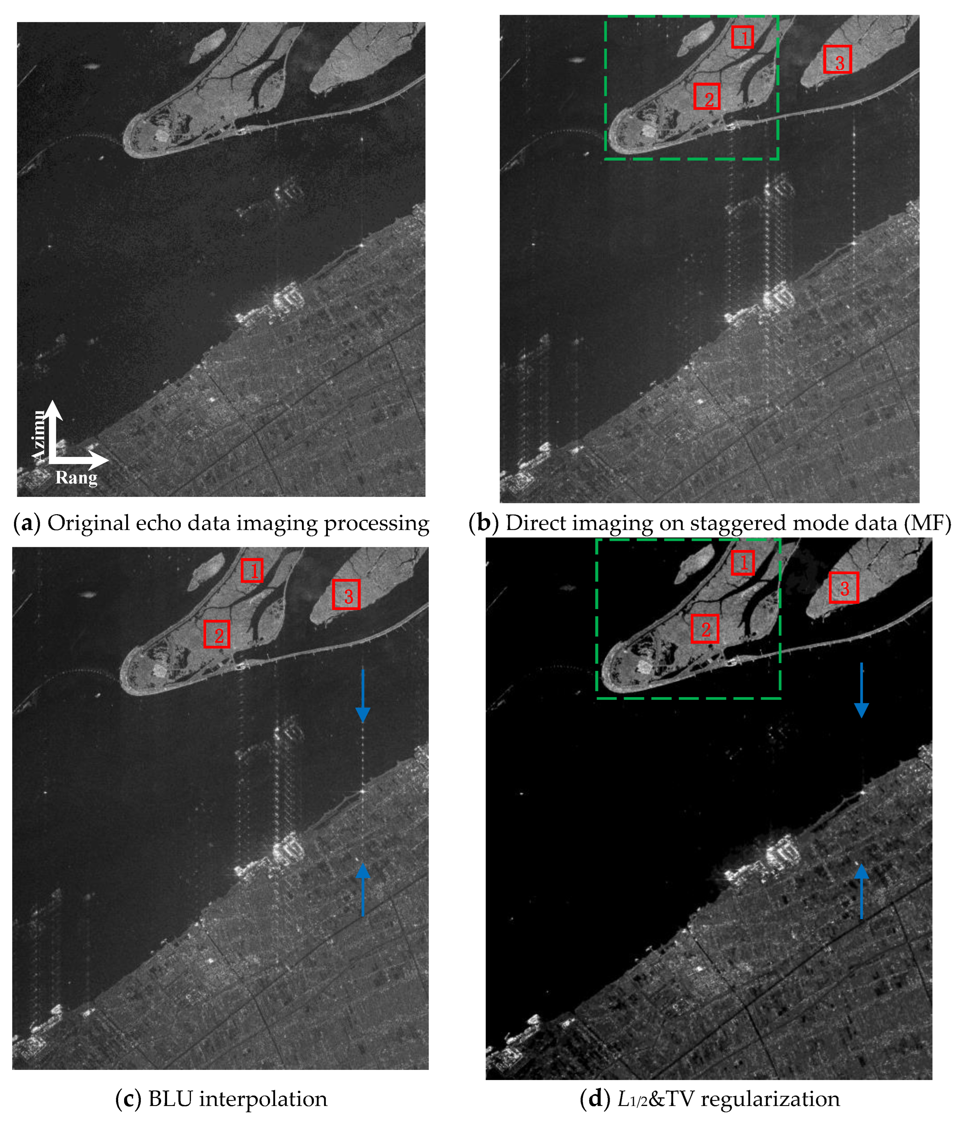
Figure 7 shows the imaging results of different methods in the first sea–land boundary scenario. Figure 7a is the imaging result of the original echo data under the constant PRF condition, with only azimuth ambiguities caused by the nonideal AAP present in the imagery. Figure 7b is the imaging result of the direct MF operation on the missing echo data of the variable PRF mode. It can be seen that there were azimuth ambiguities caused by nonuniform sampling and echo data loss in the image. Figure 7c,d are the imaging results of BLU interpolation and L_1/2&TV regularization under nonuniform sampling conditions, respectively.

Figure 8 compares the imaging results of the BLU interpolation method and the L_1/2&TV regularization-based method, providing the one-dimensional profiles of the strong point target indicated by the blue arrows in Figure 7c,d along the azimuth direction.

In order to verify the effectiveness of the proposed method in improving the accuracy of distributed target reconstruction, three different regions in the first scenario were selected as the research objects, represented by red rectangular frames and named Region 1, Region 2, and Region 3, as shown in Figure 7. The islands where Region 1 and Region 2 are located are represented by green rectangular dashed frames, as shown in Figure 7b,d. The island areas contained in the dashed frames are enlarged and displayed, and the results are shown in Figure 9.

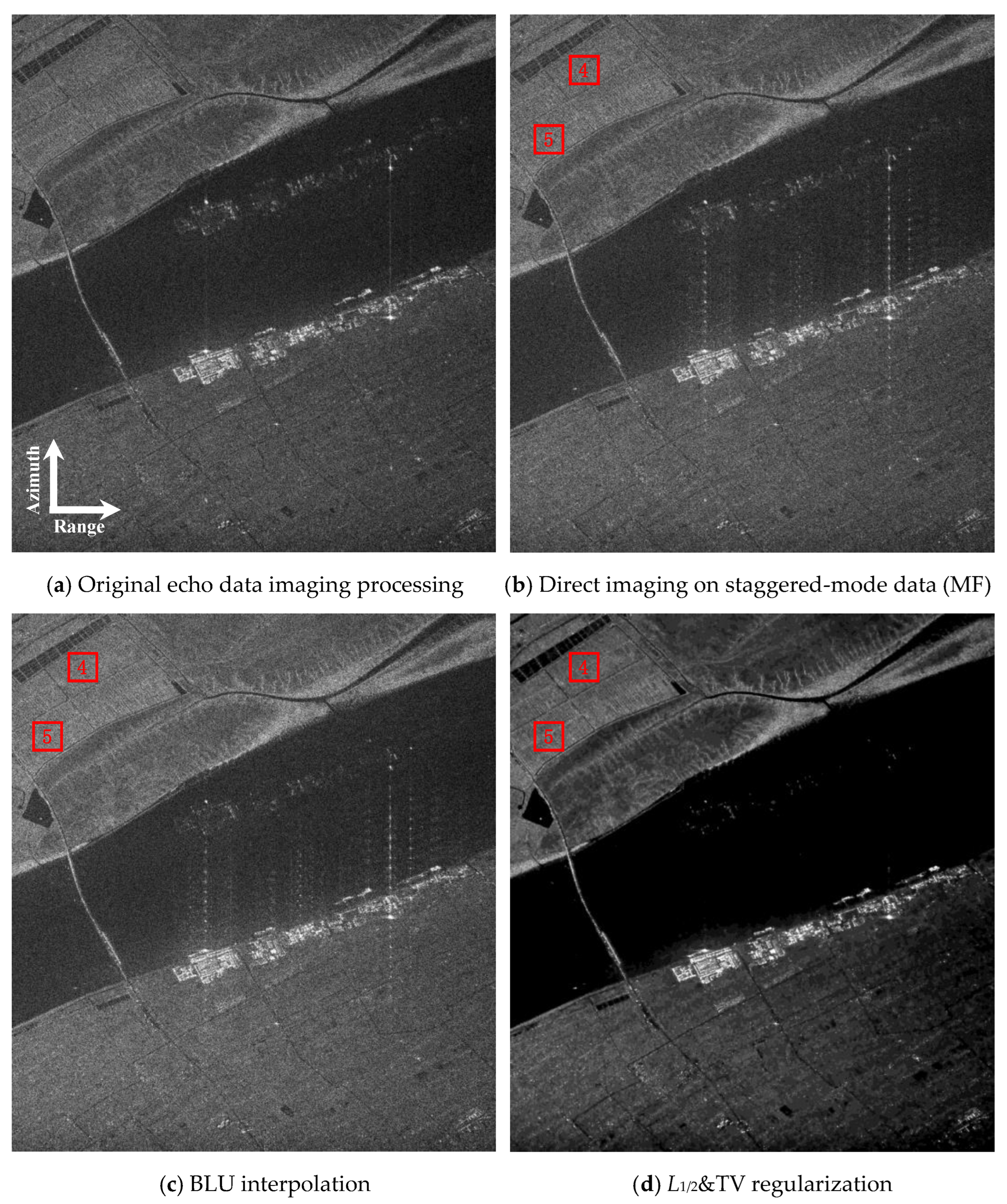
Figure 10 shows the imaging results of different methods in the second sea–land boundary scenario. Similarly, two different regions in the second scenario are selected as the research objects, represented by red rectangular frames and named Region 4 and Region 5.

Next, quantitative calculations were conducted on the continuity of the reconstruction results for Region 1, Region 2, Region 3, Region 4, and Region 5. This paper selects the equivalent number of looks (ENL) as the indicator to measure the coherent speckle suppression effect of SAR images. ENL is an indicator that measures the continuity of a uniform region, and the larger the value of ENL, the better the smoothing effect of the image. The definition of ENL is as follows:

$$ENL=\frac{{{\mu }_I}^2}{{{\sigma }_I}^2},$$

(37)

where ${\mu }_I$ represents the average value of the SAR image intensity and ${{\sigma }_I}^2$ represents the variance of the SAR image intensity. The ENL values of Region 1, Region 2, Region 3, Region 4, and Region 5 were calculated, and the results are shown in

Table 6. ENL values of Region 1 to Region 5 with different imaging methods.

	Region 1	Region 2	Region 3	Region 4	Region 5
BLU	0.9652	0.9677	0.9839	0.9277	0.9303
L1/2&TV	6.4498	6.4546	7.2608	6.4152	6.4265

.

5. Discussion

In this section, we will discuss the experimental results of the previous section in detail. Firstly, the point target simulation experimental results will be discussed. As shown in Figure 2a, the 1-D imaging result of the MF method for the point target located inside the blind areas contains multiple pairs of weak azimuth ambiguities and one pair of strong azimuth ambiguities. Figure 2b presents the imaging result of the BLU interpolation method under the same conditions. Comparing Figure 2a with Figure 2b, it can be found that, under low-oversampling conditions, the results of the BLU interpolation method and the MF method were almost the same, and the azimuth ambiguities could not be suppressed. It can be seen from Figure 3 that, when the azimuth oversampling rate increases, the ISLR values of the three imaging methods all decreased. Moreover, when the oversampling rate is greater than 1.5, that is, in the case of high oversampling, the BLU interpolation method performs better in suppressing azimuth ambiguities caused by nonuniform sampling, but it is not suitable for lower oversampling rates (from 1.1 to 1.5), as shown in Figure 3b. It should be explained that the recovery accuracy of the BLU interpolation algorithm proposed in [22] depends largely on the PRF of the radar system [26]. The accuracy of the interpolation decreases when the PRF is close to the Nyquist frequency and improves as the oversampling rate increases [27,29]. Therefore, the imaging results in Figure 2 and the quantitative calculation results in Table 3 and Figure 3 are consistent with the theoretical analysis. For the point target, the L_1/2&TV regularization actually degenerated into the L_1/2 regularization. Figure 2c presents the imaging result of the L_1/2-regularization-based method when the point target is located inside the blind areas. Combined with the quantitative results in Table 3, it indicates that the proposed method can effectively suppress the azimuth ambiguities caused by nonuniform sampling and echo data loss in the low-oversampled staggered mode, reducing the ISLR value by about 10 dB. In addition, the AASR values in Table 3 also show that the proposed method had a certain suppression effect on the strong azimuth ambiguities caused by the nonideal AAP. By comparing the results of Figure 2 vertically and combining them with Figure 3, we can find that the values of ISLR were different when the point target was located inside the blind areas, at the boundary of the blind areas, and outside the blind areas, respectively. This is because they lose different samples within one PRI variation period. It is obvious that the ambiguity of the point target was the lowest when it was located outside the blind areas. Comparing Figure 3c with Figure 3a, it can be found that the oversampling rate–ISLR relationship curve of the L_1/2-regularization-based method was much lower than that of the MF method under various conditions. Comparing Figure 3c with Figure 3b, although the results of the L_1/2-regularization-based method and the BLU interpolation method were similar under high-oversampling conditions, the former performed significantly better than the latter under low-oversampling conditions. Therefore, the proposed sparse SAR imaging method can effectively solve the problem of azimuth ambiguities caused by nonuniform sampling and echo data loss in the low-oversampled staggered mode.

Secondly, the results of the distributed-targets simulation experiments will be discussed. Figure 4b,c show the imaging results of the MF method and BLU interpolation method for the low-oversampled staggered mode, respectively. It can be seen from Figure 4b that, compared with the point target, for the distributed target, the azimuth ambiguities caused by nonuniform sampling were more dispersed. Although the BLU interpolation method could maintain the scattering characteristics of the distributed target, it could not effectively suppress the azimuth ambiguities under low-oversampling conditions, resulting in almost the same imaging results as the MF method, as shown in Figure 4c. Figure 4d shows the imaging result of the L_1/2&TV regularization-based method proposed in this paper. It can be seen that the proposed method can effectively suppress the azimuth ambiguities caused by nonuniform sampling without recovering the missing echo data and reduce the reconstruction error of the distributed target. Furthermore, the quantitative calculation results in Table 4 indicate that, under the low-oversampling condition (oversampling rate 1.1), the proposed method can significantly reduce the NRMSE value, while the NRMSE value of the BLU interpolation method is not significantly different from that of the MF method. Combined with the imaging results in Figure 4, it can be concluded that the proposed method can reconstruct distributed targets more accurately. This can be explained by the TV norm characteristic [55,56], which can maintain the continuity of the backscattering coefficient of distributed targets. From Figure 5, it can be seen that, in the presence of noise, the proposed L_1/2&TV-regularization-based method can obtain lower NRMSE values than the BLU interpolation method, verifying the accuracy of this method for distributed target reconstruction under low-oversampling conditions. In addition, by comparing Figure 5a,b, it can be seen that, when the distributed target is located at the boundary of the blind areas, the NRMSE values of both methods are lower than those when the target is located inside the blind areas. This indicates that the reconstruction accuracy is related to the number of samples lost within one PRI variation period, and the higher the data loss rate, the lower the reconstruction accuracy. From Figure 6, it can be seen that both the BLU interpolation method and the L_1/2&TV-regularization-based method had reduced NRMSE values as the oversampling rate increased, regardless of whether the distributed target was located inside or at the boundary of the blind areas. This illustrates that the reconstruction accuracy was improved, and the larger the oversampling rate, the better the effect. When the oversampling rate was greater than 1.5, that is, in the case of high oversampling, the NRMSE values of the BLU interpolation method significantly decreased, being even lower than those of the L_1/2&TV-regularization-based method. However, when the oversampling rate was less than 1.2, the reconstruction accuracy of the L_1/2&TV-regularization-based method was superior to that of the BLU interpolation method, further verifying that the proposed method could improve the reconstruction accuracy of distributed targets under low-oversampling conditions. Figure 6 also illustrates the impact of the data loss rate on the accuracy of distributed target reconstruction, which was more evident in low-oversampling cases. The above discussion of the distributed target simulation experimental results prove that the proposed sparse SAR imaging method can improve the reconstruction accuracy of distributed targets and enhance the region-based features of SAR images in the low-oversampled staggered mode.

Thirdly, the results of real data experiments will be discussed. The effectiveness of the proposed method in suppressing azimuth ambiguities is discussed first. Figure 7c presents the imaging result of the BLU interpolation method for the first sea–land boundary scenario. It can be seen that azimuth ambiguities caused by nonuniform sampling still existed in the image, proving its limitations under low-oversampling conditions. Figure 7d is the imaging result of the L_1/2&TV regularization-based method. It can be seen that, due to the azimuth–range decouple operators, the azimuth ambiguities and false targets in the image were effectively suppressed. Figure 8 further illustrates the conclusion. From the comparison results in Figure 8, it can be seen that the BLU interpolation method could not effectively suppress azimuth ambiguities, so it was not suitable for the low-oversampled staggered mode. Compared with the BLU interpolation method, the L_1/2&TV regularization-based method could significantly improve the suppression effect of azimuth ambiguities caused by nonuniform sampling and echo data loss. Next, the effectiveness of the proposed method in improving the accuracy of the distributed target reconstruction is discussed. It can be seen from Figure 9 that there were lots of coherent speckles in the image reconstructed by MF, and the continuity of the island areas could not be satisfied, as shown in Figure 9a. The reconstructed image result using the proposed method was more uniform and continuous, and the coherent speckles and noise in the image were effectively suppressed, as shown in Figure 9b. This proves that the proposed method could maintain the continuity of the backscattering coefficient of distributed targets and improve the reconstruction accuracy of distributed targets for the low-oversampled staggered mode. The numerical calculation results in Table 6 are discussed at the end. As multi-look processing is not performed on real data and the BLU interpolation method actually utilizes matched filtering for imaging processing, the ENL values of the reconstruction result are approximately equal to 1, as shown in the first row of Table 6. In contrast, the L_1/2&TV-regularization-based method can effectively improve the ENL values of the reconstruction result, as shown in the second row of Table 6, further demonstrating that the proposed method can enhance the region-based features of SAR images.

Finally, the comparison of simulation and real data experimental results will be discussed. For the point target simulation, we designed two experiments, as stated above. Both point target simulation experiments verified the effectiveness of the proposed method for suppressing azimuth ambiguities in low-oversampled staggered SAR. However, it should be noted that the point target simulation experiments only considered the L_1/2 regularization term in compound regularization. Similarly, the distributed targets simulation verified the effectiveness of the proposed method for improving the reconstruction accuracy of distributed targets in low-oversampled staggered SAR. But these experiments mainly considered the TV regularization term in compound regularization. Therefore, it is necessary to select appropriate scenarios in real data experiments and verify the effects of L_1/2 regularization and TV regularization simultaneously, as shown in Figure 7 and Figure 10. Since the selected scenarios included both strong point targets and distributed targets, such as island areas, compound regularization can be effectively verified. Comparing Figure 8 with Figure 2, it can be concluded that L_1/2&TV regularization can indeed suppress the azimuth ambiguities caused by nonuniform sampling and echo data loss in the low-oversampled staggered mode. In addition, the ISLR indicators of the azimuth profiles of different imaging methods shown in Figure 8 were quantitatively calculated. The result was that the ISLR value of L_1/2&TV regularization was 12 dB lower than that of BLU interpolation, which was consistent with the calculation results in Table 3. Comparing Table 6 with Table 4, it can be found that two different evaluation indicators (NRMSE and ENL) both demonstrated that L_1/2&TV regularization had more significant advantages in distributed target reconstruction. In summary, the comparison between simulation and real data experiments fully demonstrates the effectiveness of compound regularization in both azimuth ambiguity suppression and accurate reconstruction of distributed targets.

It should be pointed out that, if we want to better suppress the azimuth ambiguities caused by nonideal AAP, the group sparsity property [69] should be considered when constructing the imaging model, and the nonuniform sampling problem should be solved during the group sparse reconstruction process [70]. This is also work we will carry out in the future.

6. Conclusions

This paper proposes a sparse SAR imaging method for the low-oversampled staggered mode via compound regularization. By incorporating the blind area index matrix to represent echo data loss within the sparse imaging model and integrating the L_1/2 regularization term into the sparse reconstruction model, our method effectively mitigates azimuth ambiguities in staggered SAR systems without the need to recover missing data. Furthermore, by applying both the imaging and echo simulation operators specific to staggered SAR systems for azimuth-range decoupling and introducing the TV regularization term into the sparse reconstruction model, our method significantly enhances the reconstruction accuracy of distributed targets. The method’s effectiveness is substantiated through experimental results derived from both simulated data and real spaceborne SAR data.

References

- Amitrano, D.; Di Martino, G.; Guida, R.; Iervolino, P.; Iodice, A.; Papa, M.N.; Riccio, D.; Ruello, G. Earth environmental monitoring using multi-temporal synthetic aperture radar: A critical review of selected applications. Remote Sens. 2021, 13, 604. [Google Scholar] [CrossRef]
- Alessi, M.A.; Chirico, P.G.; Sunder, S.; O’Pry, K.L. Detection and Monitoring of Small-Scale Diamond and Gold Mining Dredges Using Synthetic Aperture Radar on the Kadéï (Sangha) River, Central African Republic. Remote Sens. 2023, 15, 913. [Google Scholar] [CrossRef]
- Braun, A.; Fakhri, F.; Hochschild, V. Refugee camp monitoring and environmental change assessment of Kutupalong, Bangladesh, based on radar imagery of Sentinel-1 and ALOS-2. Remote Sens. 2019, 11, 2047. [Google Scholar] [CrossRef]
- El Hajj, M.; Baghdadi, N.; Zribi, M.; Bazzi, H. Synergic use of Sentinel-1 and Sentinel-2 images for operational soil moisture mapping at high spatial resolution over agricultural areas. Remote Sens. 2017, 9, 1292. [Google Scholar] [CrossRef]
- Mastro, P.; Masiello, G.; Serio, C.; Pepe, A. Change Detection Techniques with Synthetic Aperture Radar Images: Experiments with Random Forests and Sentinel-1 Observations. Remote Sens. 2022, 14, 3323. [Google Scholar] [CrossRef]
- Krieger, G.; Moreira, A. Spaceborne bi-and multistatic SAR: Potential and challenges. IEE Proc. Radar Sonar Navig. 2006, 153, 184–198. [Google Scholar] [CrossRef]
- Currie, A.; Brown, M.A. Wide-swath SAR. IEE Proc. F 1992, 139, 122–135. [Google Scholar] [CrossRef]
- Sikaneta, I.; Gierull, C.H.; Cerutti-Maori, D. Optimum signal processing for multichannel SAR: With application to high-resolution wide-swath imaging. IEEE Trans. Geosci. Remote Sens. 2014, 52, 6095–6109. [Google Scholar] [CrossRef]
- Krieger, G.; Gebert, N.; Moreira, A. Unambiguous SAR signal reconstruction from nonuniform displaced phase center sampling. IEEE Geosci. Remote Sens. Lett. 2004, 1, 260–264. [Google Scholar] [CrossRef]
- Zhang, S.X.; Xing, M.D.; Xia, X.G.; Zhang, L.; Guo, R.; Liao, Y.; Bao, Z. Multichannel HRWS SAR imaging based on range-variant channel calibration and multi-Doppler-direction restriction ambiguity suppression. IEEE Trans. Geosci. Remote Sens. 2014, 52, 4306–4327. [Google Scholar] [CrossRef]
- Baumgartner, S.V.; Krieger, G. Simultaneous high-resolution wide-swath SAR imaging and ground moving target indication: Processing approaches and system concepts. IEEE J. Sel. Top. Appl. Earth Obs. Remote Sens. 2015, 8, 5015–5029. [Google Scholar] [CrossRef]
- Krieger, G. MIMO-SAR: Opportunities and pitfalls. IEEE Trans. Geosci. Remote Sens. 2014, 52, 2628–2645. [Google Scholar] [CrossRef]
- Kim, J.H.; Younis, M.; Moreira, A.; Wiesbeck, W. Spaceborne MIMO synthetic aperture radar for multimodal operation. IEEE Trans. Geosci. Remote Sens. 2015, 53, 2453–2466. [Google Scholar] [CrossRef]
- Kim, S.; Yu, J.; Jeon, S.Y.; Dewantari, A.; Ka, M.H. Signal processing for a multiple-input, multiple-output (MIMO) video synthetic aperture radar (SAR) with beat frequency division frequency-modulated continuous wave (FMCW). Remote Sens. 2017, 9, 491. [Google Scholar] [CrossRef]
- Younis, M.; Fischer, C.; Wiesbeck, W. Digital beamforming in SAR systems. IEEE Trans. Geosci. Remote Sens. 2003, 41, 1735–1739. [Google Scholar] [CrossRef]
- Reigber, A.; Schreiber, E.; Trappschuh, K.; Pasch, S.; Müller, G.; Kirchner, D.; Geßwein, D.; Schewe, S.; Nottensteiner, A.; Limbach, M.; et al. The High-Resolution Digital-Beamforming Airborne SAR System DBFSAR. Remote Sens. 2020, 12, 1710. [Google Scholar] [CrossRef]
- Gebert, N.; Krieger, G. Ultra-wide swath SAR imaging with continuous PRF variation. In Proceedings of the EUSAR 2010: 8th European Conference on Synthetic Aperture Radar, Aachen, Germany, 7–10 June 2010; pp. 1–4. [Google Scholar]
- Villano, M.; Krieger, G.; Moreira, A. Staggered-SAR for high-resolution wide-swath imaging. In Proceedings of the IET International Conference on Radar Systems, Glasgow, UK, 22–25 October 2012; pp. 1–6. [Google Scholar]
- Luo, X.L.; Wang, R.; Xu, W.; Deng, Y.K.; Guo, L. Modification of multichannel reconstruction algorithm on the SAR with linear variation of PRI. IEEE J. Sel. Top. Appl. Earth Obs. Remote Sens. 2014, 7, 3050–3059. [Google Scholar] [CrossRef]
- Villano, M.; Krieger, G. Staggered SAR: From concept to experiments with real data. In Proceedings of the EUSAR 2014: 10th European Conference on Synthetic Aperture Radar, Berlin, Germany, 3–5 June 2014; pp. 1–4. [Google Scholar]
- Villano, M.; Krieger, G.; Moreira, A. A novel processing strategy for staggered SAR. IEEE Geosci. Remote Sens. Lett. 2014, 11, 1891–1895. [Google Scholar] [CrossRef]
- Villano, M.; Krieger, G.; Moreira, A. Staggered SAR: High-resolution wide-swath imaging by continuous PRI variation. IEEE Trans. Geosci. Remote Sens. 2014, 52, 4462–4479. [Google Scholar] [CrossRef]
- Villano, M.; Krieger, G.; Moreira, A. Onboard processing for data volume reduction in high-resolution wide-swath SAR. IEEE Geosci. Remote Sens. Lett. 2016, 13, 1173–1177. [Google Scholar] [CrossRef]
- Moreira, A.; Krieger, G.; Hajnsek, I.; Papathanassiou, K.; Younis, M.; Lopez-dekker, P.; Huber, S.; Villano, M.; Pardini, M. Tandem-L: A highly innovative bistatic SAR mission for global observation of dynamic processes on the Earth’s surface. IEEE Geosci. Remote Sens. Mag. 2015, 3, 8–23. [Google Scholar] [CrossRef]
- Huber, S.; de Almeida, F.Q.; Villano, M.; Younis, M.; Krieger, G.; Moreira, A. Tandem-L: A technical perspective on future spaceborne SAR sensors for Earth observation. IEEE Trans. Geosci. Remote Sens. 2018, 56, 4792–4807. [Google Scholar] [CrossRef]
- Liao, X.X.; Jin, C.L.; Liu, Z. Compressed Sensing Imaging for Staggered SAR with Low Oversampling Ratio. In Proceedings of the EUSAR 2021—13th European Conference on Synthetic Aperture Radar, Online, 29 March–1 April 2021; pp. 1–4. [Google Scholar]
- Pinheiro, M.; Prats-Iraola, P.; Rodriguez-Cassola, M.; Villano, M. Analysis of low-oversampled Staggered SAR data. IEEE J. Sel. Top. Appl. Earth Obs. Remote Sens. 2020, 13, 241–255. [Google Scholar] [CrossRef]
- Zhou, Z.X.; Deng, Y.K.; Wang, W.; Jia, X.L.; Wang, R. Linear Bayesian approaches for low-oversampled stepwise staggered SAR data. IEEE Trans. Geosci. Remote Sens. 2021, 60, 1–23. [Google Scholar] [CrossRef]
- Wang, X.Y.; Wang, R.; Deng, Y.K.; Wang, W.; Li, N. SAR signal recovery and reconstruction in staggered mode with low oversampling factors. IEEE Geosci. Remote Sens. Lett. 2018, 15, 704–708. [Google Scholar] [CrossRef]
- Yardibi, T.; Li, J.; Stoica, P.; Xue, M.; Baggeroer, A.B. Source localization and sensing: A nonparametric iterative adaptive approach based on weighted least squares. IEEE Trans. Aerosp. Electron. Syst. 2010, 46, 425–443. [Google Scholar] [CrossRef]
- Pinheiro, M.; Prats-Iraola, P.; Rodriguez-Cassola, M.; Villano, M. Combining spectral estimation and BLU interpolation for the reconstruction of low-oversampled Staggered SAR data. In Proceedings of the EUSAR 2018: 12th European Conference on Synthetic Aperture Radar, Aachen, Germany, 4–7 June 2018; pp. 1–6. [Google Scholar]
- Donoho, D.L. Compressed sensing. IEEE Trans. Inf. Theory 2006, 52, 1289–1306. [Google Scholar] [CrossRef]
- Candès, E.J.; Wakin, M.B. An introduction to compressive sampling. IEEE Signal Process. Mag. 2008, 25, 21–30. [Google Scholar] [CrossRef]
- Herman, M.A.; Strohmer, T. High-resolution radar via compressed sensing. IEEE Trans. Signal Process. 2009, 57, 2275–2284. [Google Scholar] [CrossRef]
- Xu, J.; Pi, Y.; Cao, Z. Bayesian compressive sensing in synthetic aperture radar imaging. IET Radar Sonar Navig. 2012, 6, 2–8. [Google Scholar] [CrossRef]
- Candès, E.J.; Romberg, J.K.; Tao, T. Stable signal recovery from incomplete and inaccurate measurements. Commun. Pure Appl. Math. 2006, 59, 1207–1223. [Google Scholar] [CrossRef]
- Nyquist, H. Certain topics in telegraph transmission theory. Trans. Am. Inst. Electr. Eng. 1928, 47, 617–644. [Google Scholar] [CrossRef]
- Shannon, C.E. Communication in the presence of noise. Proc. Inst. Radio Eng. 1949, 37, 10–21. [Google Scholar] [CrossRef]
- Çetin, M.; Karl, W.C. Feature-enhanced synthetic aperture radar image formation based on nonquadratic regularization. IEEE Trans. Image Process. 2001, 10, 623–631. [Google Scholar] [CrossRef] [PubMed]
- Patel, V.M.; Easley, G.R.; Healy, D.M., Jr.; Chellappa, R. Compressed synthetic aperture radar. IEEE J. Sel. Topics Signal Process. 2010, 4, 244–254. [Google Scholar] [CrossRef]
- Stojanovic, I.; Çetin, M.; Karl, W.C. Compressed sensing of monostatic and multistatic SAR. IEEE Geosci. Remote Sens. Lett. 2013, 10, 1444–1448. [Google Scholar] [CrossRef]
- Zhang, B.C.; Hong, W.; Wu, Y.R. Sparse microwave imaging: Principles and applications. Sci. China Inf. Sci. 2012, 55, 1722–1754. [Google Scholar] [CrossRef]
- Çetin, M.; Stojanović, I.; Önhon, N.Ö.; Varshney, K.; Samadi, S.; Karl, W.C.; Willsky, A.S. Sparsity-driven synthetic aperture radar imaging: Reconstruction, autofocusing, moving targets, and compressed sensing. IEEE Signal Process. Mag. 2014, 31, 27–40. [Google Scholar] [CrossRef]
- Fang, J.; Xu, Z.B.; Zhang, B.C.; Hong, W.; Wu, Y.R. Fast compressed sensing SAR imaging based on approximated observation. IEEE J. Sel. Top. Appl. Earth Obs. Remote Sens. 2013, 7, 352–363. [Google Scholar] [CrossRef]
- Zhang, B.C.; Zhang, Z.; Jiang, C.L.; Zhao, Y.; Hong, W.; Wu, Y.R. System design and first airborne experiment of sparse microwave imaging radar: Initial results. Sci. China Inf. Sci. 2015, 6, 1–10. [Google Scholar] [CrossRef]
- Xu, Z.L.; Wei, Z.H.; Wu, C.Y.; Zhang, B.C. Multichannel sliding spotlight SAR imaging based on sparse signal processing. In Proceedings of the IGARSS 2018—2018 IEEE International Geoscience and Remote Sensing Symposium, Valencia, Spain, 22–27 July 2018; pp. 3703–3706. [Google Scholar]
- Bi, H.; Zhang, B.C.; Zhu, X.X.; Jiang, C.L.; Hong, W. Extended chirp scaling-baseband azimuth scaling-based azimuth-range decouple L1 regularization for TOPS SAR imaging via CAMP. IEEE Trans. Geosci. Remote Sens. 2017, 55, 3748–3763. [Google Scholar] [CrossRef]
- Yang, X.Y.; Li, G.; Sun, J.P.; Liu, Y.; Xia, X.G. High-resolution and wide-swath SAR imaging via Poisson disk sampling and iterative shrinkage thresholding. IEEE Trans. Geosci. Remote Sens. 2019, 57, 4692–4704. [Google Scholar] [CrossRef]
- Pu, W.; Wu, J.J. OSRanP: A novel way for radar imaging utilizing joint sparsity and low-rankness. IEEE Trans. Comput. Imaging 2020, 6, 868–882. [Google Scholar] [CrossRef]
- Shen, F.F.; Zhao, G.H.; Liu, Z.C.; Shi, G.M.; Lin, J. SAR imaging with structural sparse representation. IEEE J. Sel. Top. Appl. Earth Obs. Remote Sens. 2014, 8, 3902–3910. [Google Scholar] [CrossRef]
- Osher, S.; Ruan, F.; Xiong, J.; Yao, Y.; Yin, W. Sparse recovery via differential inclusions. Appl. Comput. Harmon. Anal. 2016, 41, 436–469. [Google Scholar] [CrossRef]
- Xu, Z.B.; Chang, X.Y.; Xu, F.M.; Zhang, H. L1/2 regularization: A thresholding representation theory and a fast solver. IEEE Trans. Neural Netw. Learn. Syst. 2012, 23, 1013–1027. [Google Scholar] [PubMed]
- Xu, Z.B.; Zhang, H.; Wang, Y.; Chang, X.Y.; Liang, Y. L1/2 regularization. Sci. China Inf. Sci. 2010, 53, 1159–1169. [Google Scholar] [CrossRef]
- Xu, Z.Q.; Liu, M.Q.; Zhou, G.R.; Wei, Z.H.; Zhang, B.C.; Wu, Y.R. An accurate sparse SAR imaging method for enhancing region-based features via nonconvex and TV regularization. IEEE J. Sel. Top. Appl. Earth Obs. Remote Sens. 2020, 14, 350–363. [Google Scholar] [CrossRef]
- Chambolle, A. An algorithm for total variation minimization and applications. J. Math. Imaging Vis. 2004, 20, 89–97. [Google Scholar]
- Chambolle, A. Total variation minimization and a class of binary MRF models. In Proceedings of the International Workshop on Energy Minimization Methods in Computer Vision and Pattern Recognition, St. Augustine, FL, USA, 9–11 November 2015; Springer: Berlin/Heidelberg, Germany, 2005; pp. 136–152. [Google Scholar]
- Wang, S.; Xu, H.P.; Zhang, J.W. A SAR imaging method based on Lp and TV composite norm regularization. In Proceedings of the IGARSS 2020—2020 IEEE International Geoscience and Remote Sensing Symposium, Waikoloa, HI, USA, 26 September–2 October 2020; pp. 1149–1152. [Google Scholar]
- Cai, J.; Meng, Z.; Ho, C.M. Residual channel attention generative adversarial network for image super-resolution and noise reduction. In Proceedings of the IEEE/CVF Conference on Computer Vision and Pattern Recognition Workshops, Seattle, WA, USA, 14–19 June 2020; pp. 454–455. [Google Scholar]
- Khan, M.; Gueaieb, W.; El Saddik, A.; Kwon, S. MSER: Multimodal speech emotion recognition using cross-attention with deep fusion. Expert Syst. Appl. 2024, 245, 122946. [Google Scholar] [CrossRef]
- Afonso, M.V.; Bioucas-Dias, J.M.; Figueiredo, M.A.T. An augmented Lagrangian approach to the constrained optimization formulation of imaging inverse problems. IEEE Trans. Image Process. 2010, 20, 681–695. [Google Scholar] [CrossRef] [PubMed]
- Jiang, C.L.; Zhang, B.C.; Fang, J.; Zhang, Z.; Hong, W.; Wu, Y.R.; Xu, Z.B. Efficient ℓq regularisation algorithm with range–azimuth decoupled for SAR imaging. Electron. Lett. 2014, 50, 204–205. [Google Scholar] [CrossRef]
- Raney, R.K.; Runge, H.; Bamler, R.; Cumming, I.G.; Wong, F.H. Precision SAR processing using chirp scaling. IEEE Trans. Geosci. Remote Sens. 1994, 32, 786–799. [Google Scholar] [CrossRef]
- Daubechies, I.; Defrise, M.; De Mol, C. An iterative thresholding algorithm for linear inverse problems with a sparsity constraint. Commun. Pure Appl. Math. J. Issued Courant Inst. Math. Sci. 2004, 57, 1413–1457. [Google Scholar] [CrossRef]
- Bioucas-Dias, J.M.; Figueiredo, M.A.T. Two-step algorithms for linear inverse problems with non-quadratic regularization. In Proceedings of the 2007 IEEE International Conference on Image Processing, Antonio, TX, USA, 16 September–19 October 2007; Volume 1, pp. I-105–I-108. [Google Scholar]
- Beck, A.; Teboulle, M. A fast iterative shrinkage-thresholding algorithm for linear inverse problems. SIAM J. Imaging Sci. 2009, 2, 183–202. [Google Scholar] [CrossRef]
- Anitori, L.; Maleki, A.; Otten, M.; Baraniuk, R.G.; Hoogeboom, P. Design and analysis of compressed sensing radar detectors. IEEE Trans. Signal Process. 2012, 61, 813–827. [Google Scholar] [CrossRef]
- Maleki, A.; Anitori, L.; Yang, Z.; Baraniuk, R.G. Asymptotic analysis of complex LASSO via complex approximate message passing (CAMP). IEEE Trans. Inf. Theory 2013, 59, 4290–4308. [Google Scholar] [CrossRef]
- Liu, M.Q.; Zhang, B.C.; Xu, Z.Q.; Zhang, Y.; Zhong, L.H.; Wu, Y.R. Ambiguities Suppression for Azimuth Multichannel SAR Based on L2, q Regularization with Application to Gaofen-3 Ultra-Fine Stripmap Mode. IEEE J. Sel. Top. Appl. Earth Obs. Remote Sens. 2020, 14, 1532–1544. [Google Scholar] [CrossRef]
- Baron, D.; Duarte, M.F.; Wakin, M.B.; Sarvotham, S. Distributed Compressive Sensing. arXiv 2009, arXiv:0901.3403. [Google Scholar]
- Zhang, B.C.; Jiang, C.L.; Zhang, Z. Azimuth ambiguity suppression for SAR imaging based on group sparse reconstruction. In Proceedings of the 2nd International Workshop on Compressed Sensing Applied to Radar, Bonn, Germany, 17–19 September 2013; pp. 17–19. [Google Scholar]
Figure 1.
PRI sequence values and blind areas’ position in the simulation experiments. (a) The fast-changing PRI sequence values correspond to the parameters in Table 2, where the x-axis ‘m’ is the sequence number; (b) The blind areas’ position of the fast-changing PRI sequence.
Figure 2.
The 1-D imaging results with different methods. (a–c) are the imaging results of the point target located inside the blind areas, respectively (slant range = 956 km); (d–f) are the imaging results of the point target located at the boundary of the blind areas, respectively (slant range = 982 km); (g–i) are the imaging results of the point target located outside the blind areas, respectively (slant range = 994 km).
Figure 3.
The oversampling rate–ISLR relationship curves. (a) Using the MF method; (b) using the BLU interpolation method; and (c) using the L1/2&TV-regularization-based method.
Figure 4.
The imaging results of a one-dimensional distributed target with different methods, where the distributed target is located inside the blind areas (slant range = 956 km). (a) The ideal case; (b) Using the MF method; (c) Using the BLU interpolation method; and (d) Using the L1/2&TV-regularization-based method.
Figure 5.
Comparison curves of the NRMSE reconstructed by BLU interpolation and L1/2&TV regularization under different SNRs. (a) Inside the blind areas (slant range = 956 km); (b) At the boundary of the blind areas (slant range = 982 km).
Figure 6.
The oversampling rate–NRMSE relationship curves. (a) Using the BLU interpolation method; (b) Using the L1/2&TV-regularization-based method.
Figure 7.
The imaging results of different methods in the first actual scenario. (a) Original echo data imaging processing under constant PRF condition; (b) Direct imaging on staggered-mode SAR data (MF); (c) Using the BLU interpolation method; (d) Using the L1/2&TV-regularization-based method.
Figure 8.
The azimuth profiles of the strong point target indicated by the blue arrows in Figure 7.
Figure 9.
The reconstruction results of the island areas represented by the green rectangular dashed frames in Figure 7. (a) MF; (b) L1/2&TV regularization.
Figure 10.
The imaging results of different methods in the second scenario. (a) Original echo data imaging processing under constant PRF condition; (b) Direct imaging on staggered mode SAR data (MF); (c) Using the BLU interpolation method; (d) Using the L1/2&TV regularization-based method.