
Estimation of Small-Stream Water Surface Elevation Using UAV Photogrammetry and Deep Learning
by
 , , , and
Radosław Szostak
1,*,
Marcin Pietroń
2,
Przemysław Wachniew
1,
Mirosław Zimnoch
1 and
and
Paweł Ćwiąkała
3 1
Faculty of Physics and Applied Computer Science, AGH University of Kraków, 19 Reymonta St., 30-059 Krakow, Poland
2
Faculty of Computer Science, Electronics and Telecommunications, AGH University of Kraków, 30 Mickiewicza Av., 30-059 Krakow, Poland
3
Faculty of Geo-Data Science, Geodesy, and Environmental Engineering, AGH University of Kraków, 30 Mickiewicza Av., 30-059 Krakow, Poland
*
Author to whom correspondence should be addressed.
Remote Sens. 2024, 16(8), 1458; https://doi.org/10.3390/rs16081458
Submission received: 28 January 2024
/
Revised: 14 April 2024
/
Accepted: 17 April 2024
/
Published: 20 April 2024
(This article belongs to the Special Issue Computational Intelligence for Remote Sensing Image Analysis and Applications)
Abstract
:Unmanned aerial vehicle (UAV) photogrammetry allows the generation of orthophoto and digital surface model (DSM) rasters of terrain. However, DSMs of water bodies mapped using this technique often reveal distortions in the water surface, thereby impeding the accurate sampling of water surface elevation (WSE) from DSMs. This study investigates the capability of deep neural networks to accommodate the aforementioned perturbations and effectively estimate WSE from photogrammetric rasters. Convolutional neural networks (CNNs) were employed for this purpose. Two regression approaches utilizing CNNs were explored: direct regression employing an encoder and a solution based on prediction of the weight mask by an autoencoder architecture, subsequently used to sample values from the photogrammetric DSM. The dataset employed in this study comprises data collected from five case studies of small lowland streams in Poland and Denmark, consisting of 322 DSM and orthophoto raster samples. A grid search was employed to identify the optimal combination of encoder, mask generation architecture, and batch size among multiple candidates. Solutions were evaluated using two cross-validation methods: stratified k-fold cross-validation, where validation subsets maintained the same proportion of samples from all case studies, and leave-one-case-out cross-validation, where the validation dataset originates entirely from a single case study, and the training set consists of samples from other case studies. Depending on the case study and the level of validation strictness, the proposed solution achieved a root mean square error (RMSE) ranging between 2 cm and 16 cm. The proposed method outperforms methods based on the straightforward sampling of photogrammetric DSM, achieving, on average, an 84% lower RMSE for stratified cross-validation and a 62% lower RMSE for all-in-case-out cross-validation. By utilizing data from other research, the proposed solution was compared on the same case study with other UAV-based methods. For that benchmark case study, the proposed solution achieved an RMSE score of 5.9 cm for all-in-case-out cross-validation and 3.5 cm for stratified cross-validation, which is close to the result achieved by the radar-based method (RMSE of 3 cm), which is considered the most accurate method available. The proposed solution is characterized by a high degree of explainability and generalization.
1. Introduction
The management of water resources constitutes one of central issues of the sustainable development for the environment and human health. The responsible use of water resources relies on understanding the complex and interrelated processes that affect the quantity and quality of water available for human needs, economic activities, and ecosystems. Global demand for freshwater has continued to increase at a rate of 1% per year since 1980, driven by population growth and socioeconomic changes. Simultaneously, the increase in evaporation caused by rising temperatures has led to a decrease in streamflow volumes in many areas of the world, which already suffer from water scarcity problems [1,2]. Achieving socioeconomic and environmental sustainability under such challenging conditions will require the application of innovative technologies, capable of measuring hydrological characteristics at a range of spatial and temporal scales [3].
Traditional surface water management practices are primarily based on data collected from networks of in situ hydrometric gauges. However, they offer limited insights, suitable predominantly for scenarios where the flow is constrained by a well-defined channel boundary. Point measurements do not provide sufficient spatial resolution to fully characterize complex spatial intricacies of surface water extent, like floodplain flows and riparian wetlands [4]. Moreover, access to river banks is often difficult or even dangerous. Spatially distributed water surface elevation (WSE) is used for the validation and calibration of hydrologic, hydraulic, or hydrodynamic models to make hydrological forecasts, including predicting dangerous events such as floods and droughts [5,6,7,8,9,10]. Another important aspect is the decline in existing measurement networks observed in many regions the world [11,12]. The problem is particularly evident in non-industrialized areas, where the density of hydrological measurement networks is many times lower than in developed areas [4].
Remote sensing methods are considered a solution to cover data gaps specific to point measurement networks [13]. For decades, a leading example of remote sensing has been measurements made from satellites [14,15]. Radar altimetry techniques, as demonstrated by measurements from the Envisat [16] and Sentinel 3 [17] satellites, were employed to measure the WSE of rivers. However, due to spatial resolution limitations, these measurements are primarily applicable to monitoring large rivers with a width exceeding 100 m. The root mean square error (RMSE) scores of these solutions range widely, from 2.9 cm to 69 cm, depending on the width of the examined river [18,19]. In addition to the general purpose satellite missions mentioned above, more recently a new satellite mission called Surface Water and Ocean Topography (SWOT) has been launched. This mission is specifically designed for altimetry measurements of both oceanic and terrestrial water bodies. It is anticipated that it will enable measurements of rivers wider than 100 m with a WSE measurement accuracy of 10 cm [20,21].
Small surface streams of the first and second order (according to Strahler’s classification [22]) constitute 70–80% of the length of all rivers in the world and play a significant role in hydrological systems and provide an ecosystem for living organisms [23]. Satellite measurements with limited spatial resolution lack the capability to offer useful WSE measurements for small streams. In this regard, measurement techniques based on unmanned aerial vehicles (UAVs) are promising in many key aspects, as they provide observations in high spatial and temporal resolution, their deployment is simple and fast, and can be used in inaccessible locations [24].
To date, remote sensing methods for measuring WSE in small streams mainly rely on the use of UAVs with various types of sensors attached. A clear comparison in this matter was made by Bandini et al. [25] where UAV based methods using radar, lidar and photogrammetry were compared on the same case study. As a result, the method using radar with an RMSE of 3 cm proved to be far superior to methods based on photogrammetry and lidar with an RMSEs of 16 cm and 22 cm, respectively. In addition to its high accuracy, the advantage of a radar-based solution is the short acquisition and processing time. Nonetheless, this approach necessitates non-standard UAV instrumentation and the requisite knowledge for its configuration. A radar-based solution requires the use of a precise differential localization system such as real-time kinematic (RTK) or post-processing kinematic (PPK) requiring a reference base station operating nearby.
In certain scenarios, photogrammetry presents itself as a preferable alternative to radar. Photogrammetry utilizes a camera as its sensor, a component readily available on the majority of commercially accessible UAVs. Notably, unlike radar, photogrammetry does not necessitate the use of a precise differential positioning system. Georeferencing in photogrammetry can be achieved through pre-established ground control points, eliminating the ongoing need for a base station setup. Consequently, the absence of the necessity to construct and configure a radar sensor and establish an RTK reference station renders photogrammetry particularly advantageous in scenarios requiring cyclic measurements of the spatial distribution of the WSE. Once ground control points are established, they can be utilized repeatedly, enhancing the efficiency and effectiveness of the monitoring process.
Photogrammetric structure-from-motion (SFM) algorithms are able to generate orthophotos and digital surface models (DSMs) of terrain from multiple aerial photographs. Photogrammetric DSMs are precise in determining the elevation of solid surfaces to within a few centimeters [26,27], but water surfaces are usually falsely stated. This is related to the fact that the general principle of SFM algorithms is based on the automatic search for distinguishable and static terrain points that appear in several images showing these points from different perspectives. The surface of water lacks such points as it is uniform, transparent, and in motion. The transparency of the water makes the surface level of the stream depicted on the photogrammetric DSM lower than in reality. The stream bottom is represented by photogrammetric DSMs for clear and shallow streams [28]. Photogrammetric DSMs for opaque water bodies are affected by artifacts brought on by lack of distinguishable key points [29]. The above factors make the measurement of WSE by direct DSM sampling yield results with high uncertainty. Some studies report that it is possible to read the WSE from a photogrammetric DSM near streambank where the stream is shallow and there are no undesirable effects associated with light penetration below the water surface [29,30,31]. However, this method gives satisfactory results only for unvegetated and smoothly sloping streambanks where the boundary line between the water and the land is easy to define [25]. For this reason, this method is not suitable for many streams that do not meet these conditions.
The exponentially growing interest in [32] and the promising results of machine learning algorithms in various fields offer prospects for the application of this technology for estimation of stream WSE. The topic remains insufficiently explored. There are only a few loosely related studies on the subject. Convolutional neural networks (CNNs) were used to estimate water surface elevation in laboratory conditions using high-speed camera recordings of water surface waves [33]. In another study, several machine learning approaches were tested to extract flood water depth based on synthetic aperture radar and DSM data [34]. In the context of using photogrammetric DSM to estimate river water levels, artificial intelligence appears to be a promising tool. Thanks to its flexibility, it can potentially take into account a number of the adverse factors mentioned above and make a more accurate estimate of the WSE compared to direct DSM sampling.
The objective of this study is to assess the capability of CNNs in handling the disturbances in water areas present in photogrammetric DSMs of small streams, with the aim of accurately estimating the WSE.
2. Materials and Methods
2.1. Case Study Site
Photogrammetric data and WSE observations were obtained for Kocinka—a small lowland stream (length 40 km, catchment area 260 km2) located in the Odra River basin in southern Poland. Data were collected on two stream stretches with similar hydromorphological characteristics and different water transparency:
- An approximately 700 m stretch of the Kocinka stream located near the village of Grodzisko (50.8744°N, 18.9711°E). This stretch has a water surface width of about 2 m. There are no trees in close proximity to the stream. The streambed is made up of dark silt and the water is opaque. The banks and the streambed are overgrown with rushes that protrude above the water surface. The banks are steeply sloping at angles of about 50° to 90° relative to the water surface. There are marshes nearby, with stream water flowing into them in places. Data from this stretch were collected on the following days:
- ○
- 19 December 2020. Total cloud cover was present during the measurements. Due to the winter season, the foliage was reduced. Samples obtained from this survey are labeled with the identifier “GRO20”.
- ○
- 13 July 2021. There was no cloud cover during the measurements. The rushes were high and the water surface was densely covered with Lemna plants. Samples obtained from this survey are labeled with the identifier “GRO21”.
- An approximately 700 m stretch of the Kocinka stream located near the village of Rybna (50.9376°N, 19.1143°E). This stretch has a water surface width of about 3 m and is overhung by sparse deciduous trees. There is a pale, sandy streambed that is visible through the clear water. There are no rushes that emerge from the streambed. The banks slope at angles of about 20° to 90° relative to the water surface. Data from this stretch were collected on the following days:
- ○
- 19 December 2020. Total cloud cover was present during the measurements. Due to the winter season, the trees were devoid of leaves and the grasses were reduced. Samples obtained from this survey are labeled with the identifier “RYB20”.
- ○
- 13 July 2021. There was no cloud cover during the measurements. The streambank grasses were high. With good lighting and exceptionally clear water, the streambed was clearly visible through the water. The samples obtained from this survey are labeled with the identifier “RYB21”.
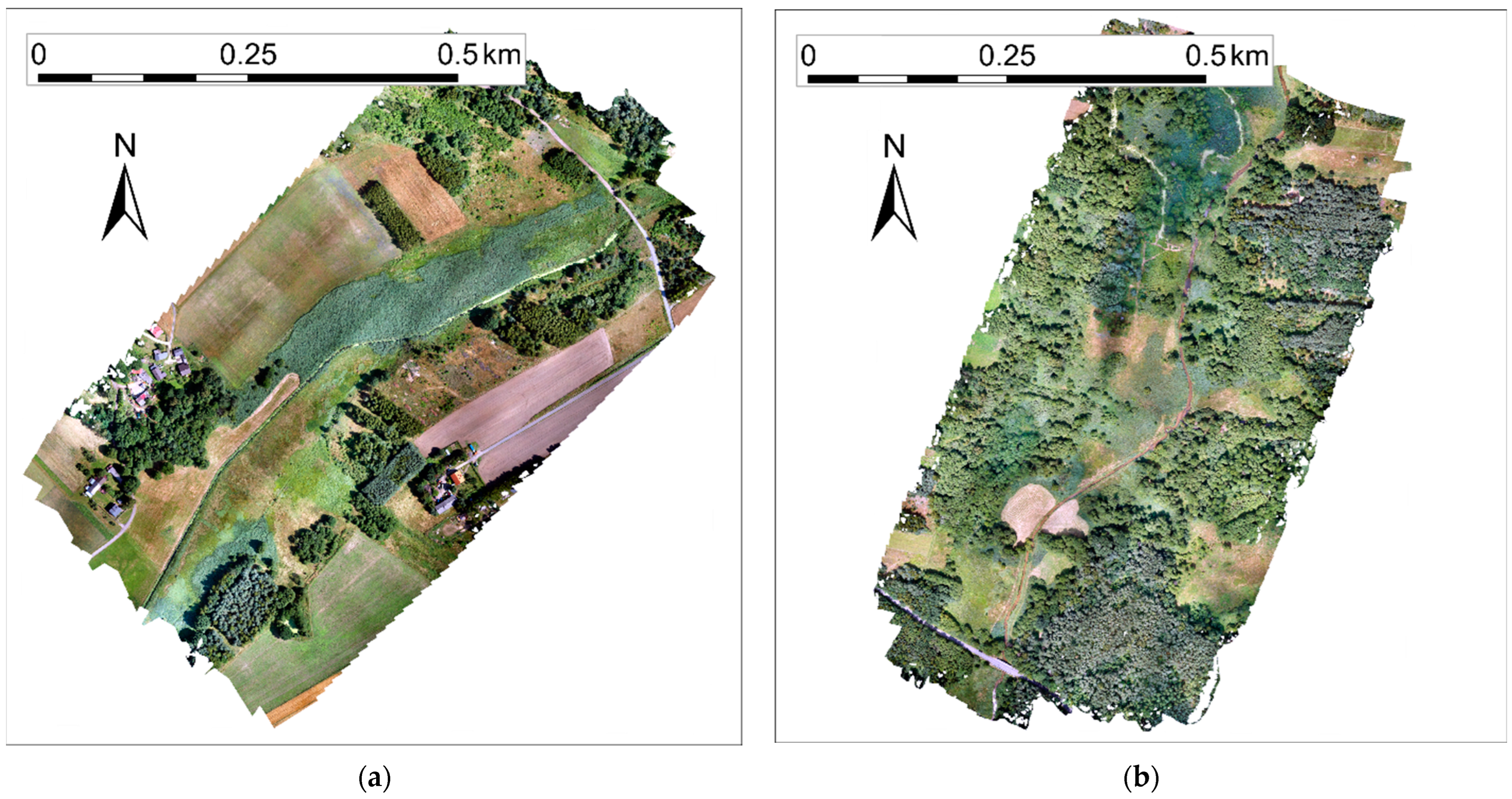
The orthophotos of the Grodzisko and Rybna case studies are shown in Figure 1. The photo of part of the Rybna case study is shown in Figure 2.
Furthermore, the data set was supplemented with data from surveys conducted by Bandini et al. [35] over approximately 2.3 km stretch of the stream Åmose Å (Denmark) on 21 November 2018. The stream is channelized and well maintained. The banks are overgrown with low grass and the neighboring few trees are devoid of leaves due to winter. Further details about this case study can be found in a related study, where current state-of-the-art methods to measure stream WSE with UAVs using radar, lidar, and photogrammetry were tested [25]. The supplemented data is therefore a comparative benchmark to evaluate the proposed method against existing ones. The samples obtained from this survey are labeled in our data set with the identifier “AMO18”.
2.2. Field Surveys
During the survey campaigns, photogrammetric measurements were conducted over the stream area. Aerial photos were taken from a DJI S900 (DJI, Shenzhen, China) UAV using a Sony ILCE a6000 (Sony, Bangkok, Thailand) camera with a Voigtlander SUPER WIDE HELIAR VM 15 mm f/4.5 (Voigtlander, Nagano, Japan) lens. The flight altitude was approximately 77 m above ground level, resulting in a 20 mm terrain pixel. The front overlap was 80%, and side overlap was 60%.
During the flights, the camera was oriented to nadir. Some studies propose conducting multiple flights at various altitudes and camera position angles to effectively capture areas obscured by inclined vegetation and steep terrain [25]. However, in this study, the adoption of such techniques was omitted, considering time efficiency and the recognition that for the objectives of the deep learning solution employed, the three-dimensional photogrammetric model is ultimately transformed into its two-dimensional representation in the form of an orthographic DSM raster, effectively presenting view solely from the nadir perspective.
In addition to drone flights, ground control points (GCPs) were established homogeneously in the area of interest using a Leica GS 16 (Leica Geosystems AG, Heerbrugg, Switzerland) real-time network (RTN) global navigation satellite system (GNSS) receiver. Ground truth WSE point measurements were also made using an RTN GNSS receiver. They were carried out along the stream approximately every 10–20 m on both banks.
2.3. Data Processing
Orthophoto and DSM raster files were generated using Agisoft Metashape (v1.5.0) photogrammetric software. GCPs were used to embed rasters in a geographic reference system of latitude, longitude, and elevation. Further data processing was performed using ArcGIS ArcMap (v10.8.1) software. Each of the obtained rasters had a width and height of several tens of thousands of pixels and represented a part of a basin area exceeding 30 ha. For use in the machine learning algorithm, samples representing 10 m × 10 m areas of the terrain were manually extracted from large-scale orthophoto and DSM rasters. Each sample contains areas of water and adjacent land. The samples do not overlap.
The point measurements of ground truth WSE were interpolated using polynomial regression as a function of chainage along the stream centerline. Where a beaver dam caused an abrupt change in the WSE, regressions were made separately for the sections upstream and downstream of a dam. The WSE values interpolated by regression analysis were assigned to the raster samples according to the geospatial location (an average WSE from a stream centerline segment located within the sample area was assigned to the sample as ground truth WSE). The standard error of estimate metric [36] was used to determine the accuracy of ground truth data. It was calculated using the formula:
where —number of WSE point measurements, —measured WSE value, —WSE from regression analysis.
The results of the standard error of estimate examination are included in Table 1, revealing that the ground truth WSE error extends up to 2 cm.
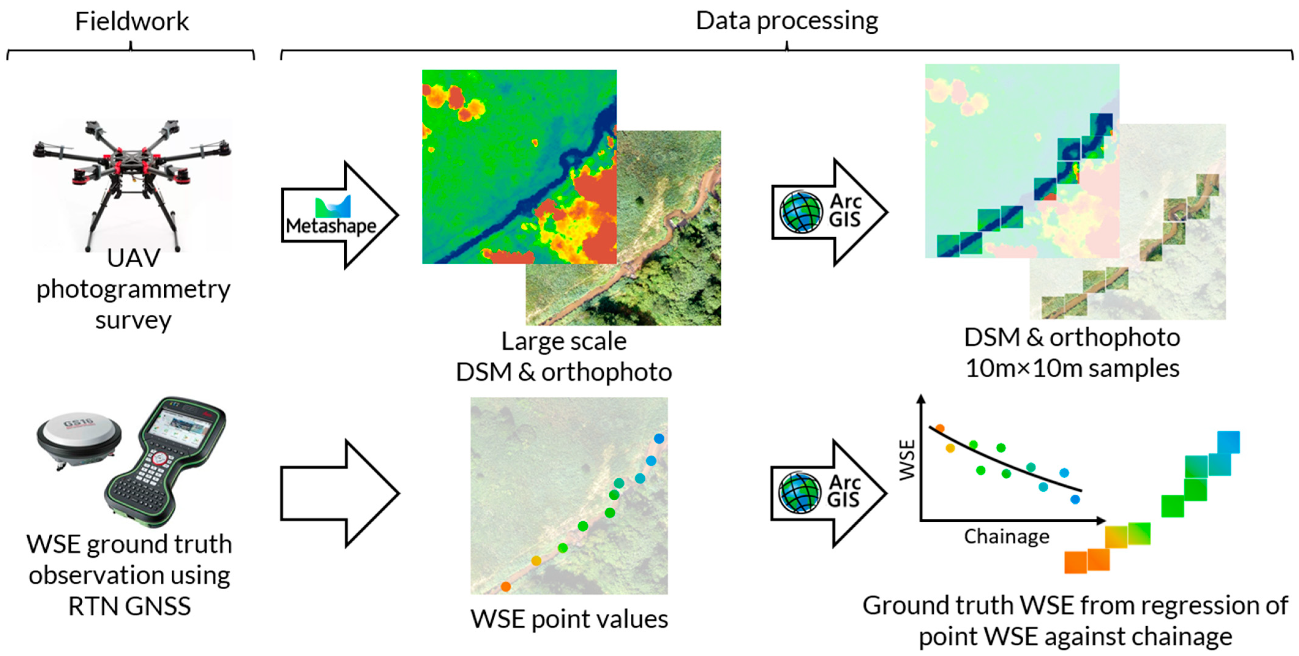
Figure 3 shows a data set preparation workflow that includes both fieldwork and data processing.
2.4. Machine Learning Data Set Structure
The machine learning data set comprises 322 samples. For details on the number of samples in each subset, see Table 1. Every sample includes the data described below.
- Photogrammetric orthophoto. A square crop of an orthophoto representing area, containing the water body of a stream and adjacent land. A grayscale image is represented as a array of integer values from to (1-channel image of pixels).
- Photogrammetric DSM. A square crop of the DSM representing the same area as the orthophoto sample described above. Stored as array of floating-point numbers containing elevations of pixels expressed in m above MSL (height above mean sea level).
- Water Surface Elevation. Ground truth WSE of the water body segment included in the orthophoto and DSM sample. Represented as a single floating-point value expressed in m above MSL.
- Metadata. The following additional information is stored for each sample:
- ○
- DSM statistics. Mean, standard deviation, minimum, and maximum values of the photogrammetric DSM sample array, which can be used for standardization or normalization. Represented as floating point values expressed in m above MSL.
- ○
- Centroid latitude and longitude. World Geodetic System 8’4 (WGS-84) geographical coordinates of the centroid of the shape of the sample area. Represented as floating-point numbers.
- ○
- Chainage. Sample position expressed using a chainage relative for a given stream section.
- ○
- Subset ID. Text value that identifies the survey subset to which the sample belongs. Available values: “GRO21”, “RYB21”, “GRO20”, “RYB20, “AMO18”. For additional information about case studies, see Section 2.1.
2.5. DSM-WSE Relationship
Figure 4 shows example dataset samples with marked areas where the DSM equals the actual WSE ± 5 cm. It can be seen that the patterns are not straightforward and in places do not meet the rule saying that the water level read from the DSM at the streambank corresponds to the WSE.
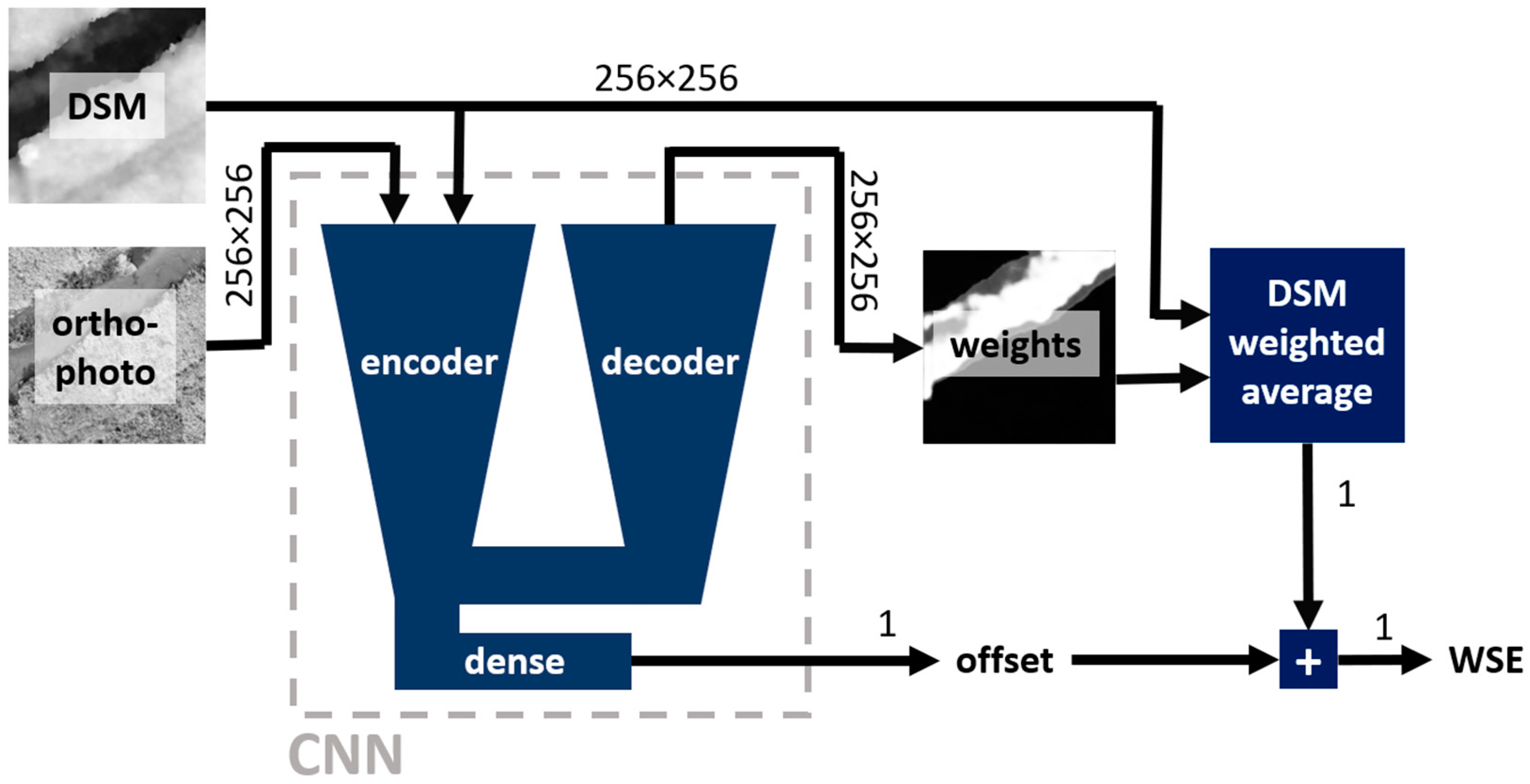
2.6. Deep Learning Framework
In this study, a deep learning (DL) convolutional neural network (CNN) is utilized to estimate a WSE from a DSM and an orthophoto. Two approaches are tested: direct regression of WSE using an encoder and a solution based on the weighted average of the DSM using a weight mask predicted by an autoencoder network. Note that the proposed approaches will be referred to hereafter as “direct regression” and “mask averaging”. Figure 5 and Figure 6 depict schematic representations of the proposed approaches. A third framework, which combines elements from the two mentioned ones, was also tested. However, it did not yield significantly improved results. Further details can be found in Appendix B.
All CNN models used in this study were configured to incorporate two input channels (DSM and grayscale orthophoto). In all approaches, training is conducted using mean squared error (MSE) loss. This implies that in the mask-averaging approach, no ground truth masks were employed for training. Instead, the network autonomously learns to determine the optimal weight mask through the optimization of the MSE loss. CNN architectures originally designed for semantic segmentation were employed to generate weight masks. They were configured to generate single-channel predictions. By employing the sigmoid activation function at the output of the model, the model generates weight masks with values ranging between 0 and 1. All of the autoencoder architectures used in this study were sourced from the Segmentation Models Pytorch library [37].
All the training was performed with a learning rate of 10−5 using the Adam optimizer. Training was undertaken until the RMSE on the validation subset showed no further reduction for the next 20 learning epochs. Given that batch size has a notable impact on accuracy, various values of it were tested during the exploration for the optimal model during grid search (refer to Section 2.10).
2.7. Standardization
As the DSM and orthophoto arrays have values from different ranges and distributions, they are subjected to feature scaling before they are fed into the CNN model in order to ensure proper convergence of the gradient iterative algorithm during training [38]. The DSMs were standardized according to the equation:
where:
- —standardized sample DSM two-dimensional (2D) array with values centered around 0;
- —raw sample DSM 2D array with values expressed in ;
- —mean DSM value of a sample;
- —standard deviation of DSM arrays pixel values for the entire data set.
This method of standardization has two advantages. Firstly, by subtracting the average value of a sample, standardized DSMs are always centered around zero, so the algorithm is insensitive to absolute altitude differences between case studies. Actual WSE relative to mean sea level can be recovered by inverse standardization. Secondly, dividing all samples by the same value of the entire data set ensures that all standardized samples are scaled equally. It was experimentally found during preliminary model tests that multiplying the denominator by 2 results in better model accuracy compared to standardization that does not include this factor.
Orthophotos were standardized using ImageNet [39] data set mean and standard deviation according to the equation:
where:
- —standardized 1-channel orthophoto gray-scale image (2D array) with values centered around 0;
- —1-channel orthophoto gray-scale image (2D array) represented with values from the range [0, 1];
- —mean value of ImageNet data set red, green and blue channel values means (0.485, 0.456, 0.406);
- —mean value of ImageNet data set red, green, and blue channel values standard deviations (0.229, 0.224, 0.225).
2.8. Augmentation
In order to increase the size of the training data set and therefore improve prediction generalization, each sample array used to train the model was subjected to the following augmentation operations: (i) rotation of 0°, 90°, 180°, or 270° and (ii) no inversion, inversion in the x-axis, inversion in the y-axis, or inversion both in the x-axis and the y-axis. This gives a total of 16 permutations, which makes the training data set 16 times larger.
2.9. Cross Validation
Two variants of the k-fold cross-validation method were employed: one with stratified folds of mixed samples from each case study and another with all-in-case-out folds of isolated samples for each case study.
Stratified folds were generated by selecting for validation samples at intervals of every fifth element from the entire dataset. A total of 5 folds were created. The validation subset in each fold contained a comparable number of samples representing each of the case studies. The illustration in Figure 7 highlights the selection of validation subsets for each of the 5 folds.
In the all-in-case-out variant of k-fold cross-validation, 5 folds were also created. However, in this scenario, a validation subset for each fold contained samples exclusively from one case study, while the remaining samples from the other 4 case studies were utilized for training. This method of cross-validation assesses the model’s ability to generalize, i.e., its capacity to predict from data outside the training data distribution.
2.10. Grid Search
The search for the best configuration of the proposed solutions was carried out using grid search in which all possible combinations of proposed parameters were tested. Propositions of configurations depended on the approach variant. The combinations included different types of encoders, architectures, and batch sizes. The architectures tested were: U-Net [40], MA-Net [41] and PSP-Net [42]. Encoders tested were various depths of the VGG [43] and ResNet [44] encoders. Details on configurations used for each approach are presented in Table 2.
2.11. Centerline and Streambank Sampling
The data acquired in this study allow for the use of straightforward methods for determining WSE through sampling from photogrammetric DSM along the stream centerline and at the streambank [25]. These readings will be used for baseline comparison with the proposed method. The polylines used for sampling were determined manually, without employing any algorithm. Sampling was performed with care, especially in the water-edge method, where attention was given to ensuring that samples were consistently taken from the water area, albeit possibly close to the streambank.
3. Results
3.1. Grid Search Results
During the grid search of optimal parameters, multiple trainings were performed, taking into account various parameters and validation subsets. Detailed statistics of the grid search results are presented in Appendix A. The set of parameters (batch size, encoder, architecture) for which the RMSE achieved on the validation set averaged over all folds (both with stratified and leave-one-case-out cross-validation) was the lowest was chosen as the best configuration. Parameters combinations that achieved the best accuracy as well as their validation RMSEs averaged over all cross-validation folds are shown in Table 3.
3.2. Accuracy Metrics
Accuracy metrics were calculated for all cross-validation methods, case studies, and approach variants. The root mean square error (RMSE), mean absolute error (MAE), and mean bias error (MBE) metrics were used. As a comparison with existing methods using photogrammetric DSM to read WSE in a small stream, the same set of metrics was calculated for values sampled from DSM near the streambank and at the centerline. The results are shown in Table 4, Table 5 and Table 6.
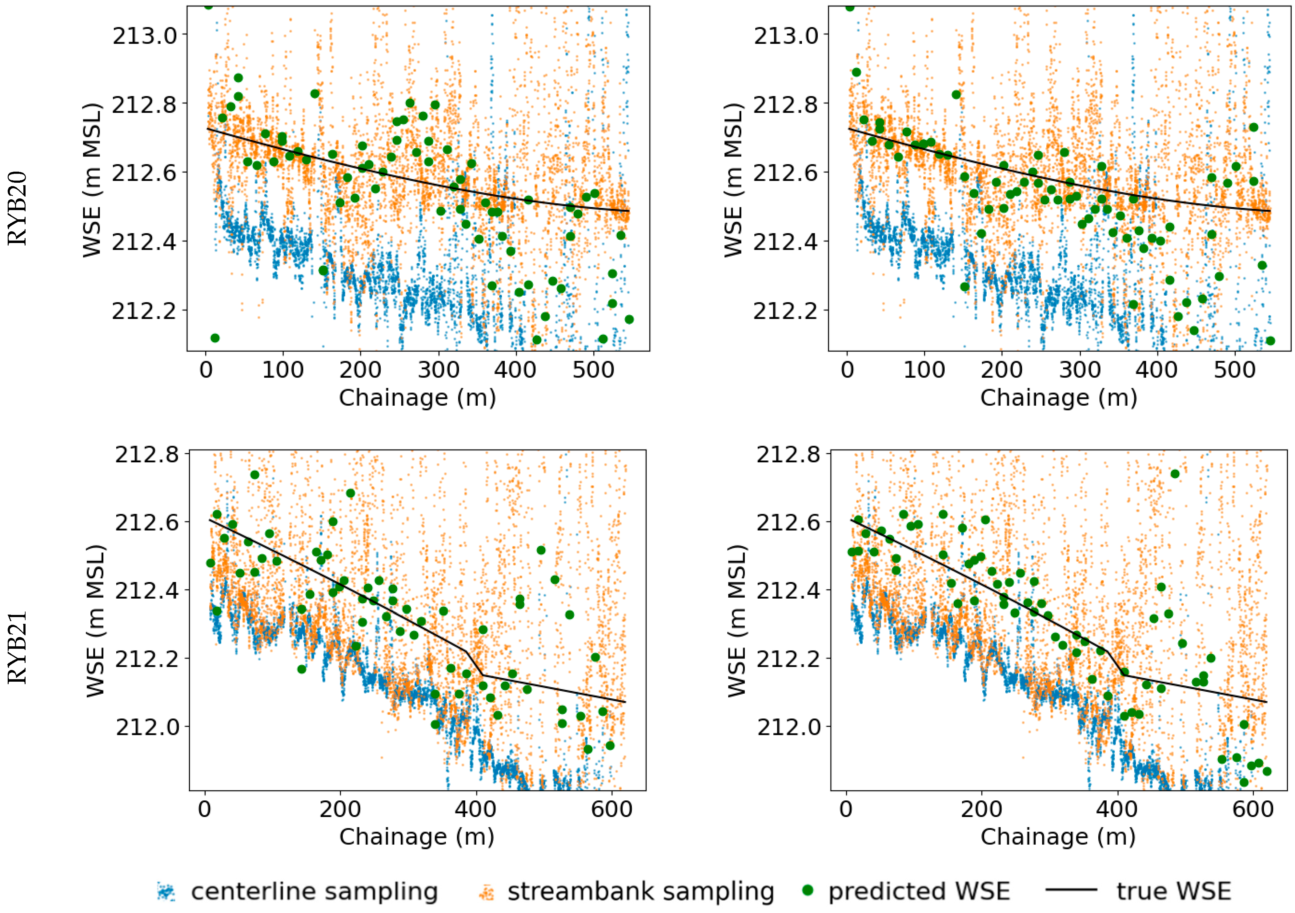
3.3. Plots against Chainage
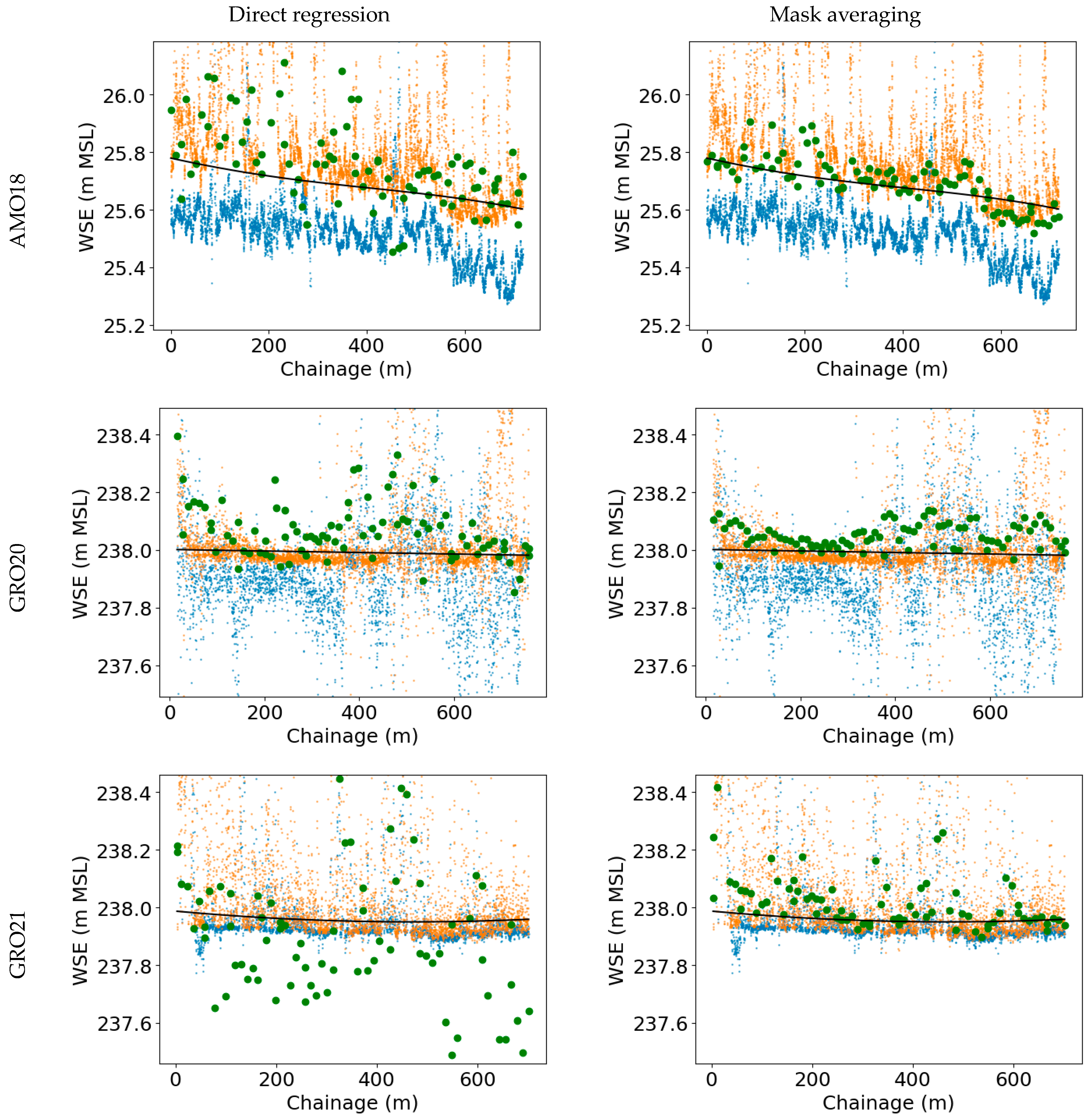
Figure 8 and Figure 9 show WSE predictions as a function of chainage made on validation sets for both stratified and all-in-case-out cross-validation. Predictions are compared with actual WSEs and those obtained from sampling the DSM raster near streambank and at the stream centerline.
Figure 10 shows the residuals (the difference between ground truth and predicted WSE). Residuals are shown as a function of chainage for each case study and method separately. Residuals obtained both during stratified and all-in-case-out cross-validation are included.
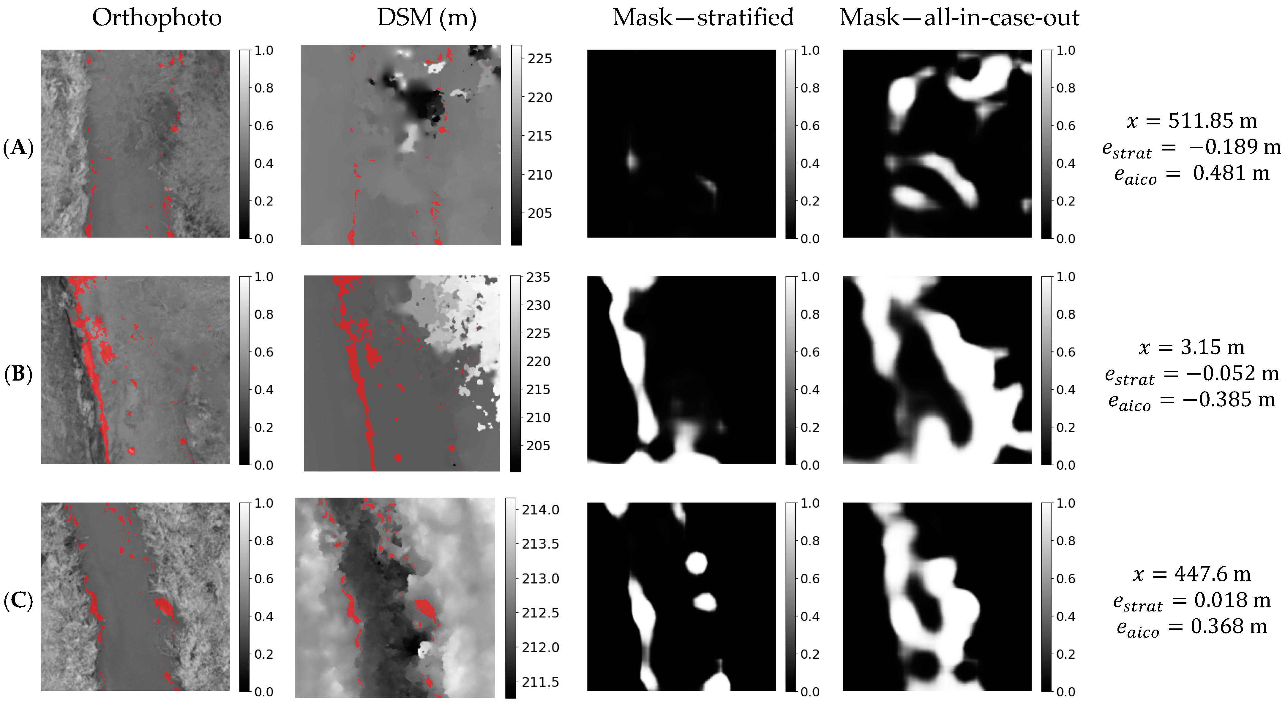
3.4. Weight Masks Visualization
In mask averaging solution predicted weight mask is used to sample WSE value from DSM. In this approach no ground truth masks were used during training and the network autonomously learned to determine the optimal weight mask through the optimization of the MSE loss. It is possible to visualize the mask used to calculate the WSE in mask averaging solution, which contributes enhanced value to the solution, particularly with respect to its explainability.
To depict the nature of the samples that were successfully addressed by mask averaging solution, three samples characterized by the smallest residuals are showcased for each case study. The orthophoto and DSM samples, alongside weight masks predicted in mask averaging solution, are graphically represented. The results are shown in Figure 11, Figure 12, Figure 13, Figure 14 and Figure 15.
To observe the factors contributing to the reduced accuracy of the proposed solution in specific samples, further analyses were undertaken. For each case study, graphical representations akin to Figure 11, Figure 12, Figure 13, Figure 14 and Figure 15 were generated, featuring the orthophoto and DSM samples, along with the weight masks predicted in the mask-averaging solution. However, in this iteration, the visualizations concentrated on the three samples manifesting the largest residuals for each case study. The outcomes of these analyses are depicted in Figure 16, Figure 17, Figure 18, Figure 19 and Figure 20.
4. Discussion
4.1. Discussion of Straightforward Sampling of DSM
In comparing methods based on straightforward DSM sampling along the centerline and near streambank, the RMSE obtained by the centerline method is better than that obtained by the streambank method (Table 4). Conversely, regarding MAE, the situation is reversed: the MAE obtained by the centerline method is worse than that obtained by the streambank method (Table 5). As RMSE, in contrast to MAE, emphasizes outliers, it suggests that the streambank method is more likely to exhibit measurement outliers. This could be attributed to sampling DSM values near the bank vegetation that can influence the measurement. This aligns with the introduction’s assertion that the streambank method is suitable only for gently sloping banks without vegetation.
Both the streambank and centerline methods exhibit bias, as indicated by the MBE metric (Table 6). The centerline method shows an average negative bias of approximately 13 cm, implying an underestimation of water levels compared to the actual levels. Conversely, the streambank method demonstrates an average positive bias of about 9 cm, indicating an overestimation of water levels. The centerline method’s underestimation might be attributed to light penetrating below the water table, causing the DSM to register a lower level than the actual water table. The overestimation in the streambank method further supports the impact of steep streambanks and tall plants near the points where water levels were sampled.
4.2. Impact of Cross-Validation Method
The evaluation of the proposed methods involves the utilization of two distinct cross-validation approaches, each serving a specific purpose. Stratified cross-validation provides insights into the model’s capacity to learn from data across all available case studies and apply this acquired knowledge to predict samples not included in the training set but originating from the same case studies used during training. In contrast, the all-in-case-out cross-validation method offers a comprehensive understanding of the model’s generalization capabilities. In this approach, the samples used for training are entirely sourced from different case studies than those used for validation. For instance, in all-in-case-out cross-validation, predictions regarding the Danish Åmose Å case study were made using a model trained exclusively on data from Polish case studies. Accuracy metrics obtained through stratified cross-validation are better than those acquired via the all-in-case-out cross-validation method. This outcome is not surprising considering the nature of each cross-validation method.
4.3. Comparison between Proposed Deep Learning Approaches
The comparison between the approaches proposed in this study, the direct-regression and mask-averaging methods, reveals that the latter decisively outperforms in all cross-validation methods and across all case studies in terms of the RMSE and MAE metrics (Table 4 and Table 5). Regarding the MBE metric, both methods exhibit a low average bias, up to 2 cm, and neither mask averaging nor direct regression demonstrates a significant superiority (Table 6).
The direct-regression and mask-averaging methods differ significantly in terms of the general concept and architectures used. These differences have implications in terms of the network’s propensity for overtraining. In the mask-averaging solution, a mask that considers the unique stream shape is predicted for each sample. This compels the network to treat each sample individually and forces it to sample water levels from the DSM instead of guessing WSE values remembered by the network during training. This does not apply to the direct-regression solution, as it is not known to what extent the solution samples values from the DSM and to what extent it guesses the WSE based on other features.
Given the significantly better accuracy of the mask-averaging solution over direct regression, and to enhance the clarity of the subsequent analysis, only the mask-averaging method will be compared with the existing methods in the remainder of this discussion section.
4.4. Explainability in the Mask-Averaging Approach
A significant advantage of the mask-averaging solution over direct regression lies in its explainability, as the weight mask used for sampling WSE from DSM can be previewed in this method. Visible in Figure 11, Figure 12, Figure 13, Figure 14 and Figure 15, the masks generated have high weight values for areas near the streambanks. This supports the claim that the DSM represents the value of the WSE near the edges. Nevertheless, the mask-averaging method performs significantly better than manually sampling DSM along the streambank. Several factors contribute to this. First, the generated masks do not have high weights along the entire streambank, presumably ignoring DSM artifacts that could generate outliers. This is particularly evident in the weights generated in stratified cross-validation, where the network had a chance to specialize in the validated case study. In addition, the weights averaging solution does not treat both sides of the river equally. For some cases, we see that the streams bank on the one side of the sample is more favored by the weight mask. The third aspect is that in the mask-averaging method, the samples collected and averaged from wide strips of DSM pixels. In manual sampling, DSM values were collected along a single line and no averaging was performed. Another aspect is that the weighting masks in the mask-averaging method have floating-point values ranging from 0 to 1 so that the network could give different levels of importance to the DSM pixels. All the mentioned features of the mask-averaging method can be encapsulated in the statement that the method is flexible and adapts to the characteristics of a given sample.
Based on an analysis of Figure 16, Figure 17, Figure 18, Figure 19 and Figure 20, one can find reasons for the poor performance of the solution for some samples. The first is the presence of dense vegetation covering the water. Its effect is mainly seen in Figure 18 for case study GRO21. The second reason is the presence of trees in the sample area. Many of the samples for which a poor result was obtained contain trees, as can be seen particularly in Figure 19 and Figure 20 for the case studies RYB20 and RYB21. It is essential to acknowledge, however, that the outcomes derived from the samples depicted in Figure 16, Figure 17, Figure 18, Figure 19 and Figure 20 represent uncommon outliers, and the provided explanations are not universally applicable. Numerous samples exhibit similar characteristics, such as water surfaces obscured by vegetation and the presence of tree crowns, yet the proposed solution has proficiently determined the WSE for these instances.
4.5. Comparison of Deep Learning Approach with Direct Sampling of DSM
Regardless of the cross-validation method employed, the proposed method consistently outperforms the straightforward sampling of WSE from DSMs at the centerline or streambank (Table 4, Table 5 and Table 6). This applies to all RMSE, MAE, and MBE metrics. Thus, the proposed method unequivocally enhances the potential of using photogrammetric DSMs to determine WSE in small streams.
4.6. Comparison with Other Methods
Table 7 compares the results obtained in this study with those of other UAV-based methods reported by Bandini et al. [25]. All the results presented for comparison use data from the same case study of the Åmose Å stream in Denmark, collected on 21 November 2018. In this comparison, similarly to the results described in Section 4.5, the proposed method significantly outperforms methods using photogrammetry. The proposed method also outperforms the lidar-based method. Compared to the method using radar, the proposed method, validated with the more rigorous all-in-case-out method, is inferior. However, when we consider results from the stratified cross-validation, the proposed method achieves similar results to the radar measurement, with a slightly worse RMSE but surpassing it in the MAE and MBE metrics.
5. Conclusions
In this study, the feasibility of employing deep learning to extract the WSE of a small stream from photogrammetric DSM and orthophoto was investigated. The task proved to be non-trivial, as the most obvious solution of direct regression using an encoder proved to be ineffective. Only a properly adapted architecture, which involved predicting the mask of the weights and then using this for sampling the DSM, obtained a satisfactory result.
The principal steps of the proposed solution encompass the following: (i) Acquiring a photogrammetric survey over the river area and incorporating it into a geographic reference system, for instance, by utilizing ground control points. (ii) Extracting DSM and orthophoto raster samples that encompass the stream area and adjacent land. (iii) Employing a trained model for prediction. Improving accuracy can be achieved by finetuning for a specific case.
The solution was validated using two cross-validation methods: stratified and all-in-case-out. These methods differ in the degree of strictness associated with validation using samples from case studies unavailable to the model during training. Depending on the case study and the level of validation strictness, the proposed solution achieves a RMSE ranging between 2 cm and 16 cm. Compared to methods based on straightforward sampling of photogrammetric DSM, the proposed solution achieves, on average, an 84% lower RMSE for stratified cross-validation and a 62% lower RMSE for all-in-case-out cross-validation. By outperforming current methods based on UAV photogrammetry, the proposed solution substantially amplifies the potential of utilizing UAV photogrammetry for WSE estimation.
By utilizing data from another study, the proposed solution was compared on the same case study with other UAV-based methods. For that case study, the proposed solution achieved an RMSE score of 5.9 cm for all-in-case-out cross-validation and 3.5 cm for stratified cross-validation, which is close to the result achieved by the radar-based method (RMSE of 3 cm), which is considered the most accurate method available. The proposed solution has a high level of flexibility and generalizability, making satisfactory predictions for data from case studies not available during training. Another feature of the solution is its explainability, as the masks serving an intermediate function in the prediction process provide interesting information about the areas of the DSM that correctly represent the WSE.
Despite the advantages of using UAVs for WSE surveys such as the ability to operate in inaccessible terrain and obtain spatially distributed measurements, one must be aware of some limitations hindering the use of UAVs related to adverse weather conditions (strong winds, precipitation, or fog), flight restrictions over certain zones due to aviation regulations, or the greater complexity of data processing.
Author Contributions
Conceptualization, R.S.; methodology, R.S., P.Ć., P.W., M.Z. and M.P.; software, R.S. and M.P.; validation, R.S., P.Ć., P.W., M.Z. and M.P.; formal analysis, M.Z., P.W. and M.P.; investigation, R.S., M.Z., P.W., M.P. and P.Ć.; resources, P.W., M.Z., P.Ć. and M.P.; data curation, R.S. and M.Z.; writing—original draft preparation, R.S.; writing—review and editing, R.S., P.W., M.Z., M.P. and P.Ć.; visualization, R.S.; supervision, M.Z., P.W. and M.P.; project administration, P.W. and M.Z.; funding acquisition, P.W. and M.Z. All authors have read and agreed to the published version of the manuscript.
Funding
This research was funded by National Science Centre, Poland, project WATERLINE (2020/02/Y/ST10/00065), under the CHISTERA IV program of the EU Horizon 2020 (grant no 857925) and the “Excellence Initiative—Research University” program at the AGH University of Science and Technology.
Data Availability Statement
Geospatial raster and shape files used in the study are available online in the Zenodo repository (https://doi.org/10.5281/zenodo.7185594). The source codes and the preprocessed machine learning data set are available online in the github repository (https://github.com/radekszostak/stream-wse-uav-ml, accessed on 27 January 2024).
Acknowledgments
We gratefully acknowledge the Polish high-performance computing infrastructure PLGrid (HPC Centers: ACK Cyfronet AGH) for providing computer facilities and support within computational grant no. PLG/2023/016833.
Conflicts of Interest
The authors declare no conflicts of interest.
Abbreviations
| 2D | two-dimensional |
| AMO18 | Åmose Å 2018 case study |
| CNN | convolutional neural network |
| DL | deep learning |
| DSM | digital surface model |
| GCP | ground control point |
| GNSS | global navigation satellite system |
| GRO20 | Grodzisko 2020 case study |
| GRO21 | Grodzisko 2021 case study |
| MAE | mean absolute error |
| MBE | mean bias error |
| ML | machine learning |
| MSL | height above mean sea level |
| RMSE | root mean square error |
| RTN | real-time network |
| RYB20 | Rybna 2020 case study |
| RYB21 | Rybna 2021 case study |
| SFM | structure from motion |
| St. Dev. | standard deviation |
| UAV | unmanned aerial vehicle |
| WGS-84 | World Geodetic System 8’4 |
| WS | water surface |
| WSE | water surface elevation |
Appendix A. Grid Search Statistics
Detailed statistics on the RMSE results that the various configurations tested achieved on the validation set during the grid search are shown in Figure A1, Figure A2, Figure A3, Figure A4 and Figure A5.
Figure A1.
Direct regression—validation RMSEs achieved in different cross-validation folds by each encoder. The error bars, indicating 95th percentile intervals, result from variations in batch sizes tested during experimentation.
Figure A1.
Direct regression—validation RMSEs achieved in different cross-validation folds by each encoder. The error bars, indicating 95th percentile intervals, result from variations in batch sizes tested during experimentation.

Figure A2.
Direct regression—validation RMSEs achieved in different cross-validation folds by various batch sizes. The error bars, indicating 95th percentile intervals, result from variations in encoders tested during experimentation.
Figure A2.
Direct regression—validation RMSEs achieved in different cross-validation folds by various batch sizes. The error bars, indicating 95th percentile intervals, result from variations in encoders tested during experimentation.

Figure A3.
Mask averaging—validation RMSEs achieved in different cross-validation folds by various encoders. The error bars, indicating 95th percentile intervals, result from variations in batch sizes and architectures tested during experimentation.
Figure A3.
Mask averaging—validation RMSEs achieved in different cross-validation folds by various encoders. The error bars, indicating 95th percentile intervals, result from variations in batch sizes and architectures tested during experimentation.

Figure A4.
Mask averaging—validation RMSEs achieved in different cross-validation folds by various batch sizes. The error bars, indicating 95th percentile intervals, result from variations in encoders and architectures tested during experimentation.
Figure A4.
Mask averaging—validation RMSEs achieved in different cross-validation folds by various batch sizes. The error bars, indicating 95th percentile intervals, result from variations in encoders and architectures tested during experimentation.

Figure A5.
Mask averaging—validation RMSEs achieved in different cross-validation folds using various architectures. The error bars, indicating 95th percentile intervals, result from variations in batch sizes and encoders tested during experimentation.
Figure A5.
Mask averaging—validation RMSEs achieved in different cross-validation folds using various architectures. The error bars, indicating 95th percentile intervals, result from variations in batch sizes and encoders tested during experimentation.

Appendix B. Unsuccessful Approach
A third solution aimed at further improving the mask-averaging approach has been tested. It was a fusion of the two solutions proposed in the main text. Although it was more complex, it achieved a worse result than the weighted-averaging approach.
In the fusion solution, the encoder predicts a correction in the form of an offset added to the weighted average of DSM calculated using the predicted weight mask. Figure A6 depict schematic representations of this approach.
Figure A6.
Fusion approach—schematic representation. Numbers near the arrows provide information about the dimensions of the flowing data.
Figure A6.
Fusion approach—schematic representation. Numbers near the arrows provide information about the dimensions of the flowing data.

During grid search, the same propositions of configurations as in the mask-averaging approach were tested, i.e., U-Net, MA-Net, PSP-Net architectures, VGG13, VGG16, VGG19 encoders, and the batch sizes 1, 2, 4, 8, and 16. The best combination was the PSP-Net architecture with a VGG19 encoder trained using a batch size of 2. It achieved a validation RMSE averaged over all cross-validation folds equal to 0.079 m. As a reminder, the mask-averaging approach achieved an analogous result equal to 0.070 m.
References
- IPCC. Climate Change 2014: Synthesis Report; Intergovernmental Panel on Climate Change: Geneva, Switzerland, 2015; ISBN 978-92-9169-143-2. [Google Scholar]
- UNESCO. The United Nations World Water Development Report 2020: Water and Climate Change; United Nations Educational, Scientific and Cultural Organization: Paris, France, 2020; ISBN 978-92-3-100371-4. [Google Scholar]
- Blöschl, G.; Bierkens, M.F.P.; Chambel, A.; Cudennec, C.; Destouni, G.; Fiori, A.; Kirchner, J.W.; McDonnell, J.J.; Savenije, H.H.G.; Sivapalan, M.; et al. Twenty-Three Unsolved Problems in Hydrology (UPH)—A Community Perspective. Hydrol. Sci. J. 2019, 64, 1141–1158. [Google Scholar] [CrossRef]
- Alsdorf, D.E.; Rodríguez, E.; Lettenmaier, D.P. Measuring Surface Water from Space. Rev. Geophys. 2007, 45, 2006RG000197. [Google Scholar] [CrossRef]
- Jarihani, A.A.; Callow, J.N.; Johansen, K.; Gouweleeuw, B. Evaluation of Multiple Satellite Altimetry Data for Studying Inland Water Bodies and River Floods. J. Hydrol. 2013, 505, 78–90. [Google Scholar] [CrossRef]
- Domeneghetti, A. On the Use of SRTM and Altimetry Data for Flood Modeling in Data-Sparse Regions. Water Resour. Res. 2016, 52, 2901–2918. [Google Scholar] [CrossRef]
- Langhammer, J.; Bernsteinová, J.; Miřijovský, J. Building a High-Precision 2D Hydrodynamic Flood Model Using UAV Photogrammetry and Sensor Network Monitoring. Water 2017, 9, 861. [Google Scholar] [CrossRef]
- Montesarchio, V.; Napolitano, F.; Rianna, M.; Ridolfi, E.; Russo, F.; Sebastianelli, S. Comparison of Methodologies for Flood Rainfall Thresholds Estimation. Nat. Hazards 2014, 75, 909–934. [Google Scholar] [CrossRef]
- Tarpanelli, A.; Barbetta, S.; Brocca, L.; Moramarco, T. River Discharge Estimation by Using Altimetry Data and Simplified Flood Routing Modeling. Remote Sens. 2013, 5, 4145–4162. [Google Scholar] [CrossRef]
- Jiang, L.; Bandini, F.; Smith, O.; Jensen, I.K.; Bauer-Gottwein, P. The Value of Distributed High-Resolution UAV-Borne Observations of Water Surface Elevation for River Management and Hydrodynamic Modeling. Remote Sens. 2020, 12, 1171. [Google Scholar] [CrossRef]
- Lawford, R.; Strauch, A.; Toll, D.; Fekete, B.; Cripe, D. Earth Observations for Global Water Security. Curr. Opin. Environ. Sustain. 2013, 5, 633–643. [Google Scholar] [CrossRef]
- Shiklomanov, A.I.; Lammers, R.B.; Vörösmarty, C.J. Widespread Decline in Hydrological Monitoring Threatens Pan-Arctic Research. EoS Trans. Am. Geophys. Union 2002, 83, 13–17. [Google Scholar] [CrossRef]
- McCabe, M.F.; Rodell, M.; Alsdorf, D.E.; Miralles, D.G.; Uijlenhoet, R.; Wagner, W.; Lucieer, A.; Houborg, R.; Verhoest, N.E.C.; Franz, T.E.; et al. The Future of Earth Observation in Hydrology. Hydrol. Earth Syst. Sci. 2017, 21, 3879–3914. [Google Scholar] [CrossRef]
- Cracknell, A.P. The Development of Remote Sensing in the Last 40 Years. Int. J. Remote Sens. 2018, 39, 8387–8427. [Google Scholar] [CrossRef]
- Zhao, Q.; Yu, L.; Du, Z.; Peng, D.; Hao, P.; Zhang, Y.; Gong, P. An Overview of the Applications of Earth Observation Satellite Data: Impacts and Future Trends. Remote Sens. 2022, 14, 1863. [Google Scholar] [CrossRef]
- Louet, J.; Bruzzi, S. ENVISAT Mission and System. In Proceedings of the IEEE 1999 International Geoscience and Remote Sensing Symposium. IGARSS’99 (Cat. No.99CH36293), Hamburg, Germany, 28 June–2 July 1999; IEEE: Piscataway, NJ, USA, 1999; Volume 3, pp. 1680–1682. [Google Scholar]
- Donlon, C.; Berruti, B.; Buongiorno, A.; Ferreira, M.-H.; Féménias, P.; Frerick, J.; Goryl, P.; Klein, U.; Laur, H.; Mavrocordatos, C.; et al. The Global Monitoring for Environment and Security (GMES) Sentinel-3 Mission. Remote Sens. Environ. 2012, 120, 37–57. [Google Scholar] [CrossRef]
- Kittel, C.M.M.; Jiang, L.; Tøttrup, C.; Bauer-Gottwein, P. Sentinel-3 Radar Altimetry for River Monitoring—A Catchment-Scale Evaluation of Satellite Water Surface Elevation from Sentinel-3A and Sentinel-3B. Hydrol. Earth Syst. Sci. 2021, 25, 333–357. [Google Scholar] [CrossRef]
- Sulistioadi, Y.B.; Tseng, K.-H.; Shum, C.K.; Hidayat, H.; Sumaryono, M.; Suhardiman, A.; Setiawan, F.; Sunarso, S. Satellite Radar Altimetry for Monitoring Small Rivers and Lakes in Indonesia. Hydrol. Earth Syst. Sci. 2015, 19, 341–359. [Google Scholar] [CrossRef]
- Pavelsky, T.M.; Durand, M.T.; Andreadis, K.M.; Beighley, R.E.; Paiva, R.C.D.; Allen, G.H.; Miller, Z.F. Assessing the Potential Global Extent of SWOT River Discharge Observations. J. Hydrol. 2014, 519, 1516–1525. [Google Scholar] [CrossRef]
- Biancamaria, S.; Lettenmaier, D.P.; Pavelsky, T.M. The SWOT Mission and Its Capabilities for Land Hydrology. Surv. Geophys. 2016, 37, 307–337. [Google Scholar] [CrossRef]
- Strahler, A.N. Quantitative Analysis of Watershed Geomorphology. Eos Trans. Am. Geophys. Union 1957, 38, 913. [Google Scholar] [CrossRef]
- Wohl, E. The Significance of Small Streams. Front. Earth Sci. 2017, 11, 447–456. [Google Scholar] [CrossRef]
- Vélez-Nicolás, M.; García-López, S.; Barbero, L.; Ruiz-Ortiz, V.; Sánchez-Bellón, Á. Applications of Unmanned Aerial Systems (UASs) in Hydrology: A Review. Remote Sens. 2021, 13, 1359. [Google Scholar] [CrossRef]
- Bandini, F.; Sunding, T.P.; Linde, J.; Smith, O.; Jensen, I.K.; Köppl, C.J.; Butts, M.; Bauer-Gottwein, P. Unmanned Aerial System (UAS) Observations of Water Surface Elevation in a Small Stream: Comparison of Radar Altimetry, LIDAR and Photogrammetry Techniques. Remote Sens. Environ. 2020, 237, 111487. [Google Scholar] [CrossRef]
- Bühler, Y.; Adams, M.S.; Stoffel, A.; Boesch, R. Photogrammetric Reconstruction of Homogenous Snow Surfaces in Alpine Terrain Applying Near-Infrared UAS Imagery. Int. J. Remote Sens. 2017, 38, 3135–3158. [Google Scholar] [CrossRef]
- Ouédraogo, M.M.; Degré, A.; Debouche, C.; Lisein, J. The Evaluation of Unmanned Aerial System-Based Photogrammetry and Terrestrial Laser Scanning to Generate DEMs of Agricultural Watersheds. Geomorphology 2014, 214, 339–355. [Google Scholar] [CrossRef]
- Kasvi, E.; Salmela, J.; Lotsari, E.; Kumpula, T.; Lane, S.N. Comparison of Remote Sensing Based Approaches for Mapping Bathymetry of Shallow, Clear Water Rivers. Geomorphology 2019, 333, 180–197. [Google Scholar] [CrossRef]
- Woodget, A.S.; Carbonneau, P.E.; Visser, F.; Maddock, I.P. Quantifying Submerged Fluvial Topography Using Hyperspatial Resolution UAS Imagery and Structure from Motion Photogrammetry. Earth Surf. Process. Landf. 2014, 40, 47–64. [Google Scholar] [CrossRef]
- Javernick, L.; Brasington, J.; Caruso, B. Modeling the Topography of Shallow Braided Rivers Using Structure-from-Motion Photogrammetry. Geomorphology 2014, 213, 166–182. [Google Scholar] [CrossRef]
- Pai, H.; Malenda, H.F.; Briggs, M.A.; Singha, K.; González-Pinzón, R.; Gooseff, M.N.; Tyler, S.W. Potential for Small Unmanned Aircraft Systems Applications for Identifying Groundwater-Surface Water Exchange in a Meandering River Reach. Geophys. Res. Lett. 2017, 44, 11868–11877. [Google Scholar] [CrossRef]
- Pugliese, R.; Regondi, S.; Marini, R. Machine Learning-Based Approach: Global Trends, Research Directions, and Regulatory Standpoints. J. Inf. Technol. Data Manag. 2021, 4, 19–29. [Google Scholar] [CrossRef]
- Chen, J.; Liu, H. Laboratory Water Surface Elevation Estimation Using Image-Based Convolutional Neural Networks. Ocean Eng. 2022, 248, 110819. [Google Scholar] [CrossRef]
- Elkhrachy, I. Flash Flood Water Depth Estimation Using SAR Images, Digital Elevation Models, and Machine Learning Algorithms. Remote Sens. 2022, 14, 440. [Google Scholar] [CrossRef]
- Bandini, F.; Sunding, T.P.; Linde, J.; Smith, O.; Jensen, I.K.; Köppl, C.J.; Butts, M.; Bauer-Gottwein, P. Dataset Used in “Unmanned Aerial System (UAS) Observations of Water Surface Elevation in a Small Stream: Comparison of Radar Altimetry, LIDAR and Photogrammetry Techniques”; Licensed under Creative Commons Attribution 2.0 Generic; Zenodo: Geneva, Switzerland, 2019. [Google Scholar]
- Siegel, A.F. Correlation and Regression. In Practical Business Statistics; Elsevier: Amsterdam, The Netherlands, 2016; pp. 299–354. [Google Scholar]
- Iakubovskii, P. Segmentation Models Pytorch v0.3.3; GitHub: San Francisco, CA, USA, 2019. [Google Scholar]
- Wan, X. Influence of Feature Scaling on Convergence of Gradient Iterative Algorithm. J. Phys. Conf. Ser. 2019, 1213, 032021. [Google Scholar] [CrossRef]
- Deng, J.; Dong, W.; Socher, R.; Li, L.-J.; Li, K.; Fei-Fei, L. ImageNet: A Large-Scale Hierarchical Image Database; IEEE: Piscataway, NJ, USA, 2009. [Google Scholar]
- Ronneberger, O.; Fischer, P.; Brox, T. U-net: Convolutional Networks for Biomedical Image Segmentation. arXiv 2015, arXiv:1505.04597. [Google Scholar] [CrossRef]
- Fan, T.; Wang, G.; Li, Y.; Wang, H. MA-Net: A Multi-Scale Attention Network for Liver and Tumor Segmentation. IEEE Access 2020, 8, 179656–179665. [Google Scholar] [CrossRef]
- Zhao, H.; Shi, J.; Qi, X.; Wang, X.; Jia, J. Pyramid Scene Parsing Network. arXiv 2015, arXiv:1612.01105. [Google Scholar] [CrossRef]
- Simonyan, K.; Zisserman, A. Very Deep Convolutional Networks for Large-Scale Image Recognition. arXiv 2015, arXiv:1409.1556, 2014 2015. [Google Scholar]
- He, K.; Zhang, X.; Ren, S.; Sun, J. Deep Residual Learning for Image Recognition. arXiv 2015, arXiv:1512.03385. [Google Scholar] [CrossRef]
Figure 1.
Orthophoto mosaics from Grodzisko (a) and Rybna (b) case studies from 13 July 2021.

Figure 2.
Part of the Kocinka stretch in Rybna (March 2022).

Figure 3.
Schematic representation of the data set preparation workflow. Colors are for illustration purposes only and do not reflect actual data.
Figure 3.
Schematic representation of the data set preparation workflow. Colors are for illustration purposes only and do not reflect actual data.

Figure 4.
Example DSM and orthophoto dataset samples (a–d) with marked areas where the DSM equals the actual WSE ± 5 cm (red color).
Figure 4.
Example DSM and orthophoto dataset samples (a–d) with marked areas where the DSM equals the actual WSE ± 5 cm (red color).

Figure 5.
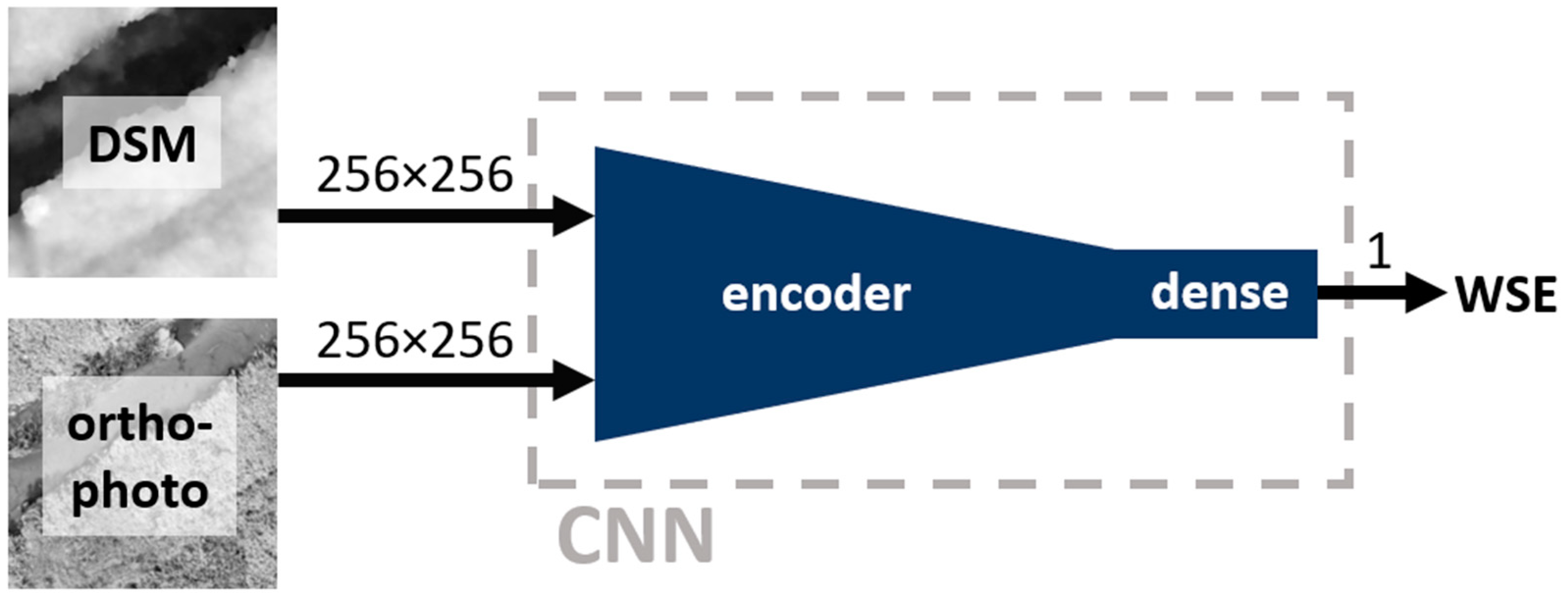
Direct regression approach—schematic representation. Numbers near arrows provide information about the dimensions of the flowing data.
Figure 5.
Direct regression approach—schematic representation. Numbers near arrows provide information about the dimensions of the flowing data.

Figure 6.
Mask averaging approach—schematic representation. Numbers near arrows provide information about the dimensions of the flowing data.
Figure 6.
Mask averaging approach—schematic representation. Numbers near arrows provide information about the dimensions of the flowing data.

Figure 7.
The selection of validation samples for each of the 5 folds in stratified resampling.

Figure 8.
Predictions of validation subsets from stratified cross-validation plotted against chainage (dark-green points). Compared with ground truth WSE (black line), DSM sampled near streambank (orange points), and DSM sampled at stream centerline (blue points). Columns denote different approaches and rows correspond to distinct case studies.


Figure 9.
Predictions of validation subsets from all-in-case-out cross-validation plotted against chainage (dark-green points). Compared with ground truth WSE (black line), DSM sampled near streambank (orange points), and DSM sampled at stream centerline (blue points). Columns denote different approaches and rows correspond to distinct case studies.


Figure 10.
Residuals (ground truth WSE minus predicted WSE) obtained during stratified and all-in-case-out cross-validations for each case study (rows) and method (columns) plotted against chainage.
Figure 10.
Residuals (ground truth WSE minus predicted WSE) obtained during stratified and all-in-case-out cross-validations for each case study (rows) and method (columns) plotted against chainage.

Figure 11.
Orthophoto, DSM, and weight masks obtained in stratified and all-in-case-out cross validations for the three best performing samples from the AMO18 case study. , , and correspond to chainage and residuals obtained using stratified and all-in-case-out cross-validation, respectively. Areas where the DSM equals the actual WSE ± 5 cm are marked in red on the orthophoto and DSM. (A–C) samples ordered from most to least performing.

Figure 12.
Orthophoto, DSM, and masks obtained in stratified and all-in-case-out cross validations for the three best performing samples from the GRO20 case study. , , and correspond to chainage and residuals obtained using stratified and all-in-case-out cross-validation, respectively. Areas where the DSM equals the actual WSE ± 5 cm are marked in red on the orthophoto and DSM. (A–C) samples ordered from most to least performing.

Figure 13.
Orthophoto, DSM, and masks obtained in stratified and all-in-case-out cross validations for the three best performing samples from the GRO21 case study. , and correspond to chainage and residuals obtained using stratified and all-in-case-out cross-validation, respectively. Areas where the DSM equals the actual WSE ± 5 cm are marked in red on the orthophoto and DSM. (A–C) samples ordered from most to least performing.

Figure 14.
Orthophoto, DSM, and masks obtained in stratified and all-in-case-out cross validations for the three best performing samples from the RYB20 case study. , and correspond to chainage and residuals obtained using stratified and all-in-case-out cross-validation, respectively. Areas where the DSM equals the actual WSE ± 5 cm are marked in red on the orthophoto and DSM. (A–C) samples ordered from most to least performing.

Figure 15.
Orthophoto, DSM, and masks obtained in stratified and all-in-case-out cross validations for the three best performing samples from the RYB21 case study. and correspond to chainage and residuals obtained using stratified and all-in-case-out cross-validation, respectively. Areas where the DSM equals the actual WSE ± 5 cm are marked in red on the orthophoto and DSM. (A–C) samples ordered from most to least performing.

Figure 16.
Orthophoto, DSM, and masks obtained in stratified and all-in-case-out cross validations for the three worst performing samples from the AMO18 case study. , and correspond to chainage and residuals obtained using stratified and all-in-case-out cross-validation, respectively. Areas where the DSM equals the actual WSE ± 5 cm are marked in red on the orthophoto and DSM. (A–C) samples ordered from least to most performing.

Figure 17.
Orthophoto, DSM, and masks obtained in stratified and all-in-case-out cross validations for the three worst performing samples from the GRO20 case study. , , and correspond to chainage and residuals obtained using stratified and all-in-case-out cross-validation, respectively. Areas where the DSM equals the actual WSE ± 5 cm are marked in red on the orthophoto and DSM. (A–C) samples ordered from least to most performing.

Figure 18.
Orthophoto, DSM, and masks obtained in stratified and all-in-case-out cross validations for the three worst performing samples from the GRO21 case study. , , and correspond to chainage and residuals obtained using stratified and all-in-case-out cross-validation, respectively. Areas where the DSM equals the actual WSE ± 5 cm are marked in red color on the orthophoto and DSM. (A–C) samples ordered from least to most performing.

Figure 19.
Orthophoto, DSM, and masks obtained in stratified and all-in-case-out cross validations for the three worst performing samples from the RYB20 case study. , , and correspond to chainage and residuals obtained using stratified and all-in-case-out cross-validation, respectively. Areas where the DSM equals the actual WSE ± 5 cm are marked in red on the orthophoto and DSM. (A–C) samples ordered from least to most performing.

Figure 20.
Orthophoto, DSM, and masks obtained in stratified and all-in-case-out cross validations for the three worst performing samples from the RYB21 case study. , , and correspond to chainage and residuals obtained using stratified and all-in-case-out cross-validation, respectively. Areas where the DSM equals the actual WSE ± 5 cm are marked in red on the orthophoto and DSM. (A–C) samples ordered from least to most performing.


Table 1.
Number of WSE point measurements, standard error of estimate for ground truth WSE, and number of extracted data set samples for each case study.
Table 1.
Number of WSE point measurements, standard error of estimate for ground truth WSE, and number of extracted data set samples for each case study.
| Subset ID | Number of WSE Point Measurements | Standard Error of Estimate for Ground Truth WSE (m) | Number of Extracted Data Set Samples |
|---|---|---|---|
| GRO21 | 36 | 0.012 | 64 |
| RYB21 | 52 | 0.013 | 55 |
| GRO20 | 84 | 0.020 | 72 |
| RYB20 | 76 | 0.016 | 57 |
| AMO18 | 7235 | 0.020 | 74 |
Table 2.
Propositions of architecture, encoder, and batch size used in grid search.
| Approach | Architectures | Encoder | Batch Size |
|---|---|---|---|
| Direct regression | - | ResNet18, ResNet50, VGG11, VGG13, VGG16, VGG19 | 1, 2, 4, 8, 16 |
| Mask averaging | U-Net, MA-Net, PSP-Net | VGG13, VGG16, VGG19 | 1, 2, 4, 8, 16 |
Table 3.
Best parameters configurations and achieved validation RMSEs averaged over all cross-validation folds.
Table 3.
Best parameters configurations and achieved validation RMSEs averaged over all cross-validation folds.
| Direct | Mask | |
|---|---|---|
| encoder | VGG16 | VGG19 |
| architecture | - | PSPNet |
| batch size | 1 | 4 |
| Mean RMSE | 0.170 | 0.077 |
Table 4.
RMSEs (m) achieved by proposed direct-regression and mask-averaging approaches and by straightforward sampling of DSM over centerline and near streambank. Both stratified and all-in-case-out cross-validation techniques results are given. Provided mean and sample standard deviation are calculated over all case studies.
| Cross-Validation | Stratified | All-In-Case-Out | - | |||
|---|---|---|---|---|---|---|
| Method | Direct | Mask | Direct | Mask | Centerline | Wateredge |
| AMO18 | 0.099 | 0.035 | 0.170 | 0.059 | 0.219 | 0.308 |
| GRO20 | 0.076 | 0.021 | 0.124 | 0.072 | 0.185 | 0.228 |
| GRO21 | 0.107 | 0.058 | 0.243 | 0.117 | 0.27 | 0.277 |
| RYB20 | 0.095 | 0.048 | 0.176 | 0.156 | 0.449 | 0.259 |
| RYB21 | 0.274 | 0.063 | 0.337 | 0.142 | 0.282 | 0.404 |
| Mean | 0.130 | 0.045 | 0.210 | 0.109 | 0.281 | 0.295 |
| Sample St. Dev. | 0.081 | 0.017 | 0.083 | 0.043 | 0.102 | 0.067 |
Table 5.
MAEs (m) achieved by proposed-direct regression and mask-averaging approaches and by straightforward sampling of DSM over centerline and near streambank. Both stratified and all-in-case-out cross-validation techniques results are given. Provided mean and sample standard deviation are calculated over all case studies.
| Cross-Validation | Stratified | All-In-Case-Out | - | |||
|---|---|---|---|---|---|---|
| Method | Direct | Mask | Direct | Mask | Centerline | Wateredge |
| AMO18 | 0.078 | 0.026 | 0.121 | 0.045 | 0.179 | 0.176 |
| GRO20 | 0.059 | 0.015 | 0.091 | 0.06 | 0.139 | 0.104 |
| GRO21 | 0.082 | 0.028 | 0.195 | 0.072 | 0.117 | 0.138 |
| RYB20 | 0.074 | 0.037 | 0.127 | 0.111 | 0.373 | 0.157 |
| RYB21 | 0.169 | 0.045 | 0.154 | 0.096 | 0.249 | 0.276 |
| Mean | 0.092 | 0.030 | 0.138 | 0.077 | 0.211 | 0.17 |
| Sample St. Dev. | 0.044 | 0.011 | 0.039 | 0.027 | 0.103 | 0.065 |
Table 6.
MBEs (m) achieved by proposed direct-regression and mask-averaging approaches and by straightforward sampling of DSM over centerline and near streambank. Both stratified and all-in-case-out cross-validation techniques results are given. Provided mean and sample standard deviation are calculated over all case studies.
| Cross-Validation | Stratified | All-In-Case-Out | - | |||
|---|---|---|---|---|---|---|
| Method | Direct | Mask | Direct | Mask | Centerline | Wateredge |
| AMO18 | 0.008 | −0.007 | −0.084 | −0.015 | −0.149 | 0.161 |
| GRO20 | −0.024 | −0.007 | −0.076 | −0.057 | −0.071 | 0.042 |
| GRO21 | 0.004 | −0.018 | 0.069 | −0.064 | 0.058 | 0.116 |
| RYB20 | −0.013 | 0.002 | 0.042 | 0.059 | −0.277 | 0.036 |
| RYB21 | −0.076 | 0.006 | −0.034 | −0.004 | −0.225 | 0.102 |
| Mean | −0.020 | −0.005 | −0.017 | −0.016 | −0.133 | 0.091 |
| Sample St. Dev. | 0.034 | 0.009 | 0.069 | 0.049 | 0.132 | 0.053 |
Table 7.
RMSE, MAE, and MBE from this study (using the mask-averaging method with both stratified and all-in-case-out cross-validations) compared with Bandini et al. [25] (using radar, photogrammetry, and lidar), arranged by RMSE. All data are from the same case study of the Åmose Å stream in Denmark, collected on 21 November 2018.
| Method | Source | RMSE | MAE | MBE |
|---|---|---|---|---|
| UAV radar | [25] | 0.030 | 0.033 | 0.033 |
| DL photogrammetry (stratified) | This study | 0.035 | 0.026 | −0.007 |
| DL photogrammetry (all-in-case-out) | This study | 0.059 | 0.045 | −0.015 |
| UAV photogrammetry DSM centerline | [25] | 0.164 | 0.150 | −0.151 |
| UAV photogrammetry point cloud | [25] | 0.180 | 0.160 | −0.160 |
| UAV lidar point cloud | [25] | 0.222 | 0.159 | 0.033 |
| UAV lidar DSM centerline | [25] | 0.358 | 0.238 | 0.076 |
| UAV photogrammetry DSM “water-edge” | [25] | 0.450 | 0.385 | 0.385 |
Disclaimer/Publisher’s Note: The statements, opinions and data contained in all publications are solely those of the individual author(s) and contributor(s) and not of MDPI and/or the editor(s). MDPI and/or the editor(s) disclaim responsibility for any injury to people or property resulting from any ideas, methods, instructions or products referred to in the content. |
© 2024 by the authors. Licensee MDPI, Basel, Switzerland. This article is an open access article distributed under the terms and conditions of the Creative Commons Attribution (CC BY) license (https://creativecommons.org/licenses/by/4.0/).
Share and Cite
MDPI and ACS Style
Szostak, R.; Pietroń, M.; Wachniew, P.; Zimnoch, M.; Ćwiąkała, P. Estimation of Small-Stream Water Surface Elevation Using UAV Photogrammetry and Deep Learning. Remote Sens. 2024, 16, 1458. https://doi.org/10.3390/rs16081458
AMA Style
Szostak R, Pietroń M, Wachniew P, Zimnoch M, Ćwiąkała P. Estimation of Small-Stream Water Surface Elevation Using UAV Photogrammetry and Deep Learning. Remote Sensing. 2024; 16(8):1458. https://doi.org/10.3390/rs16081458
Chicago/Turabian StyleSzostak, Radosław, Marcin Pietroń, Przemysław Wachniew, Mirosław Zimnoch, and Paweł Ćwiąkała. 2024. "Estimation of Small-Stream Water Surface Elevation Using UAV Photogrammetry and Deep Learning" Remote Sensing 16, no. 8: 1458. https://doi.org/10.3390/rs16081458
Note that from the first issue of 2016, this journal uses article numbers instead of page numbers. See further details here.