A Metadata-Enhanced Deep Learning Method for Sea Surface Height and Mesoscale Eddy Prediction

Abstract

Predicting the mesoscale eddies in the ocean is crucial for advancing our understanding of the ocean and climate systems. Establishing spatio-temporal correlation among input data is a significant challenge in mesoscale eddy prediction tasks, especially for deep learning techniques. In this paper, we first present a deep learning solution based on a video prediction model to capture the spatio-temporal correlation and predict future sea surface height data accurately. To enhance the performance of the model, we introduced a novel metadata embedding module that utilizes neural networks to fuse remote sensing metadata with input data, resulting in increased accuracy. To the best of our knowledge, our model outperforms the state-of-the-art method for predicting sea level anomalies. Consequently, a mesoscale eddy detection algorithm will be applied to the predicted sea surface height data to generate mesoscale eddies in future. The proposed solution achieves competitive results, indicating that the prediction error for the eddy center position is 5.6 km for a 3-day prediction and 13.6 km for a 7-day prediction.

1. Introduction

Mesoscale eddies, which are widespread in the global ocean, exhibit circular motions of water masses with horizontal scales ranging from tens to hundreds of kilometers and lifetimes lasting from weeks to months. These eddies play a pivotal role in the transport of heat, salt, nutrients, carbon, and biological organisms across various regions, significantly influencing ocean circulation, mixing, and air–sea interactions [1,2,3]. Consequently, they have far-reaching implications for the climate system and marine ecosystems. It is essential to understand the future locations and properties of mesoscale eddies to enhance ocean modeling, management, and the evaluation of their impact on marine ecosystems and the global climate.

Mesoscale eddy prediction is a challenging task. In previous research, the prediction of mesoscale eddies was categorized into traditional methods and machine learning methods. Recently, the rapid development of deep learning has led to the emergence of new methodologies in eddy prediction. However, these methods face similar challenges, such as lacking spatiotemporal modeling of various oceanic elements and being unable to predict the generation and dissipation of eddies.

We believe that accurate eddy prediction requires the model to perform spatial–temporal feature extraction and analysis on ocean data. In the field of deep learning, models such as Convolutional Neural Networks (CNNs) extract spatial features effectively through convolution and max-pooling operations. Models like Recurrent Neural Networks (RNNs) or Long Short-Term Memory (LSTM) Networks efficiently handle time-series analysis problems. However, these models struggle to establish spatio-temporal correlations in the data. In recent years, deep learning for video prediction has gained widespread attention. Video prediction involves generating future frames of a video sequence based on given previous frames. The key focus of research lies in effectively establishing spatio-temporal correlations in the data, which is essential for our task.

Considering the close relationship between mesoscale eddies and sea surface height (SSH) data, we can utilize SSH data to study and predict the evolution of mesoscale eddies. Mesoscale eddies can cause changes in SSH because the pressure anomalies at the eddy center can lead to the lifting or lowering of the sea surface [4]. Conversely, SSH anomaly data obtained from satellite altimetry are often used to identify and track oceanic mesoscale eddies. By analyzing SSH anomaly data, we can determine the location, scale, intensity, and propagation trajectories of eddies [5]. Furthermore, SSH anomaly data can also provide information on the vertical structure of eddies, such as their depth and vertical stratification [6]. Given the close relationship between SSH and mesoscale eddies, as well as the proven effectiveness of video prediction models in capturing spatio-temporal correlations, we have strong grounds to employ video-prediction-based methods for forecasting sea surface height, which in turn enables the prediction of mesoscale eddies.

In our research, we have developed a method for predicting the movement, formation, and dissipation of mesoscale eddies. This method primarily relies on a high-performance ocean surface height prediction model that integrates past ocean surface height and geostrophic velocity grid data as model inputs to accurately predict ocean surface height grid data. We formulated the input data as spatiotemporal sequences and constructed an end-to-end trainable model based on a video prediction model. By extending the prediction model to include a Metadata Embedding (ME) module, we propose integrating remote sensing metadata with input data features, enabling multi-modal data fusion. In addition, we constructed a dataset merging sea surface height and geostrophic velocity data, along with metadata, for training and evaluation. At the final stage, we applied a mesoscale eddy detection and tracking algorithm to the predicted sea surface height data for acquiring information on the future mesoscale eddies. Figure 1 illustrates the architecture of our mesoscale eddy prediction method.

Our main contributions are summarized as follows:

• We constructed an SSH prediction model based on a video prediction model, utilizing SSH and ocean velocity data input to accurately predict sea surface height values 3 or 7 days in advance. To the best of our knowledge, our sea surface height prediction model achieved the highest accuracy compared to existing works.
• We introduced a novel Metadata Embedding module to enhance the performance of remote sensing data prediction models by providing relative time and location information. This approach can be a useful extension to enhance other relevant models and datasets.
• We analyzed the predicted SSH data using a mesoscale eddy detection algorithm to predict future mesoscale eddies within the focused area. This method is effective in tracking the movement and deformation of mesoscale eddies, and enables the prediction of the timing of eddy generation and disappearance, which has not been explicitly measured in the literature of mesoscale eddy prediction.

The remainder of this article is organized as follows. Section 2 discusses related works on mesoscale eddy prediction. Section 3 introduces the data and methods for sea surface height prediction, and the mesoscale eddy detection algorithm we used. Section 4 presents the experimental results of sea surface height prediction and medium-scale eddy prediction. Section 5 summarizes the research conducted in this study.

2. Related Works

In recent decades, the accurate prediction of ocean mesoscale eddies has become a critical focus of research in oceanography. The quest for predictability in mesoscale eddies began with seminal work by Robinson et al. [7] and Robinson and Leslie [8], who achieved a breakthrough by demonstrating the predictability of mesoscale eddies in the northeast Pacific. Their 2-week evolution forecasts, particularly focusing on eddies off the California coast, marked a pivotal moment in the field, inspiring subsequent research endeavors.

Since those pioneering efforts, a multitude of mesoscale eddy prediction methods has emerged, broadly categorized into traditional and machine learning approaches. Traditional methods often rely on physical principles and empirical relationships to model the behavior of mesoscale eddies, while machine learning approaches leverage advanced algorithms and data-driven techniques to uncover patterns in complex oceanic processes.

2.1. Traditional Methods

In traditional oceanic mesoscale eddy prediction, the analysis of relevant remote sensing data for prediction or simulation heavily relies on the use of statistical methods, ocean circulation models (OCMs), and other numerical simulation techniques. Traditional methods struggle to model ocean spatiotemporal data, resulting in low prediction accuracy.

In the early stages of mesoscale eddy prediction research, Robinson et al. [7] applied ocean dynamics modeling to predict the evolution of mesoscale eddies, achieving a breakthrough by demonstrating the predictability of oceanic eddy currents through real-time forecasts in the northeast Pacific. Rienecker et al. [9] extended this effort with an ocean prediction experiment off Northern California, highlighting the positive impact of assimilating altimeter sea level anomaly data. Masina S et al. [10] conducted a mesoscale data assimilation experiment, presenting a quasi-geostrophic numerical model with initial fields for mesoscale assimilation around the Middle Adriatic Sea, enabling a 30-day dynamical prediction of the mesoscale flow field. These works laid the foundation for understanding mesoscale eddy dynamics and underscored the potential of traditional prediction methods.

Building on traditional approaches, Isern-Fontanet et al. [11] proposed an eddy identification and evolution model that utilizes physical characteristics of eddies for prediction. With the evolution of data assimilation strategies and the enhancement of resolution, Hurlburt et al. [12] enhanced prediction accuracy by integrating observational data with numerical model data.

Prants et al. [13] developed a Lagrangian methodology to simulate and track the origin and evolution of water masses within mesoscale ocean eddies using trajectories of synthetic particles advected by altimetry velocities. They applied this technique to identify the Tohoku and Hokkaido eddies contaminated by Fukushima-derived radionuclides after the 2011 disaster, and compared the modeled eddy distributions against in situ measurements.

The simulation of ocean processes and the prediction of oceanic variables are essential for predicting mesoscale eddies. HYCOM [14] (Hybrid Coordinate Ocean Model) is an ocean model that combines the advantages of several different vertical coordinate systems to provide the most efficient representation of ocean processes in different oceanographic regimes. It uses isopycnal coordinates in the stratified ocean interior, z-level coordinates in the unstratified surface mixed layer, terrain-following sigma coordinates in shallow coastal regions, and hybrid coordinates that are isopycnal in the open, stratified ocean but revert smoothly to terrain-following coordinates in shallow coastal regions. HYCOM is designed to optimize the simulation of middle-scale phenomena such as eddies, meanders, and fronts, as well as their interaction with coastal and bathymetric features. It can be applied at both global and regional scales.

Fu et al. [15] proposed a hybrid model combining empirical mode decomposition (EMD), singular spectrum analysis (SSA), and least square (LS) extrapolation for predicting long-term satellite-derived sea level anomalies (SLAs). The model first decomposed the SLA into intrinsic mode functions (IMFs) using EMD, then decomposed and reconstructed each IMF into identifiable principal components via SSA, and finally predicted the reconstructed components and residuals using LS extrapolation.

2.2. Machine Learning Methods

The dynamics of the ocean are intricate. Traditional methods for predicting the future development of ocean mesoscale eddies lack accuracy, while machine learning can utilize a large amount of remote sensing data and achieve more complex modeling, making it somewhat necessary to use machine learning methods. The task of mesoscale eddy prediction clearly requires machine learning models to possess strong spatiotemporal modeling capabilities. They should be able to analyze the patterns and connections in the changes in eddies or related information to predict information about eddies or related information in the next timestep.

In a study by Li et al. [16], a predictive model for mesoscale eddy propagation trajectories was formulated using multivariate linear regression. This model showcased a notable improvement in forecasting capability over a four-week window compared to conventional persistent forecasting methods. However, it was observed that forecast accuracy is subject to sensitivity concerning eddy polarity and forecast seasons. Ma et al. [17] achieved significant success in real-time eddy prediction by employing an enhanced Convolutional Long Short-Term Memory (ConvLSTM) network, complemented by a sea level anomaly-based eddy detection algorithm.

Building on this momentum, Wang et al. [18] proposed a machine learning model grounded in a multi-task Convolutional Long Short-Term Memory (LSTM) network and the extra trees (ET) algorithm. This innovative approach utilized satellite altimetry data for predicting eddy properties and propagation trajectories. Nian et al. [19] successfully forecasted the sea level anomaly (SLA) by introducing the Memory In Memory (MIM) model, integrating a deep learning architecture and making an initial attempt to unravel the predictability of eddies, demonstrating promising performance. In a parallel vein, Wang et al. [20] introduced the MesoGRU framework, elevating eddy trajectory prediction through inventive loss functions and strategic data integration.

Furthermore, Zhu et al. [21] introduced the Vortex-Implanted Initialization Scheme for Mesoscale Eddy Prediction (VISTMEP), significantly enhancing eddy prediction accuracy. This was achieved by constructing a synthetic eddy and embedding it into the model’s initial field, accounting for three-dimensional structure, movement trajectory, size, and intensity.

3. Preliminary

In recent years, deep learning methods have shown tremendous potential in the field of weather and climate forecasting [22]. They represent a data-driven forecasting approach that utilizes large amounts of historical data and complex neural network models to automatically learn the intrinsic relationships and patterns between the environment and various influencing factors [23,24]. This method can extract valuable representation from massive ocean observation data to construct precise prediction models. Deep learning models can simultaneously consider the interactions of multiple physical variables, better reflecting the nonlinear dynamic processes of the ocean, thus providing more accurate and detailed forecasts of ocean conditions. Therefore, the application of deep learning methods in ocean forecasting has good reliability and prospects. However, there are also issues with interpretability and stability that need to be addressed. The foundation of deep learning methods lies in the structure and functioning of artificial neural networks, which will be discussed in the following section.

3.1. Neural Network Basis

Artificial Neural Networks (ANNs) are computational models that mimic the structure and function of biological neural systems. A basic neural network consists of an input layer, hidden layers, and an output layer, with each layer containing multiple neurons. Neurons receive inputs from the previous layer, process them through weighted summation and activation functions, and output the results to the next layer.

For the j-th neuron in the l-th layer, its output can be represented as

$$a_j^{\left(l\right)}=\mathsf{\sigma }\left(\sum _{i=1}^{n_{l-1}}{w}_{ji}^{\left(l\right)}{a}_i^{\left(l-1\right)}+b_j^{\left(l\right)}\right)$$

where $a_j^{\left(l\right)}$ is the output of the j-th neuron in the l-th layer, $w_{ji}^{\left(l\right)}$ is the weight from the i-th neuron in the (l-1)-th layer to the j-th neuron in the l-th layer, $b_j^{\left(l\right)}$ is the bias term of the j-th neuron in the l-th layer, and $\mathsf{\sigma }$ is the activation function.

The introduction of nonlinear activation functions endows neural networks with nonlinear mapping capabilities, enabling them to learn nonlinear patterns and features from the input data, thereby better fitting complex data distributions. Common activation functions include Sigmoid, Tanh, and ReLU. Different activation functions have different mathematical properties and perform differently in various scenarios.

3.2. Convolution-Based Neural Networks

Convolutional Neural Networks (CNNs) are popular and effective deep learning models widely applied to tasks such as image and video processing. The design of CNNs is inspired by the biological visual system, aiming to automatically learn hierarchical feature representations.

The convolution operation in CNNs can efficiently and effectively learn representations from images. It has the characteristics of having fewer parameters and being invariant to translation and rotation. The convolutional layer performs convolution operations by sliding a kernel over the input feature maps to extract local features while preserving the spatial structure information of the input. The convolution operation involves the following key parameters:

Kernel: The kernel is a small matrix that determines the output feature map.

Stride: The step size at which the kernel slides over the input.

The formula of a convolution operation is

$$y_{ij}=\sum _m \sum _n w_{mn}{x}_{i\times stride+m,j\times stride+n}+b$$

where $x$ is the input feature map, $w$ is the kernel weight, and $b$ is the bias term. By applying the kernel at every position of the image or feature map, a new feature map is obtained.

3.3. Model Training Process

The training process of deep learning models typically includes two stages: forward propagation and backward propagation. Forward propagation calculates the model’s output and loss function value, while backward propagation updates the model parameters based on the loss function.

Given a training sample $\left(x,y\right)$, the model’s predicted output is $\widehat{y}=f\left(x;\mathsf{\theta }\right)$, where $\theta$ represents the model parameters. The loss function $L\left(\widehat{y},y\right)$ measures the difference between the predicted output and the true label. In our task, we used Mean Squared Error (MSE) as the loss function. Its formula is as follows:

$$MSE=\frac{1}{n}\sum _{i=1}^n (y_i-{\widehat{y}}_i{)}^2$$

where n is the number of samples, ${\widehat{y}}_i$ is the true/target value, and $y_i$ is the predicted value.

Backward propagation calculates the gradients of the loss function with respect to the parameters of each layer using the chain rule:

$$\frac{\partial L}{\partial w_{ji}^{\left(l\right)}}=\frac{\partial L}{\partial a_j^{\left(l\right)}}\frac{\partial a_j^{\left(l\right)}}{\partial z_j^{\left(l\right)}}\frac{\partial z_j^{\left(l\right)}}{\partial w_{ji}^{\left(l\right)}}={\mathsf{\delta }}_j^{\left(l\right)}{a}_i^{\left(l-1\right)}$$

$$\frac{\partial L}{\partial b_j^{\left(l\right)}}=\frac{\partial L}{\partial a_j^{\left(l\right)}}\frac{\partial a_j^{\left(l\right)}}{\partial z_j^{\left(l\right)}}\frac{\partial z_j^{\left(l\right)}}{\partial b_j^{\left(l\right)}}={\delta }_j^{\left(l\right)}$$

where $z_j^{\left(l\right)}={\sum }_{i=1}^{n_{l-1}}{w}_{ji}^{\left(l\right)}{a}_i^{\left(l-1\right)}+b_j^{\left(l\right)}$ and ${\mathsf{\delta }}_j^{\left(l\right)}=\frac{\partial L}{\partial z_j^{\left(l\right)}}$.

The optimizer can utilize the results of backpropagation to update the model’s parameters, $\theta$, thereby reducing the loss between the model’s output and the true values.

4. Data and Methods

4.1. Data

We obtained ocean grid data from the Copernicus Marine Environment Monitoring Service (CMEMS). We used the “Global Ocean Gridded L4 Sea Surface Heights and Derived Variables Reprocessed 1993 Ongoing” [25] and “Global Ocean Gridded L4 Sea Surface Heights And Derived Variables Nrt” [26] dataset. Due to the spatial and temporal gaps in satellite observations and the need for higher accuracy, these datasets employ interpolation techniques. The NRT (Near Real Time) data use interpolation with data from the current day and up to 6 weeks prior, but do not include data from future dates. In contrast, the reprocessed data incorporate data from subsequent days, although the product does not specify the maximum number of future days used. Both sources have a resolution of 0.25° × 0.25°. The data include these variables that we need to use:

• Absolute Dynamic Topography (ADT), which measures the sea surface height relative to the geoid.
• Sea Level Anomaly (SLA), which measures the deviation of the sea surface height from the mean sea level.
• Zonal geostrophic velocity (UGOS) and meridian geostrophic velocity (VGOS), which are the horizontal components of the geostrophic currents. These currents are driven by the balance of the pressure gradient and the Coriolis force.

4.2. SSH Prediction Model

To predict future SSH data, a deep learning model can be constructed. This model should take a series of previously observed SSH data as input, use future SSH data as labels, compute loss, optimize the model, and achieve accurate SSH predictions. The input–output format and the need to capture spatio-temporal correlations are very similar to those for video prediction models.

The video prediction task aims to generate future frames of a video sequence based on past frames. Video prediction models have played an important role in predicting geographical data such as typhoons and weather, and have also demonstrated their potential for the accurate prediction of sea surface height. Our SSH prediction model structure is primarily based on the Implicit Stacked Autoregressive Model for Video Prediction (IAM4VP) [27]. The model consists of an Encoder, a Predictor, and a Decoder. Additionally, we incorporated a Metadata Embedding (ME) module into the model to enhance the predictive performance of the SSH prediction model by providing metadata of the model’s input. Figure 2 briefly illustrates the model’s architecture.

4.2.1. Encoder

The Encoder module aims to encode the input sea surface height (SSH) and velocity data, extracting effective feature representations. It employs a series of convolutional layers to gradually downsample the feature maps and increase the number of channels. This process resembles the commonly used CNN architectures, where spatial information is progressively aggregated to obtain more abstract and high-level features. The features extracted by the Encoder need to capture the spatial patterns of ocean dynamics. Through successive convolution and downsampling operations, the Encoder can capture structural features at different scales, such as ocean currents, eddies, and waves, providing essential prior knowledge for subsequent time series prediction.

The Encoder consists of four Convolution–Layer Normalization–SiLU [28] (Conv–LayerNorm–SiLU) Layers, as illustrated in Figure 2. The Encoder takes 64 × 64 pixel ocean grid data for the previous 10 time steps, including SSH and UGOS, VGOS, resulting in an input shape of 10 × 3 × 64 × 64. The first layer’s output is passed through skip connections and used as part of the decoder’s input. The fourth layer generates a 128-channel spatial feature map, which is then sent to the predictor.

Overall, the Encoder learned deep spatial features from input data, improving the model’s representational capacity. These deep features play a vital role in the Predictor.

4.2.2. Metadata Embedding Module

Breaking down images into patches and converting them into features is a method employed by certain deep learning models for image processing to reduce computational complexity [29]. However, this approach would lead to a loss of relative positional information of patches. Relative positional information often differs from the modality of the original data or features, necessitating a network module to extract its features and integrate them with the input data’s features. Therefore, these models encode the relative positional information of each patch and embed it into the corresponding features of the patch. Similarly, in our training data creation process, the SSH images that cover a wide area over a certain time period were segmented into patches, resulting in the loss of metadata from the input data. In our model, metadata refers to the sampling time and geographical location of the patch.

After being inspired by this, we added a Metadata Embedding module to the model, which encodes the input data’s metadata and outputs a feature vector to enhance the performance of the Predictor. This feature, along with the output feature of the Encoder, both enter the Predictor. In our single window area prediction model, the metadata only include $t$, while in the large-scale area prediction model, they include $t$, $lon$, and $lat$. The definitions of $t$, $lon$, and $lat$ are as follows:

$$t=DOY/365$$

$$lon=(SamplingLongitude+180)/360$$

$$lat=(SamplingLatitude+90)/180$$

The $DOY$ (Day Of the Year) is an integer between 0 and 365, representing the number of days into the year that correspond to the sampling time of the first frame of an input. For instance, the $DOY$ for 2 February 2021 is 31 + 1 = 32. $SamplingLongitude$ is a number between −180 and 180. It represents the lowest longitude value (in degrees) in the input SSH frame, with negative numbers indicating western longitude and positive numbers indicating eastern longitude. $SamplingLatitude$ is a number between −90 and 90, representing the lowest latitude value in degrees within the input SSH frame, where negative values denote southern latitudes and positive values denote northern latitudes.

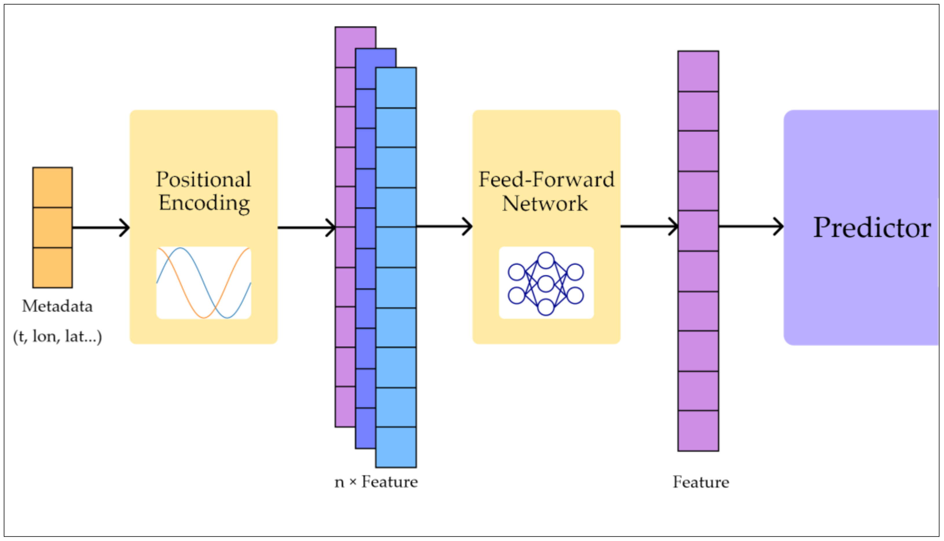
Figure 3 illustrates the architecture of the Metadata Embedding module. The module includes a positional encoding module and a Feed-Forward Network with a GELU [30] activation function. We utilized sinusoidal positional encoding [31] for the initial encoding of the metadata. Sinusoidal positional encoding provides a unique representation for each position. It captures relative positional relationships through the periodicity of sine and cosine functions. Despite introducing redundancy, sinusoidal positional encoding is a simple and effective positional encoding method due to its multi-scale representation, good generalization ability, and computational efficiency. Each element $E_j$ of the input vector is first encoded into a $d$ sized vector using the following positional encoding formula:

$$PE(E_j,2i)=sin\left(\frac{E_j}{{10000}^{2i/d}}\right)$$

$$PE(E_j,2i+1)=cos\left(\frac{E_j}{{10000}^{2i/d}}\right)$$

Then, through two layers of fully connected networks, a metadata feature of size $d$ is obtained. The hyperparameter $d$ is the size of the feature output, and it is set to 64 in our model.

This module enables the model to learn the patterns of SSH changes in different regions or at different times, thereby improving the accuracy of SSH prediction.

4.2.3. Predictor

The Predictor module is responsible for predicting the sea features for future time steps based on the features extracted by the Encoder. It employs a ConvNeXt [32] block-based spatial–temporal prediction network that performs causal convolution along the temporal dimension to model the temporal evolution of ocean dynamics. ConvNeXt is a novel convolutional neural network architecture designed for computer vision tasks. ConvNeXt employs a unique design that combines the strengths of convolutional neural networks and transformer models, leveraging the inductive biases of both architectures. Each ConvNeXt block in the Predictor includes components such as depthwise separable convolutions, Layer Normalization, and MLP, effectively capturing the nonlinear dynamic features of ocean dynamics. Through gradual transformations and updates of the feature maps, the Predictor generates high-quality predictions of future sea surface heights.

Moreover, the Predictor incorporates metadata features as additional input. It contains prior information such as relative time, latitude, and longitude, enabling the model to better understand the spatial and temporal patterns in ocean data. As a result, the Predictor can more accurately capture the evolution trends of ocean dynamic processes and generate future ocean features.

Overall, by introducing metadata embedding and adopting a powerful spatio-temporal convolutional network, Predictor can effectively model the long-term evolution patterns of ocean dynamic processes, generating accurate future ocean features. These features contain abundant semantic information about the ocean, which can be restored in the decoder as future sea surface heights and are also applicable to other prediction tasks.

4.2.4. Decoder

The Decoder module is responsible for progressively upsampling and decoding the low-resolution prediction feature maps generated by the Predictor, restoring sea surface height predictions with the same size as the input. It employs a series of transposed convolutional layers to gradually increase the resolution of the feature maps and fuses them with shallow features extracted by the Encoder to recover more refined prediction details.

During the decoding process, the Decoder needs to combine feature information at different scales to generate high-quality prediction results. By incorporating shallow features extracted by the Encoder, the Decoder can fuse high and low-frequency information, preserving global structural consistency while restoring prediction details. This design of skip connections has been widely validated in tasks such as image segmentation and super-resolution, effectively enhancing the visual quality of the generated results.

Finally, the output of the Decoder is mapped through a 1 × 1 convolutional layer to obtain sea surface height prediction results with the same size as the input. By calculating Mean Squared Error (MSE) Loss using actual future time-steps for sea surface height and updating model parameters through backpropagation, this training approach allows for the end-to-end training of the prediction model. As a result, accurate sea surface height predictions with visual similarity to actual sea surface height maps can be achieved.

In summary, the Decoder module employs a transposed convolution-based architecture with large kernel attention (LKA) [33] mechanisms to effectively restore low-resolution prediction feature maps into high-quality sea surface height prediction results. Through strategies such as skip connections and dynamic weight adjustments, the Decoder enhances the spatio-temporal consistency and detail representation of the prediction results, providing reliable support for ocean prediction tasks.

4.2.5. Model Details

Table 1. The detailed breakdown of the model we used. M represents the number of metadata items.

Layer	Sub-Layer	Input Name (Shape)	Output Name (Shape)
Encoder	Conv–LayerNorm–SiLU	InputSeqs: (10,3,64,64)	Enc1: (10,128,64,64)
	(Conv–LayerNorm–SiLU) × 3	Enc1	Enc2: (10,128,16,16)
Metadata Embedding	SinusoidalPosEmb	Metadata: (M)	Metadata: (M × 64)
	Linear	Metadata	Metadata: (256)
	GELU	Metadata	Metadata: (256)
	Linear	Metadata	Metadata: (64)
Predictor	Concat + Reshape	Learnable Parameter: (10,128,16,16), Enc2	Pred: (2560,16,16)
	ConvNeXt bottle	Pred	Pred: (1280,16,16)
	Linear	Metadata	Metadata_emb: (128)
	Add	Pred, Metadata_emb	Pred: (1280,16,16)
	ConvNeXt bottle	Pred	Pred: (1280,16,16)
	Linear	Metadata	Metadata_emb: (128)
	Add	Pred, Metadata_emb	Pred: (1280,16,16)
	ConvNeXt bottle	Pred	Pred: (1280,16,16)
	Linear	Metadata	Metadata_emb: (128)
	Add	Pred, Metadata_emb	Pred: (1280,16,16)
	Linear	Metadata	Metadata_emb: (128)
	ConvNeXt bottle	Pred	Pred: (1280,16,16)
	Linear	Metadata	Metadata_emb: (128)
	Add	Pred, Metadata_emb	Pred: (1280,16,16)
	ConvNeXt bottle	Pred	Pred: (1280,16,16)
	Linear	Metadata	Metadata_emb: (128)
	Add	Pred, Metadata_emb	Pred: (1280,16,16)
	Reshape	Pred	Pred: (10,128,16,16)
Decoder	TransposedConv-LayerNorm-SiLU	Pred	Dec: (10,128,16,16)
	TransposedConv-LayerNorm-SiLU	Dec	Dec: (10,128,32,32)
	TransposedConv-LayerNorm-SiLU	Dec	Dec: (10,128,64,64)
	Add	Dec, Enc1	Dec: (10,256,64,64)
	TransposedConv-LayerNorm-SiLU	Dec	Dec: (10,128,64,64)
	Reshape	Dec	Dec: (1280,64,64)
	2D 1 × 1 Convolution	Dec	Dec: (64,64,64)
	Large Kernel Attention (LKA)	Dec	Dec: (64,64,64)
	2D 1 × 1 Convolution	Dec	Output: (1,64,64)

, below, shows the precise model architecture, outlining layer specifics for each component along with input and output tensor shapes, which can be used for replicating the model.

4.3. Eddy Detection Algorithm

The main purpose of the eddy detection algorithm is to automatically identify and track eddy structures in ocean currents for a better understanding of ocean dynamic processes. This algorithm requires processing a large amount of ocean data, typically including sea surface height, geostrophic current, and sea surface temperature.

Table 2. The comparison of various mesoscale eddy detection algorithms.

Method	Category	Principle	Features
Okubo–Weiss	Physical parameter-based	Uses the Okubo–Weiss parameter to determine eddy cores based on coherent regions of negative W for both cyclonic and anticyclonic eddies.	Low excessive detection rate (EDR). Low successful detection rate (SDR). Moderate definition of eddy boundary (radius).
Vector–Geometry	Flow geometry-based	Uses geometric characteristics of the velocity field to identify eddies, requiring velocity vectors in adjacent quadrants inside a chosen area to successively change by roughly the same angle and rotate constantly with same (anticyclonic) or opposite (cyclonic) sign.	Sensitive to data resolution. Good detection of weak eddies when using high resolution data.
Winding Angle	Flow geometry-based	Uses a certain SLA value and swirling vectors to determine eddy boundary; computes the winding angle and clusters particles released in the geostrophic current field into anticyclonic (cyclonic) eddies.	High SDR. Tends to detect eddies with larger boundaries.
Angular Momentum Eddy Detection and Tracking Algorithm (AMEDA) [35]	Hybrid (physical parameter + flow geometry)	Uses local normalized angular momentum (LNAM) to detect eddy centers and closed streamlines to determine eddy boundary; can track eddy merging and splitting events.	Robust to grid resolution. Uses a minimal number of tunable parameters. Quantifies dynamical eddy features.

presents common algorithms for detecting mesoscale eddies and their characteristics, each with their own advantages, disadvantages, and conditions of applicability [34].

In our work, we utilized the AMEDA algorithm as the eddy detection module in the eddy prediction framework. The Angular Momentum Eddy Detection and Tracking Algorithm (AMEDA) combines angular momentum and geometric features for eddy detection. It first determines the eddy centers on each grid point based on local angular momentum and constructs closed contour lines. Then, the algorithm calculates the radius and velocity of each closed contour line, detecting any merging or splitting events. Finally, it tracks and analyzes the evolution and interactions of eddies at each time step. The algorithm ultimately provides detailed information on all eddies within the detection area. This information includes the eddy center (a single coordinate), the eddy outline (a set of points enclosing the eddy region), and the eddy properties (either cyclonic or anticyclonic). We utilized the eddy outline for visualizing predicted eddies and measured the effectiveness of eddy predictions by calculating the distance between the predicted eddy center and the true value.

5. Experiments

5.1. Setup

The model training and prediction were performed using the following computer hardware and software configuration: NVIDIA RTX 4090 graphics card; Intel(R) Core (TM) i7-13700F CPU; 64 GB RAM; Windows 11 22H2 operating system; Python 3.10.13 interpreter; NumPy 1.26.0; PyTorch 2.1.0. We used the AdamW [36] Optimizer with parameters ${(learning\_rate=0.0005, \beta }_1=0.9, { \beta }_2=0.999, \lambda =0.01)$ and Mean Square Loss (MSE) loss function for our model training. Due to limited memory, the batch size for training was set at 10.

5.2. Metrics

5.2.1. Root Mean Square Error (RMSE)

Root Mean Square Error (RMSE) is a measure of the accuracy of the SSH prediction model. It indicates the average deviation between the predicted values and the true values, the smaller the better. The formula for RMSE is as follows:

$$RMSE=\sqrt{\frac{1}{n}\sum _{i=1}^n {\left(y_i-{\widehat{y}}_i\right)}^2}$$

where $n$ is the number of samples, $y_i$ is the true value of the i-th sample, and ${\widehat{y}}_i$ is the predicted value of the i-th sample.

5.2.2. Mean Absolute Error (MAE)

Mean Absolute Error (MAE) is a metric used to evaluate the performance of the SSH prediction model. It is defined as the average absolute difference between the predicted values of the model and the true values of the data. The MAE is calculated using the following formula:

$$MAE=\frac{1}{n}\sum _{i=1}^n |y_i-{\widehat{y}}_i|$$

where $n$ is the number of observations in the data, $y_i$ is the true value of the i-th observation, and ${\widehat{y}}_i$ is the predicted value of the i-th observation.

5.2.3. Average Center Distance and Match Rate

The main indicators used to evaluate the effectiveness of mesoscale eddy prediction in our study were the average center distance and the match rate. For a predicted sea surface height image ${\widehat{y}}_i$ and the corresponding ground truth image $y_i$, we first applied an eddy detection algorithm $D$ to obtain the set of center points of mesoscale eddies on the sea surface height images, denoted as $c=D\left(y_i\right)$ and $\widehat{c}=D\left({\widehat{y}}_i \right)$. Subsequently, we constructed a bipartite graph using $V=\{c,\widehat{c}\}$ as the vertex set, with the edge weight being the absolute distance between the eddy center points, to perform a minimum weight matching to obtain the set of matched points. This process allowed us to calculate the Average Center Distance as follows:

$$AvgDis=\frac{\sum _{i=1}^n di{s}_i}{n}$$

The variable $di{s}_i$ represents the weight of the i-th edge of matching, representing the distance between the predicted eddy center and the actual value, measured in kilometers. $n$ denotes the total number of matched points.

The Match Rate indicates the frequency at which the eddy centers in the actual values are successfully matched. It can be calculated by the following formula:

$$MatchRate=\frac{n}{N}$$

The variable $N$ denotes the total number of ground truth eddy center points.

5.3. Sea Surface Height (SSH) Prediction Results

In this section, we employed large-scale ADT prediction and single-window SLA prediction methods to assess the performance variations of our different models across various time intervals and datasets. Large-area prediction involves the use of a sliding window to sample the dataset within a large area, allowing for predictions of sea surface heights at any window position within the area. On the other hand, single-window area prediction focuses only on a fixed small area, aiming to achieve better results than large-area prediction. The large-area predictive model saves computational resources significantly, while the single-window predictive model provides a significant improvement in effectiveness compared to the large-area predictive model.

5.3.1. Large Area ADT Prediction Results

In this section, we utilize the ADT and UGOS, VGOS data from the “Global Ocean Gridded L4 Sea Surface Heights And Derived Variables Nrt” product to train models for predicting future ADT data in a large region. The study area was defined by the region bounded by 107.875°E to 179.875°E in longitude and 39.875°N to 39.875°S in latitude. Due to the larger size of the target region for training and prediction compared to the input–output area of the model, we employed a sliding window approach to extract data of the same size as the model’s input and output from the larger dataset. We then gathered the metadata proposed in Section 4.2.2 to form the dataset. The training and validation data were from the years 2019 to 2020, while the testing data were from 2021. We selected 11 consecutive time steps with a time interval of 3 days between each time step, setting the window size to be $64\times 64$ pixels, corresponding to the spatial resolution of the data product. Each pixel represented a $0.25°\times 0.25°$ grid cell on the Earth surface. The window was moved in both longitude and latitude directions with a stride of 24 pixels.

In 3-day prediction, the input data’s time series were derived from the remote sensing image frames of the past 28 days, with 10 frames sampled as input at 3-day intervals. In 7-day prediction, we used a specific time interval sequence of past SSH frames to help the model better capture the long-term and short-term changes in the ocean. In brief, the input consisted of 10 frames with relative days of i, i + 7, i + 14, i + 17, i + 20, i + 23, i + 26, i + 27, i + 28, and i + 29, while the predicted frame, or label, corresponded to day i + 36. We trained these models for 100 epochs.

We divided the experiment into four groups: the first group trained using ADT and UGOS, VGOS channels with the Metadata Embedding module (3dim-ME), the second group trained using ADT and UGOS, VGOS channels without the Metadata Embedding module (3dim), the third group trained using only the ADT channel with the Metadata Embedding module (1dim-ME), and the fourth group trained using only velocity channels with the Metadata Embedding module (UV-ME). We also employed a ConvLSTM [37] with 5 hidden layers and a hidden dimension of 64 for comparison.

Table 3. Large area ADT prediction experiment results and performance comparison.

Timestep	Model	Test Loss
		RMSE (m)	MAE (m)
3 days	IAM4VP-3dim-ME	0.0108	0.0084
	IAM4VP-3dim	0.0110	0.0085
	IAM4VP-1dim-ME IAM4VP-UV-ME	0.0111 0.0476	0.0087 0.0381
	ConvLSTM	0.0541	0.0425
7 days	IAM4VP-3dim-ME	0.0216	0.0167
	IAM4VP-3dim	0.0221	0.0172
	IAM4VP-1dim-ME	0.0228	0.0177
	IAM4VP-UV-ME	0.0515	0.0380
	ConvLSTM	0.0564	0.0440

shows the performances of these models. The model performed best when using velocity input combined with Metadata Embedding. It obtained an RMSE of 0.0108 m and MAE of 0.0084 m for 3-day prediction, and an RMSE of 0.0216 m and MAE of 0.0167 m for 7-day prediction. The model’s performance using only ADT as input with Metadata Embedding was second-best, achieving an RMSE of 0.0110 m and MAE of 0.0085 m for the 3-day prediction and an RMSE of 0.0221 m and MAE of 0.0172 m for the 7-day prediction. The model performed less well when using velocity input without Metadata Embedding, achieving RMSE and MAE values of 0.0111 m and 0.0087 m for the 3-day prediction, and 0.0228 m and 0.0177 m for the 7-day prediction. When using only velocity input along with metadata embedding, the model attained an RMSE of 0.0476 m and an MAE of 0.0381 m for 3-day prediction. As for 7-day prediction, the RMSE and MAE values were 0.0515 m and 0.0380 m, respectively. ConvLSTM exhibited poorer performance, achieving RMSE and MAE values of 0.0541 m and 0.0425 m for the 3-day prediction and 0.0564 m and 0.0440 m for the 7-day prediction. Figure 4 shows the error distribution of our model on the test dataset. It can be observed that the absolute error in the 3-day prediction was almost always within 0.05 m, while the performance in the 7-day prediction was noticeably worse. Overall, the prediction performance of 7-day prediction was significantly inferior to 3-day prediction.

When the model is trained and used to make predictions based on data from a large area, the varying locations of data sources significantly impact the accuracy of the model’s predictions. In other words, the difficulty of predicting data varies across different locations. Figure 5 illustrates the distribution of RMSE in predicting the model at different locations within the area we studied for 3-day and 7-day prediction. There are many parts in the image without points due to missing data in the dataset, mainly caused by missing data in land areas. It can be observed from the figure that the model seems to perform worse near the missing values and better and more consistently in areas without missing values.

5.3.2. Single-Window Area SLA Prediction Results

In this section, we used single-window-size area data from the “Global Ocean Gridded L4 Sea Surface Heights and Derived Variables Reprocessed 1993 Ongoing” product to predict the sea level anomaly (SLA) 3 or 7 days later. Training in a single-window-size area means that only the sea surface height within that particular window can be predicted, but it is apparent that higher accuracy can be achieved. Multiple models can be trained using this method to predict sea surface height in larger areas. Since the prediction location is static, the Metadata Embedding module only provides relative time information $t$ proposed in Section 4.2.2, as the location metadata is static.

We conducted tests on data from three different regions. Our training data were sourced from the region with the specified latitude and longitude (Region 1, 13.375°N~29.125°N, 139.375°E~123.125°E) and two areas in Kuroshio Extension (Region 2, 26.125°N~41.875°N, 179.875°E~163.625°E; Region 3, 26.125°N~41.875°N, 167.875°E~151.625°E) as our research sample to predict mesoscale eddies. Due to the lower accuracy of edge areas in the predicted numerical image compared to the center areas [4], we only selected the central 50 × 50 region of the numerical image for output to calculate the loss and assess the accuracy. The training and validation data were from the years 1993 to 2017, while the testing data span from 2018 to 2021. To the best of our knowledge, our model performed the best among all known methods for this specific task.

First, we trained a 7-day prediction for Region 1 for 100 epochs. Region 1 was chosen to compare performance with Enhanced MIM [19] for SLA prediction.

Table 4. Comparison of the model performance in Region 1 prediction. Models were trained and tested using the same data source, same region, and similar timestep.

Model (Timestep)	Test Loss
	RMSE (m)	MAE (m)
IAM4VP-ME (7 days)	0.0110	0.0083
Enhanced MIM (6 days)	0.017	/
Enhanced MIM (8 days)	0.019	/

shows the performances of these models. Even though the Enhanced MIM paper did not include a 7-day prediction experiment, our 7-day prediction in this area resulted in an RMSE of 0.0110 m and MAE of 0.0083 m, significantly outperforming their 6-day prediction with an RMSE of 0.017 m.

Then, we used the weights of this model as pre-training weights for training models in Regions 2 and 3. Using the pre-training weights, only 5 to 10 epochs of fine-tuning are needed to achieve good results, as higher numbers of epochs can lead to severe overfitting.

Table 5. Comparison of the model performance in two different time intervals within the Kuroshio Extension area.

Timestep	Test Loss
	Region 2		Region 3
	RMSE (m)	MAE (m)	RMSE (m)	MAE (m)
3 days	0.0033	0.0025	0.0030	0.0023
7 days	0.0097	0.0076	0.0087	0.0061

shows the performance of our single-window-size SSH prediction model. The results indicate that the RMSE values for the 3-day prediction in two regions were 0.0033 m and 0.0030 m, with corresponding MAE values of 0.0025 m and 0.0023 m. For the 7-day prediction in two regions, the RMSE values were 0.0097 m and 0.0087 m, with MAE values of 0.0076 m and 0.0061 m. Figure 6 and Figure 7 display the performance of 3-day and 7-day predictions. The results demonstrate that employing single-window area prediction significantly enhances prediction accuracy, with considerable differences in accuracy observed across different regions.

In addition, the spatial distribution of errors in the 3-day prediction is relatively uniform, while in the 7-day prediction, the spatial distribution of errors is more uneven. Figure 8 depicts the distribution of errors for 3-day and 7-day prediction. The results indicate that the error for the 3-day predictions was nearly always below 0.01 m, whereas the accuracy of the 7-day prediction was slightly lower.

5.4. Mesoscale Eddy Prediction Results

In this section, we tested and evaluated the predictions of mesoscale eddies in the Kuroshio Extension region. We utilized the model from Section 4.2 to predict the sea level anomaly (SLA) gridded data for the Kuroshio Extension region for the period from 8 February 2022 to 31 July 2022. The test areas were as follows: (Area 1: 27.875°N~40.125°N, 166.125°E~153.875°E) and (Area 2: 27.875°N~40.125°N, 178.125°E~165.875°E), corresponding to the Region 2 and 3 cropping of a 50 × 50 center area mentioned in Section 5.3.2. We applied the AMEDA algorithm to detect mesoscale eddies in both predicted and ground truth sea level anomaly (SLA) series and compared the results from both sets of eddy detections. The performance evaluation will focus on the deviation of the eddy center and the prediction of the mesoscale eddies’ lifespan. Figure 9 shows examples of eddy detection results with SLA maps. The result demonstrates that our method accurately predicts larger mesoscale eddies, but may inaccurately predict or fail to predict the location of some smaller mesoscale eddies.

First, we conducted a statistical analysis of the total detection counts for cyclonic and anticyclonic eddies. Figure 10 shows the total counts of cyclonic and anticyclonic eddies for different datasets. We found that the original dataset had the highest detection capabilities for eddies, followed by the 3-day prediction and the 7-day prediction, which detected fewer eddies. We found that this method performs less well for smaller eddies, primarily due to the lag in predicting the appearance of eddies and the tendency to anticipate the disappearance of eddies.

We matched the actual and predicted positions of the eddy centers at the same time and location to evaluate the performance of the eddy prediction. To address the problem of aligning predicted and actual eddy center positions, we transformed the sets of predicted and actual eddy centers for each day into a bipartite graph. We then determined the minimum-weight matching by considering the actual distances between the points. During the construction of the bipartite graph, edges with real distances (edge weights) exceeding 100 km are ignored due to the significant deviation of eddy centers, which may likely not represent a correct match.

Table 6. Assessment of mesoscale eddy predictions with different time steps in two regions.

Prediction Area/Time Step	Average Center Distance (km)	Match Rate
Area 1, 3-day	4.5566	94.02%
Area 1, 7-day	11.6794	86.57%
Area 2, 3-day	6.6462	92.48%
Area 2, 7-day	15.5567	82.28%

presents the results of the evaluation of eddy prediction after matching. In the 3-day prediction, Area 1 achieved an Average Center Distance of 4.5566 km and a Match Rate of 94.02%, while Area 2 had an Average Center Distance of 6.6462 km and a Match Rate of 92.48%. In the 7-day prediction, Area 1 achieved an Average Center Distance of 11.6794 km and a Match Rate of 86.57%, while Area 2 had an Average Center Distance of 15.5567 km and a Match Rate of 82.28%. As the prediction time increases, the difficulty of prediction also rises, resulting in lower accuracy of the predicted eddy. The decrease in match rate is associated with lagging predictions of eddy appearance and a loss of image details, leading to undetectable eddies.

Figure 11 illustrates the distribution of distances between the predicted eddy centers and the actual values. We found that predicting mesoscale eddies using the 3-day prediction of sea surface height has very high accuracy. Most of the predicted eddy centers deviated from the true values by less than 20 km. However, the accuracy slightly decreased in the 7-day prediction, and the match rate also declined. Combining with the results in Figure 9, this may be attributed to the higher difficulty in predicting sea surface height, leading to inaccuracies in the reflected eddy information in the predicted SSH data.

Table 7. The comparison of various mesoscale eddy prediction methods and our proposed method.

Method	Dataset	Data Range	Average Center Offset Distance (Prediction Time)	Prediction of the Generation and Disappearance
Multiple Linear Regression [16]	AVISO (L4 SSH, Eddy Trajectory dataset) GDEM V3 (Ocean Temperature, Salinity)	Northern South China Sea	36.9 km (anticyclonic), 41.1 km (cyclonic) (7 days) 81.0 km (anticyclonic), 88.5 km (cyclonic) (14 days)	×
LSTM + ET [18]	AVISO (Eddy Trajectory dataset)	South China Sea (5°~25°N, 105°~125°E)	10.6 km (1 day) 23.3 km (7 days)	×
Enhanced MIM [19]	AVISO (L4 SSH)	Western Pacific Ocean (125°~137.5°E, 15°~27.5°N)	21.43 km (7 days) 29.8 km (14 days)	√
MesoGRU [20]	AVISO (Eddy Trajectory dataset) CMEMS (L4 SSH)	South China Sea (4°~21°N, 105°~118°E)	8 km (1 day) 18.5 km (14 days)	×
IAM4VP with ME (Ours)	CMEMS (L4 SSH)	Kuroshio Extension (27.875°N~40.125°N, 166.125°E~153.875°E) and (27.875°N~40.125°N, 178.125°E~165.875°E)	5.6267 km (3 days) 13.6315 km (7 days)	√

presents a comparison of various mesoscale eddy prediction methods, including our proposed IAM4VP with ME approach. The methods are evaluated based on the datasets used, the geographical data range, the average center offset distance at different time offsets, and their ability to predict the generation and disappearance of mesoscale eddies.

Among the compared methods, our IAM4VP with ME approach demonstrated superior performance in terms of the average center offset distance, achieving 5.6267 km at a 3-day time offset and 13.6315 km at a 7-day time offset. Furthermore, our method was capable of predicting both the generation and disappearance of mesoscale eddies, a feature that is only shared by the Enhanced MIM method. The other methods, such as LSTM and ET and MesoGRU, do not provide this capability. In conclusion, our IAM4VP with ME approach exhibited high performance in mesoscale eddy prediction, offering accurate predictions of eddy center positions and the ability to forecast the generation and disappearance of eddies.

6. Conclusions

In our study, we employed a deep learning SSH prediction model to predict sea surface height. Then, we utilized the predicted sea surface height data for eddy detection to predict mesoscale eddies. For the sea surface height prediction, we incorporated ADT and SLA data from CMEMS, and integrated geostrophic velocity data as the training dataset. We constructed a sea surface height prediction model based on the deep learning model IAM4VP and incorporated a Metadata Embedding module to enable the model to learn the patterns of sea surface height variations in different regions and times. The experimental results demonstrated that the fusion of velocity data and the Metadata Embedding module enhanced the performance of the sea surface height prediction model. Furthermore, in addition to training the model with large-area sea surface height data, we also explored the use of a fixed small area for single-window area SSH prediction. This approach allowed the model to focus on prior knowledge within the same geographical location and predict the sea surface height exclusively within that small region, significantly improving prediction accuracy. Our model obtained RMSE values of 0.0033 m and 0.0030 m, as well as MAE values of 0.0025 m and 0.0023 m, respectively, in two chosen regions for 3-day prediction. For the 7-day prediction in two regions, we achieved RMSE 0.0097 m and 0.0087 m, with MAE 0.0076 m and 0.0061 m. The empirical results validated that our model outperformed the best-known models of the same type. Lastly, we employed the AMEDA algorithm to perform eddy detection on the predicted sea surface height data and thus obtained the prediction results for mesoscale eddies. We analyzed the errors in the 3-day and 7-day prediction results in comparison to the ground truth values. The results indicate that both the 3-day and 7-day predictions have high accuracy. In the 3-day prediction in two selected areas, the average distance of the eddy center deviation reached 4.5566 km and 6.6462 km, while in the 7-day prediction, it reached 11.6794 km and 15.5567 km.

References

- Siegel, D.A.; Granata, T.C.; Michaels, A.F.; Dickey, T.D. Mesoscale eddy diffusion, particle sinking, and the interpretation of sediment trap data. J. Geophys. Res. Oceans 1990, 95, 5305–5311. [Google Scholar] [CrossRef]
- Chelton, D.B.; Schlax, M.G.; Samelson, R.M.; de Szoeke, R.A. Global observations of large oceanic eddies. Geophys. Res. Lett. 2007, 34, L15606. [Google Scholar] [CrossRef]
- Wyrtki, K.; Magaard, L.; Hager, J. Eddy energy in the oceans. J. Geophys. Res. 1976, 81, 2641–2646. [Google Scholar] [CrossRef]
- Fu, L.; Chelton, D.; Traon, P.L.; Morrow, R.A. Eddy dynamics from satellite altimetry. Oceanography 2010, 23, 14–25. [Google Scholar] [CrossRef]
- Yang, G.; Wang, F.; Li, Y.; Lin, P. Mesoscale eddies in the northwestern subtropical Pacific Ocean: Statistical characteristics and three-dimensional structures. J. Geophys. Res. Oceans 2013, 118, 1906–1925. [Google Scholar] [CrossRef]
- Mason, E.; Pascual, A.; McWilliams, J.C. A new sea surface height–based code for oceanic mesoscale eddy tracking. Atmos. Ocean. Technol. 2014, 31, 1181–1188. [Google Scholar] [CrossRef]
- Robinson, A.R.; Carton, J.A.; Mooers, C.N.K.; Walstad, L.J.; Carter, E.F.; Rienecker, M.M.; Smith, J.A.; Leslie, W.G. A real-time dynamical forecast of ocean synoptic/mesoscale eddies. Nature 1984, 309, 781–783. [Google Scholar] [CrossRef]
- Robinson, A.R.; Leslie, W.G. Estimation and prediction of oceanic eddy fields. Prog. Oceanogr. 1985, 14, 485–510. [Google Scholar] [CrossRef]
- Rienecker, M.M.; Mooers, C.N.K.; Robinson, A.R. Dynamical interpolation and forecast of the evolution of mesoscale features off northern California. J. Phys. Oceanogr. 1987, 17, 1189–1213. [Google Scholar] [CrossRef]
- Masina, S.; Pinardi, N. Mesoscale data assimilation studies in the Middle Adriatic Sea. Cont. Shelf Res. 1994, 14, 1293–1310. [Google Scholar] [CrossRef]
- Isern-Fontanet, J.; García-Ladona, E.; Font, J. Identification of marine eddies from altimetric maps. J. Atmos. Ocean. Technol. 2003, 20, 772–778. [Google Scholar] [CrossRef]
- Hurlburt, H.E.; Chassignet, E.P.; Cummings, J.A.; Kara, A.B.; Metzger, E.J.; Shriver, J.F.; Smedstad, O.M.; Wallcraft, A.J.; Barron, C.N. Eddy-resolving global ocean prediction. Ocean Model. Eddying Regime Geophys. Monogr. 2008, 177, 353–381. [Google Scholar]
- Prants, S.V.; Budyansky, M.V.; Uleysky, M.Y. Lagrangian simulation and tracking of the mesoscale eddies contaminated by Fukushima-derived radionuclides. Ocean Sci. 2017, 13, 453–463. [Google Scholar] [CrossRef]
- Chassignet, E.P.; Hurlburt, H.E.; Smedstad, O.M.; Halliwell, G.R.; Hogan, P.J.; Wallcraft, A.J.; Bleck, R. Ocean Prediction with the Hybrid Coordinate Ocean Model (HYCOM). In Ocean Weather Forecasting; Chassignet, E.P., Verron, J., Eds.; Springer: Dordrecht, The Netherlands, 2006. [Google Scholar] [CrossRef]
- Fu, Y.; Zhou, X.; Sun, W.; Tang, Q. Hybrid model combining empirical mode decomposition, singular spectrum analysis, and least squares for satellite-derived sea-level anomaly prediction. Int. J. Remote Sens. 2019, 40, 7817–7829. [Google Scholar] [CrossRef]
- Li, J.; Wang, G.; Xue, H.; Wang, H. A simple predictive model for the eddy propagation trajectory in the northern South China Sea. Ocean Sci. 2019, 15, 401–412. [Google Scholar] [CrossRef]
- Ma, C.; Li, S.; Wang, A.; Yang, J.; Chen, G. Altimeter observation-based eddy nowcasting using an improved Conv-LSTM network. Remote Sens. 2019, 11, 783. [Google Scholar] [CrossRef]
- Wang, X.; Wang, H.; Liu, D.; Wang, W. The prediction of oceanic mesoscale eddy properties and propagation trajectories based on machine learning. Water 2020, 12, 2521. [Google Scholar] [CrossRef]
- Nian, R.; Cai, Y.; Zhang, Z.; He, H.; Wu, J.; Yuan, Q.; Geng, X.; Qian, Y.; Yang, H.; He, B. The Identification and Prediction of Mesoscale Eddy Variation via Memory in Memory with Scheduled Sampling for Sea Level Anomaly. Front. Mar. Sci. 2021, 8, 753942. [Google Scholar] [CrossRef]
- Wang, X.; Wang, X.; Yu, M.; Li, C.; Song, D.; Ren, P.; Wu, J. MesoGRU: Deep learning framework for mesoscale eddy trajectory prediction. IEEE Geosci. Remote Sens. Lett. 2021, 19, 8013805. [Google Scholar] [CrossRef]
- Zhu, Y.; Peng, S.; Li, Y. A vortex-implanted initialization scheme for the mesoscale eddy prediction: Idealized experiments. Front. Mar. Sci. 2022, 9, 1009852. [Google Scholar] [CrossRef]
- Scher, S.; Messori, G. Weather and climate forecasting with neural networks: Using general circulation models (GCMs) with different complexity as a study ground. Geosci. Model Dev. 2019, 12, 2797–2809. [Google Scholar] [CrossRef]
- Weyn, J.A.; Durran, D.R.; Caruana, R. Can machines learn to predict weather? Using deep learning to predict gridded 500-hPa geopotential height from historical weather data. J. Adv. Model. Earth Syst. 2019, 11, 2680–2693. [Google Scholar] [CrossRef]
- Weyn, J.A.; Durran, D.R.; Caruana, R.; Cresswell-Clay, N. Sub-seasonal forecasting with a large ensemble of deep-learning weather prediction models. J. Adv. Model. Earth Syst. 2021, 13, e2021MS002502. [Google Scholar] [CrossRef]
- Copernicus Marine Service. Global Ocean Gridded L4 Sea Surface Heights and Derived Variables Nrt. 2023. Available online: https://data.marine.copernicus.eu/product/SEALEVEL_GLO_PHY_L4_NRT_008_046/description (accessed on 7 October 2023).
- Copernicus Marine Service. Global Ocean Gridded L4 Sea Surface Heights and Derived Variables Reprocessed 1993 Ongoing. 2023. Available online: https://data.marine.copernicus.eu/product/SEALEVEL_GLO_PHY_L4_MY_008_047/description (accessed on 7 October 2023).
- Seo, M.; Lee, H.; Kim, D.; Seo, J. Implicit Stacked Autoregressive Model for Video Prediction. arXiv 2023, arXiv:2303.07849. [Google Scholar] [CrossRef]
- Elfwing, S.; Uchibe, E.; Doya, K. Sigmoid-weighted linear units for neural network function approximation in reinforcement learning. Neural Netw. 2018, 107, 3–11. [Google Scholar] [CrossRef] [PubMed]
- Dosovitskiy, A.; Beyer, L.; Kolesnikov, A.; Weissenborn, D.; Zhai, X.; Unterthiner, T.; Dehghani, M.; Minderer, M.; Heigold, G.; Gelly, S.; et al. An Image is Worth 16 × 16 Words: Transformers for Image Recognition at Scale. In Proceedings of the 9th International Conference on Learning Representations (ICLR), Virtual Event, 3–7 May 2021. [Google Scholar]
- Hendrycks, D.; Gimpel, K. Gaussian Error Linear Units (GELUs). arXiv 2016, arXiv:1606.08415. [Google Scholar] [CrossRef]
- Vaswani, A.; Shazeer, N.; Parmar, N.; Uszkoreit, J.; Jones, L.; Gomez, A.N.; Kaiser, Ł.; Polosukhin, I. Attention is all you need. In Proceedings of the 31st International Conference on Neural Information Processing Systems (NIPS), Long Beach, CA, USA, 4–9 December 2017; pp. 6000–6010. [Google Scholar]
- Liu, Z.; Mao, H.; Wu, C.-Y.; Feichtenhofer, C.; Darrell, T.; Xie, S. A ConvNet for the 2020s. In Proceedings of the IEEE/CVF Conference on Computer Vision and Pattern Recognition (CVPR), New Orleans, LA, USA, 18–24 June 2022; pp. 11966–11976. [Google Scholar]
- Guo, M.H.; Lu, C.Z.; Liu, Z.N.; Cheng, M.M.; Hu, S.M. Visual attention network. Comput. Vis. Media 2023, 9, 733–752. [Google Scholar] [CrossRef]
- Xing, T.; Yang, Y. Three Mesoscale Eddy Detection and Tracking Methods: Assessment for the South China Sea. J. Atmos. Ocean. Technol. 2020, 38, 243–258. [Google Scholar] [CrossRef]
- Le Vu, B.; Stegner, A.; Arsouze, T. Angular Momentum Eddy Detection and Tracking Algorithm (AMEDA) and Its Application to Coastal Eddy Formation. J. Atmos. Ocean. Technol. 2018, 35, 739–762. [Google Scholar] [CrossRef]
- Loshchilov, I.; Hutter, F. Decoupled Weight Decay Regularization. In Proceedings of the 6th International Conference on Learning Representations (ICLR), Toulon, France, 24–26 April 2017. [Google Scholar]
- Shi, X.; Chen, Z.; Wang, H.; Yeung, D.-Y.; Wong, W.-K.; Woo, W.-C. Convolutional LSTM Network: A machine learning approach for precipitation nowcasting. In Proceedings of the 28th International Conference on Neural Information Processing Systems (NIPS), Montreal, QC, Canada, 7–12 December 2015; pp. 802–810. [Google Scholar]
Figure 1.
The architecture of our eddy prediction method. In the SSH prediction component, a deep learning model consisting of an Encoder, Metadata Embedding Module, Predictor, and Decoder takes a sequence of sea surface height and velocity along with its metadata as the input to predict the sea surface height several days later, utilizing MSE Loss for training. In the mesoscale eddy prediction component, the trained SSH prediction model is employed to predict sea surface height, which is then used for detecting mesoscale eddies, thus obtaining the prediction results for mesoscale eddies.
Figure 2.
The architecture of our SSH prediction model. This convolution-based deep learning model consists of an Encoder, Metadata Embedding Module, Predictor, and Decoder, using sea surface height and velocity data as the input. Section 4.2.5 provides a detailed overview of the model’s composition.
Figure 3.
A simplified image representation of the Metadata Embedding Module.
Figure 4.
The error distribution in the large area ADT predictions. Each graph shows the absolute error (m) on the horizontal axis and the frequency on the vertical axis. The first and second images show the results for predictions over 3 days and 7 days, respectively.
Figure 5.
The distribution of RMSE across different regions. The points on the graph represent the central coordinates of a data point. The axes represent longitude and latitude in degrees, with western longitude and northern latitude specified as positive directions.
Figure 6.
A sample of single-window area 3-day prediction results. The columns from left to right show the predicted image, the ground truth image, the error, and the scatter plot with the fitted line of predicted value versus true value. The error is the result obtained by calculating the difference between the predicted image and the ground truth image. The color bar and scatter plot measurements are in meters.
Figure 7.
A sample of single-window area 7-day prediction results. The columns from left to right show the predicted image, the ground truth image, the error, and the scatter plot with the fitted line of predicted value versus true value. The error is the result obtained by calculating the difference between the predicted image and the ground truth image. The color bar and scatter plot measurements are in meters.
Figure 8.
The error distribution in the single-window area SLA predictions. Each graph shows the absolute error (m) on the horizontal axis and the frequency on the vertical axis. The first and second columns represent the results of Region 2 and Region 3 in the test data, while the first and second rows show the results for predictions over 3 days and 7 days, respectively.
Figure 9.
Examples of eddy detection results with SLA maps. The white circles represent the shape of the eddies, with the points inside the circles indicating the position of the eddy centers. This shape and center position information is calculated by the eddy detection algorithm.
Figure 10.
Total detection count of cyclonic/anticyclonic eddies in Area 1 and Area 2.
Figure 11.
Distributions of eddy center distances at different time steps in different regions.