
Impacts of the Sudden Stratospheric Warming on Equatorial Plasma Bubbles: Suppression of EPBs and Quasi-6-Day Oscillations


1
Haystack Observatory, Massachusetts Institute of Technology, Westford, MA 01886, USA
2
High Altitude Observatory, NSF National Center for Atmospheric Research, Boulder, CO 80301, USA
3
ITM Physics Laboratory, Heliophysics Division, NASA Goddard Space Flight Center, Greenbelt, MD 20771, USA
*
Author to whom correspondence should be addressed.
Remote Sens. 2024, 16(8), 1469; https://doi.org/10.3390/rs16081469
Submission received: 28 February 2024
/
Revised: 31 March 2024
/
Accepted: 19 April 2024
/
Published: 21 April 2024
(This article belongs to the Special Issue Advances in Near-Earth Space and Atmospheric Physics from Ground-Based and Satellite Observations)
Abstract
:This study investigates the day-to-day variability of equatorial plasma bubbles (EPBs) over the Atlantic–American region and their connections to atmospheric planetary waves during the sudden stratospheric warming (SSW) event of 2021. The investigation is conducted on the basis of the GOLD (Global Observations of the Limb and Disk) observations, the ICON (Ionospheric Connection Explorer) neutral wind dataset, ionosonde measurements, and simulations from the WACCM-X (Whole Atmosphere Community Climate Model with thermosphere–ionosphere eXtension). We found that the intensity of EPBs was notably reduced by 35% during the SSW compared with the non-SSW period. Furthermore, GOLD observations and ionosonde data show that significant quasi-6-day oscillation (Q6DO) was observed in both the intensity of EPBs and the localized growth rate of Rayleigh–Taylor (R-T) instability during the 2021 SSW event. The analysis of WACCM-X simulations and ICON neutral winds reveals that the Q6DO pattern coincided with an amplification of the quasi-6-day wave (Q6DW) in WACCM-X simulations and noticeable ∼6-day periodicity in ICON zonal winds. The combination of these multi-instrument observations and numerical simulations demonstrates that certain planetary waves like the Q6DW can significantly influence the day-to-day variability of EPBs, especially during the SSW period, through modulating the strength of prereversal enhancement and the growth rate of R-T instability via the wind-driven dynamo. These findings provide novel insights into the connection between atmospheric planetary waves and ionospheric EPBs.
1. Introduction
A significant portion of the ionospheric variability can be driven by lower atmospheric forcing via vertical coupling processes [1,2]. Sudden stratospheric warming (SSW) is one of the most dramatic meteorological events of vertical coupling that occurs in the winter polar stratosphere, driven by the growth and dissipation of upward-propagating planetary waves from the troposphere, as well as their nonlinear interaction with the zonal mean flow [3]. SSW is characterized by a sudden rise in high-latitude stratospheric temperatures by several tens of Kelvin within merely a few days, a displacement or breakdown of the polar vortex, and the weakening (minor warming) or even reversal (major warming) of the zonal-mean zonal wind at the location of 60° latitude and 10 hPa (∼30 km) [4]. Numerous studies have indicated that SSW can not only change the chemistry and dynamics of the stratosphere and mesosphere but also influence the whole atmosphere by adjusting the dynamics, composition, and electrodynamics of the coupled thermosphere–ionosphere system [5,6]. SSW-related wind and temperature changes can alter the amplitudes and phases of tidal waves, which is particularly pronounced in causing the amplification of the lunar semidiurnal tide through resonance, attributed to the atmospheric Pekeris mode, and the solar semidiurnal tide, influenced by the interaction with stationary planetary waves [7,8]. The enhanced tidal perturbations can propagate into the altitudes of the ionospheric E-region and modulate the electric fields through the ionospheric wind dynamo, leading to changes in the E × B plasma drifts and subsequent electron density variation in the ionospheric F-region [9]. Thus, significant variability with diverse temporal scales is observed in the global ionosphere during the SSW period, particularly the enhanced semidiurnal variations over the low-latitude and equatorial regions, such as shown in the vertical plasma drift, e.g., [10,11,12,13,14,15,16], equatorial electrojet, e.g., [17,18,19,20,21], and ionospheric electron density (Ne) and total electron content (TEC), e.g., [5,13,22,23,24,25,26,27,28].
Moreover, notable ionospheric variations during the SSW period with longer temporal scales of multiple days (e.g., ∼2, ∼3, ∼6, ∼10, and ∼16 days) over the low-latitude and equatorial ionosphere have also been extensively documented, e.g., [29,30,31,32,33,34,35]. These multiday oscillations are related to the modulation of planetary waves, including the westward-propagating Rossby waves and the eastward-propagating equatorial Kelvin waves, either through direction propagation into the ionospheric E-region height or via their interactions with and modulation of upward-propagating tides [36,37,38]. Among various planetary waves, the westward-propagating quasi-6-day wave (Q6DW) of the Rossby normal mode, characterized by a zonal wavenumber 1 and a period of 5–8 days, is one of the most prominent and recurrent oscillations within the MLT (mesosphere and lower thermosphere) region, e.g., [39,40,41,42]. Several studies have indicated that the interaction between Q6DW and tides and the subsequent modulation of the equatorial E-region dynamo because of wind disturbances could modify the plasma drift, thereby leading to the generation of quasi-6-day oscillations (Q6DOs) in the ionospheric F-region electron density and TEC over the equatorial ionization anomaly (EIA) regions, e.g., [34,43,44,45,46,47]. Moreover, some studies suggest that the dissipation of planetary waves in the lower thermosphere may induce an additional meridional flow, which could amplify the mixing of thermospheric composition and cause an overall reduction in the thermospheric O/N2 column ratio and ionospheric TEC, e.g., [35,48].
While substantial progress has been achieved in understanding the low-latitude and equatorial ionospheric variation during the SSW period, the potential impact of SSW on equatorial plasma bubbles (EPBs) is an important issue that has not been thoroughly analyzed and explained yet. EPBs refer to irregular ionospheric structures characterized by plasma density depletion with scale sizes ranging from tens to hundreds of kilometers, which usually occur in the equatorial and low-latitude ionosphere after local sunset, spanning from the bottom-side F-region to 1000–2000 km [49,50,51]. EPBs represent some of the most prominent ionospheric plasma disturbances that constitute a noteworthy space weather phenomenon, capable of adversely impacting radio wave propagation and posing severe challenges to navigation systems. Thus, the morphological features and the dynamic evolution of EPBs have been extensively studied using multi-instrument observations and numerical simulations, e.g., [52,53,54,55,56,57,58,59,60,61,62]. It is known that EPBs are generated by the generalized Rayleigh–Taylor (R-T) instability when the bottom-side F-region becomes unstable in the evening with a steep vertical density gradient after the decay of the E-region [63,64,65]. The prereversal enhancement (PRE), characterized by an increase in the eastward electric field and upward plasma drift at the equatorial evening terminator, creates favorable conditions to amplify the growth rate of R-T instability and is considered one of the pivotal factors controlling the development of EPBs [66,67,68]. Although we currently possess a reasonably sound knowledge of the climatological characteristics of EPBS, such as their seasonal and longitudinal variations, e.g., [69,70,71,72,73,74], understanding the complicated day-to-day variability of EPBs and their relationship with lower atmospheric forcing, especially during an SSW, remains a challenging issue for the equatorial space weather community [75,76,77,78].
Some studies have conducted preliminary analyses on the relationship between SSW events and the occurrence rate of equatorial spread-F/scintillation. For example, ref. [79] reported a prolonged weakening of the ionospheric scintillation at a ground-based Global Navigation Satellite System (GNSS) station located in Brazil during three SSW events. Yu et al. [80] and Ye et al. [81] also observed the inhibition of scintillation over the American sector in COSMIC satellite measurements during certain SSW events. Jose et al. [82] presented that the timing of the equatorial spread-F occurrence showed a quasi-16-day oscillation during the SSW years. These studies suggested that the modification of plasma vertical drift during PRE and the altered meridional wind pattern are potential factors causing variations in the equatorial spread-F/scintillation. Moreover, recent pioneering studies have shown that the modulation of tidal winds by planetary waves could have a large impact on the strength of the PRE, thereby leading to planetary-wave-scale oscillations in the intensity of PRE that may potentially influence the day-to-day variability of EPBs [54,83,84,85,86,87]. Nevertheless, there is currently limited observational evidence to demonstrate that signatures of planetary-wave-scale oscillations can be detected in EPBs or the growth rate of R-T instability, and the day-to-day variability of EPBs during SSW deserved a further examination with improved observational and modeling capabilities [86,88].
In the current study, we use multi-instrumental observations and a whole atmospheric model to collectively investigate the day-to-day variation in EPBs during the 2021 SSW, as well as to examine the possible connection between EPBs and planetary waves through the modulation of the R-T instability growth rate. Specifically, the ultraviolet imaging data from the Global-scale Observations of the Limb and Disk (GOLD) is used to characterize the day-to-day variation in EPBs throughout SSW, and equatorial ionosonde data are used to compute the local growth rate of R-T instability as a proxy for EPBs’ occurrence. We found that the intensity of EPBs was notably reduced by 35% during the SSW period compared with the non-SSW period. Moreover, a significant quasi-6-day oscillation (Q6DO) pattern was recorded in both the EPBs and R-T instability growth rate during the SSW. The Ionospheric Connection Explorer (ICON) neutral winds data, combined with simulation results from the Whole Atmosphere Community Climate Model with thermosphere–ionosphere eXtension (WACCM-X), are utilized to analyze the corresponding Q6DW activities in the MLT region and middle atmosphere, respectively. The results show that lower atmospheric waves could play an essential role in controlling the day-to-day variation in EPBs during the SSW period by modulating the strength of the PRE and the growth rate of R-T instability.
2. Observations and Simulations
The GOLD instrument is a UV imaging spectrograph that operates from the geostationary orbit at a longitude of 47.5°W, which observes airglow emissions of Earth within the wavelength range of 134 to 160 nm through the disk, limb, and stellar occultation technique [89,90]. In the evening, the disk measurements of the OI 135.6 nm emission by the GOLD instrument offer continuous and crucial information on the low-latitude and equatorial ionosphere from West Africa to South America, which is particularly valuable for revealing the two-dimensional spatial morphology of EPBs, e.g., [57,88,91,92,93,94]. To characterize the day-to-day variation in EPBs, Aa et al. [88] has developed a new GOLD Bubble Index capable of quantifying the intensity of the bubbles in two dimensions on any given night within the field-of-view of GOLD measurements. In essence, the Bubble Index is computed based on calculating the standard deviation values of the normalized residual radiance at 135.6 nm, which can effectively quantify the short-term (e.g., day-to-day) and long-term (e.g., seasonal and solar cycle) variations in 2D EPBs. To get more information about the GOLD Bubble Index, readers are encouraged to refer to Aa et al. [88]. Moreover, the ionosonde observations from the São Luís station (2.6°S, 44.2°W), located in the equatorial ionosphere, will be used in the study to derive the local growth rate of R-T instability.
The ICON is a low-Earth orbiting satellite that operated within an altitude range of 580–610 km and had an inclination angle of 27° for studying the low-latitude and midlatitude ionosphere and thermosphere [95]. The Michelson interferometer for Global High-resolution Thermospheric Imaging (MIGHTI) is one of the four science instruments of ICON, which can measure the thermospheric wind velocities derived from the Doppler shift of the atomic oxygen emissions at red (630.0 nm) and green (557.7 nm) lines [96]. MIGHTI has two identical sensors to orthogonally measure the horizontal line-of-sight wind at two angles of 45° and 135° relative to the ICON orbit to collectively derive the horizontal wind vector on the northern limb (∼13°) of the orbit. In this study, the ICON-MIGHTI wind data from the green line measurements is utilized to analyze the signatures of planetary waves in the lower thermosphere [97].
WACCM-X is a whole atmosphere community climate model that extends from the surface of Earth to the upper thermosphere (500–700 km), which integrates a thorough treatment of physics, chemistry, electrodynamics, and thermodynamics spanning from the troposphere to the thermosphere–ionosphere [98]. In the current study, to accurately simulate the atmospheric condition during the 2021 SSW event, the WACCM-X simulation uses the specified dynamics to nudge the model toward the meteorological reanalysis data [99], where the lower atmosphere meteorology up to 50 km is constrained to the NASA Modern Era Retrospective Analysis for Research and Applications version-2 (MERRA-2, Gelaro et al. [100]). The F10.7 solar radio flux is utilized to represent the solar irradiance variations, and the Kp index is employed to drive the high-latitude convection and auroral precipitation [101]. This simulation is referred to as LA + S/G (Lower Atmosphere + Solar/Geomagnetic). Besides using the realistic F10.7 and Kp indices, WACCM-X was also run with troposphere–stratosphere being constrained to MERRA-2 but using constant F10.7 (75 solar flux unit) and Kp (0+) values to isolate forcing from the lower atmosphere (LA only). For more content on the WACCM-X simulation, readers could refer to Pedatella et al. [86].
3. Results
Figure 1 depicts the meteorological and solar/geomagnetic activities between December 2020 and March 2021. Figure 1a displays the temporal variation in the stratospheric polar temperature at 60–90°N, 10 hPa (red) and zonal mean zonal wind at 60°N, 10 hPa (blue). The stratospheric polar temperature showed a rapid increase of more than 30 K in just a few days at the beginning of January 2021. The zonal mean zonal wind showed a significant decreasing trend from late December of 2020 and reversed its direction on 5 January 2021. Following the initial reversal, the zonal mean zonal wind remained weak for ∼30 days and experienced two more reversals around days 12–22 and 31–34, associated with small temperature increases. These conditions correspond to a major SSW event, and some early studies have reported enhanced semidiurnal tidal perturbations in the ionosphere [16,26,99,102]. Figure 1b displays the amplitudes of the planetary waves of zonal wavenumber 1 (Z1) and wavenumber 2 (Z2) at 60°N, 10 hPa. As is evident, the occurrence of the 2021 SSW was mainly associated with a considerable enhancement of the Z1 component. Moreover, Figure 1c,d shows the variation in F10.7 cm solar radio flux and Kp indices. The F10.7 solar flux decreased from ∼100 solar flux units (sfu, 1 sfu = W/m2/Hz) at the beginning of December 2020 to 72 sfu on 5 January 2021, where it maintained a constantly low level of around 70 sfu for the remainder of the time period. The Kp index did not exhibit strong geomagnetic activity during this time period, although it occasionally reached four, indicating some minor to moderate perturbations. Furthermore, Figure 1e illustrates the temporal variation in the Q6DW amplitudes in the WACCM-X simulated temperature at 60°S and 0.001 hPa (∼95 km). The amplitude was derived by fitting the temperature to a westward propagating wavenumber-1 wave with a 6.7-day period within a moving window of 19 days. For more detailed descriptions of the derivation of Q6DW, readers could refer to Pedatella et al. [86]. The amplitude of the simulated Q6DW exhibited a large enhancement, beginning in mid-December 2020 and persisting through the SSW till early February 2021.
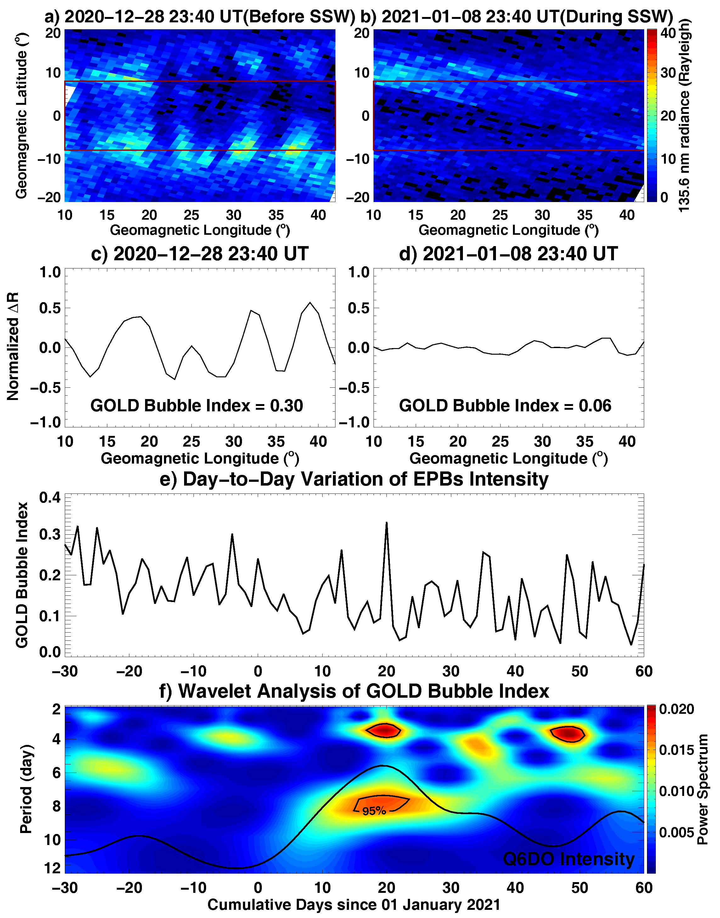
Subsequently, we investigate the day-to-day variability of EPBs observed by the GOLD instrument before and after the beginning of the SSW event. For example, Figure 2a,b shows two GOLD postsunset partial disk images of OI 135.6 nm radiance in geomagnetic coordinates at 23:40 UT on 28 December 2020, a day before the SSW onset, and 8 January 2021, a day during the SSW period. As can be seen, the intensity of EPBs over the American–Atlantic region exhibited a significant difference between these two days: On 28 December 2020, before the onset of the SSW, at least five strong EPBs were noticeable as parallel dark streaks in the equatorial region, elongated in the geomagnetic meridional orientation. However, at the same time on 8 January, after the beginning of the SSW, there were almost no discernible EPBs within the GOLD field of view. To specify the intensity of observed bubbles before and during the SSW for further analysis, Figure 2c,d displays the corresponding longitudinal variation in the normalized differential radiance (ΔR), after removing the latitudinal-integrated reference radiance values within the equatorial rectangle box shown in the top panels. On 28 December (Figure 2c), the curve showed significant fluctuations with five distinct valleys, which effectively delineated the longitudinal variation in EPBs-induced bite-outs in radiance. In contrast, the curve on 8 January (Figure 2d) exhibited very small fluctuations indicating weak/no EPBs. The GOLD Bubble Index is determined as the standard deviation values of the normalized ΔR, which were 0.30 on December 28 and only 0.06 on 8 January, indicating a significant reduction in the intensity of EPBs during the SSW period. For a more detailed mathematical description of the GOLD Bubble Index calculation, readers may refer to [88], which has demonstrated the advantage of this Bubble Index in quantifying the multiday variability of the 2D EPBs’ magnitude in GOLD observations. Given the fact that solar activity was at quite low levels (F10.7 = 84 and 73) and geomagnetic conditions were extremely quiet (Kp ≤ 2) on these two days, external forcing from solar and geomagnetic activities were thus unlikely the causes of such a significant reduction in the intensity of EPBs during the SSW period. Instead, forcing from the lower atmosphere could play an important role.
Moreover, Figure 2e depicts the temporal fluctuation of the GOLD Bubble Index with respect to the cumulative days since 1 January 2021. Following the onset of the SSW, the Bubble Index exhibits a substantial reduction during the period of 5–10 January, significantly lower than that in December 2020. More specifically, the average Bubble Index during the 35 days before the SSW period (i.e., 1 December 2020–4 January 2021) is 0.196, while the average Bubble Index during the 35 days within the SSW period (i.e., 5 January 2021–10 February 2021) is 0.125. This indicates that the intensity of EPBs was notably reduced by approximately 35% during the SSW period. Given that December–January is typically the season with a high occurrence of EPBs over the American–Atlantic sector, it is unlikely that such a significant decrease was solely due to seasonal variations. Moreover, it is known that the occurrence of EPBs can be impacted by solar activity, with a typically higher occurrence rate during solar maximum than during solar minimum [69]. However, solar activity remained at low levels between December 2020 and February 2021, with the average F10.7 index during the pre-SSW and SSW period being 83 and 73 solar flux units, respectively. The significant suppression of observed EPBs is unlikely to be merely caused by small changes in solar flux during this period.
Besides the effects due to seasonal variation and changes in solar flux, such a substantial inhibition of EPBs could be related to the SSW through the following three mechanisms: (1) Suppression of gravity waves seeding. Gravity waves propagating upward could induce wavelike modulations in the electron density and/or polarization electric field at the bottom-side F-region, serving as an important seeding source to initiate the development of EPBs. Several studies have reported that the amplitudes of gravity waves may experience slight enhancements before the reversal of zonal winds at 10 hPa and 60°N but tend to undergo considerable reductions after the onset of SSW, e.g., [103,104,105]. Consequently, the reduction in seeding perturbations caused by gravity waves would effectively suppress the development of EPBs. (2) Changes in the dusk equatorial vertical plasma drifts and in the growth rate of the R-T instability. As previously mentioned in the Introduction, the dusktime equatorial vertical plasma drifts are one of the most critical factors influencing the growth rate of the R-T instability and thus governing the generation of EPBs. Several studies have reported that a phase shift of the migrating semidiurnal tide would cause a reduction in equatorial E × B drifts in the late afternoon during SSW events, e.g., [14,17,79,106], which is considered to be related to the suppression of dusktime PRE. In this study, we further verify this mechanism by examining the variation in equatorial plasma drifts and changes in the growth rate of the R-T instability, as is discussed in the following paragraph. (3) The modification of the flux-tube-integrated conductivity due to variations in meridional neutral winds. It is known that the poleward (equatorward) neutral winds can decrease (increase) the height of the ionospheric layer so as to enhance (reduce) the field-line-integrated Pedersen conductivity, thereby leading to an inhibition (enhancement) of the growth rate of the R-T instability [107]. In particular, Zhang et al. [16] reported poleward disturbances in the field-aligned plasma drift were primarily attributed to the poleward disturbances of meridional winds during the 2021 SSW event. Thus, the poleward neutral wind disturbance tends to reduce the growth rate of the R-T instability, partially contributing to the suppression of EPBs after the onset of SSW.
For an in-depth investigation of the day-to-day variability of EPBs during the SSW period, Figure 2f depicts the wavelet power spectrum of the GOLD Bubble Index with respect to the cumulative days since 1 January 2021. The power spectrum revealed some prominent spectral peaks with a periodicity of 6–8 days and ∼3 days, as circled by the 95% significance lines, as well as some moderate peaks with a quasi-6-day period. Notably, these oscillation components were most noticeable after the onset of SSW from early January through February 2021. In particular, the quasi-6-day spectrum peak observed around 15–20 January corresponds to the period when the zonal winds undergo their most significant reversal at 10 hPa and 60°N, as shown in Figure 1a. Moreover, the black line in Figure 2f represents the temporal variation in the averaged power spectrum with a periodicity of 5.5–8 days (i.e., the Q6DO intensity). As observed, the temporal variation in the Q6DO intensity in EPBs showed a generally consistent trend with that of the Q6DW in the WACCM-X simulation (Figure 1e), both demonstrating a small peak in mid-December and a pronounced enhancement in January with a correlation coefficient of 0.67. This suggests that the amplified planetary wave during this period potentially played a crucial role in modulating the day-to-day variability of EPBs as observed by GOLD.
To explore the potential factors contributing to the significant variability from one day to another day in EPBs during the SSW period, as well as to further validate the connection between planetary waves and ionospheric irregularities, we analyzed the variation in the growth rate of the R-T instability. In order to maximize the utilization of real measurements, we calculated the equatorial localized growth rate of R-T instability at the bottom-side F-region using the equatorial Sao Luis ionosonde measurements on the basis of the following Equation in Sultan [65]:
where is the growth rate of R-T instability; E and B are the magnitude of the zonal electric field, as well as the geomagnetic field, respectively; g represents the gravitational term, and denotes the collision frequency between ion and neutral; is the ionospheric electron density in the F-region; and z is the altitudinal term. It has been demonstrated that this equation is an effective approximation for estimating the localized growth rate of the Rayleigh–Taylor (R-T) instability near the geomagnetic equator, e.g., [63,108,109,110], although its value may be somewhat larger compared with those obtained utilizing flux-tube-integrated values. We note that the term of meridional neutral wind is omitted in the simplified version, partly due to magnetic meridional wind not significantly altering the equatorial conductivity because of the small magnetic inclination angles in that region. The term recombination damping, and other flux-tube-integrated terms, are omitted in this equation due to their either ineffective nature or being less likely to undergo large day-to-day variations [111].
We next employ a similar approach as introduced by [108,109] to calculate the aforementioned parameters by utilizing realistic measurements: the speed factor term (E/B) is substituted with vertical plasma drift data obtained from the Sao Luis digisonde drift mode observations. The inversed vertical gradient scale length of Ne, , is determined based on the Sao Luis digisonde bottom-side electron density profiles. The neutral-ion collision frequency is calculated according to the methodology outlined in Kelley [63] as follows:
where and represent neutral and ion density, respectively, while the variable A is the averaged neutral molecular mass in atomic mass units. These items are computed utilizing the NRLMSISE-00 model [112]. For a more detailed description of this equation, readers could refer to Kelley [63].
Figure 3a,b shows an example of electron density profiles, F2-layer peak height (hmF2), and vertical plasma drift observed by the Sao Luis ionosonde during 4–10 January 2021. Figure 3c illustrates the associated localized growth rate of the R-T instability at the bottom-side F-region that is derived using Sao Luis ionosonde measurements based on Equation (1). The daily peak values of the growth rate were observed after local sunset, attributed to the aforementioned equatorial PRE effect and steep density gradient at the bottom-side F-region in the postsunset hours. Evidently, the postsunset peak values of both the vertical plasma drift and the R-T instability growth rate exhibit a considerable decrease following the onset of the SSW on 5 January. For example, the postsunset peak value of the R-T instability growth rate was about 36 × 10−4/s on 4 January, but largely reduced to around 15–20 × 10−4/s on 7–8 January, and further decreased to 5–10 × 10−4/s on 9–10 January. Such a decreasing trend is consistent with the suppression of EPBs, as shown in Figure 2e. This demonstrates that changes in the amplitudes of PRE during the SSW period play an essential role in modulating the growth rate of the R-T instability, thereby contributing dominantly to the observed inhibition of the intensity of EPBs.
Moreover, Figure 3d,e shows the day-by-day variation in postsunset maximum values of R-T instability growth rate and the corresponding wavelet analysis as a function of the accumulated days since 1 January 2021. As is evident, the wavelet power spectrum exhibits dominant peaks with a periodicity of ∼2–3 days and ∼6 days, particularly noticeable in January through mid-February following the onset of SSW. Additionally, a modest peak with a periodicity of ∼6 days is observed in mid-December. In general, the presence of the Q6DO in the wavelet power spectrum is coincident with the enhancement of Q6DW in the WACCM-X simulation (Figure 1e) and the observed ∼6-day periodicity in the GOLD Bubble Index (Figure 2f); all results exhibit similar predominant spectral peaks in January. This suggests that the amplified Q6DW in the MLT region during the SSW serves as the source of strong ∼6-day oscillations in the R-T instability growth rate and in the day-to-day variation in EPBs. We note that the dominant peak in the GOLD bubble index has a periodicity of 6–8 days, slightly larger than that observed in the R-T instability growth rate. This is because the R-T instability is not equivalent to EPBs, although it is the most pivotal factor determining the development of EPBs. The variability of EPBs is also influenced by potential seeding factors, such as gravity waves and TIDs, as well as forcing from above, such as geomagnetic activities. These factors will further complicate the multiday variability of EPBs, resulting in a slight offset from the dominant 6-day peaks driven by planetary waves.
To further examine the coupling mechanism between the ionosphere and atmosphere, Figure 4 displays the periodogram plot derived from ICON-MIGHTI zonal winds measurements at 100 km altitude from 15 to 30 January 2021. Evident spectrum peaks, especially a quasi-6-day periodicity, could be discerned, suggesting the existence of such periodicity in the ionospheric altitudes, which were coincident with the noticeable Q6DW in the MLT region, as simulated by WACCM-X and consistent with the observed Q6DO signatures in the growth rate of R-T instability and in the intensity of EPBs. These coordinated periodic variations indicate that the observed enhancement of Q6DO in the EPBs during the SSW can be attributed to neutral wind modulations by planetary waves of Q6DW via the ionospheric wind-driven dynamo mechanism.
Figure 5a shows the normalized daily values of the flux-tube-integrated growth rate of R-T instability and the PRE averaged between 20–120°W longitudes, derived from the WACCM-X simulations (LA only). Figure 5b depicts the cross-correlation analysis of the PRE and R-T instability. As observed, the two parameters exhibit significant common powers manifested as encircled spectral peaks in mid-December 2020 and January 2021, generally coinciding with that of the enhanced Q6DW in the MLT region shown in Figure 1e, although the connection appears to be nonlinear. The arrows within the common power region mainly point to the right, indicating an in-phase variation between PRE and R-T instability, as expected. The spectral peak region in January exhibits a dominant periodicity of 5–7 days, consistent with that of the ICON wind measurements as shown in Figure 4 and the localized R-T instability growth rate, as shown in Figure 3e. Pedatella et al. [86] has shown that the amplitude of semidiurnal migrating tides exhibits a distinct spectral peak, with a periodicity of approximately 6 days after the onset of the SSW, consistent with the timing of enhanced Q6DW in the MLT region. Therefore, we deduce that the Q6DW in the MLT region acted to induce periodic oscillations in the zonal winds through interaction with semidiurnal migrating tides, which subsequently modulated the strength of PRE via the E-region wind-driven dynamo at a similar periodicity, leading to the observed Q6DO in the growth rate of the R-T instability and ultimately modulating the intensity of EPBs.
4. Conclusions
This study uses multi-instrument observations and the WACCM-X simulation to investigate the day-to-day variability of EPBs and their relationship to atmospheric planetary waves during the 2021 SSW event. The main findings are as follows:
- We found that the intensity of EPBs was notably reduced by 35% during the SSW period compared with the non-SSW period. Such a significant inhibition of EPBs during the SSW period could be collectively attributed to the suppression of gravity waves seeding, changes in the dusk equatorial vertical plasma drifts and in the growth rate of the R-T instability, and the modification of Pedersen conductivity due to the variations in neutral winds. In addition to SSW, there could also be some effects due to seasonal variations and changes in solar flux.
- We found that significant Q6DO signatures were observed in both the intensity of EPBs and the associated growth rate of R-T instability during the SSW, which were coincident with the amplification of the Q6DW in the WACCM-X simulation and noticeable ∼6-day periodicity in ICON-MIGHTI zonal winds. These results demonstrate that certain planetary waves like the Q6DW can play a crucial role in controlling the day-to-day variability of EPBs, especially during the SSW event. This influence is exerted through the modulation of zonal winds and the ionospheric E-region dynamo via the interaction between planetary waves and tides, which led to periodic oscillations in the PRE strength and the growth rate of the R-T instability, ultimately resulting in the Q6DO in the intensity of EPBs. These findings provide new insights into the day-to-day variability of ionospheric irregularities and their potential correlation with atmospheric planetary waves.
Author Contributions
Conceptualization, E.A. and N.M.P.; methodology, E.A. and N.M.P.; software, N.M.P.; validation, E.A., N.M.P. and G.L.; formal analysis, E.A. and N.M.P.; investigation, E.A. and N.M.P.; resources, N.M.P.; writing—original draft preparation, E.A.; writing—review and editing, N.M.P. and G.L.; visualization, E.A.; supervision, N.M.P.; project administration, E.A.; funding acquisition, E.A. and N.M.P. All authors have read and agreed to the published version of the manuscript.
Funding
This work is supported by NSF awards AGS-1952737, AGS-2033787, PHY-2028125, and NSFC41974184, NASA support 80NSSC22K0171, 80NSSC21K1310, 80GSFC22CA011, NNH220B82A, and NNH17ZDA001N07.
Data Availability Statement
GOLD data can be accessed at (https://gold.cs.ucf.edu/data/search/ (accessed on 1 January 2024)). The ionosonde data are provided by the University of Massachusetts Lowell DIDB database of Global Ionospheric Radio Observatory (https://giro.uml.edu/didbase/scaled.php (accessed on 1 January 2024)). The NCEP stratosphere reanalysis data can be accessed at NASA Atmospheric Chemistry and Dynamics Laboratory (https://acd-ext.gsfc.nasa.gov/Data_services/met/ann_data.html (accessed on 1 January 2024)).
Acknowledgments
WACCM-X is part of the Community Earth System Model (CESM) and the source code is available at (http://www.cesm.ucar.edu (accessed on 1 January 2024)).
Conflicts of Interest
The authors declare no conflicts of interest.
References
- Forbes, J.M.; Palo, S.E.; Zhang, X. Variability of the ionosphere. J. Atmos. Sol. Terr. Phys. 2000, 62, 685–693. [Google Scholar] [CrossRef]
- Liu, H.L. Variability and predictability of the space environment as related to lower atmosphere forcing. Space Weather 2016, 14, 634–658. [Google Scholar] [CrossRef]
- Matsuno, T. A Dynamical Model of the Stratospheric Sudden Warming. J. Atmos. Sci. 1971, 28, 1479–1494. [Google Scholar] [CrossRef]
- Baldwin, M.P.; Ayarzagüena, B.; Birner, T.; Butchart, N.; Butler, A.H.; Charlton-Perez, A.J.; Domeisen, D.I.V.; Garfinkel, C.I.; Garny, H.; Gerber, E.P.; et al. Sudden Stratospheric Warmings. Rev. Geophys. 2021, 59, e2020RG000708. [Google Scholar] [CrossRef]
- Goncharenko, L.P.; Harvey, V.L.; Liu, H.; Pedatella, N.M. Sudden Stratospheric Warming Impacts on the Ionosphere-Thermosphere System: A Review of Recent Progress. In Proceedings of the Ionosphere Dynamics and Applications; Huang, C., Lu, G., Eds.; AGU Publications: Washington, DC, USA, 2021; Volume 3, p. 369. [Google Scholar] [CrossRef]
- Pedatella, N.M.; Chau, J.; Schmidt, H.; Goncharenko, L.; Stolle, C.; Hocke, K.; Harvey, V.; Funke, B.; Siddiqui, T. How sudden stratospheric warming affects the whole atmosphere. EOS 2018, 99, 35–38. [Google Scholar] [CrossRef]
- Forbes, J.M.; Zhang, X. Lunar tide amplification during the January 2009 stratosphere warming event: Observations and theory. J. Geophys. Res. Space Phys. 2012, 117, A12312. [Google Scholar] [CrossRef]
- Zhang, X.; Forbes, J.M. Lunar tide in the thermosphere and weakening of the northern polar vortex. Geophys. Res. Lett. 2014, 41, 8201–8207. [Google Scholar] [CrossRef]
- Chau, J.L.; Goncharenko, L.P.; Fejer, B.G.; Liu, H.L. Equatorial and Low Latitude Ionospheric Effects During Sudden Stratospheric Warming Events. Ionospheric Effects During SSW Events. Space Sci. Rev. 2012, 168, 385–417. [Google Scholar] [CrossRef]
- Chau, J.L.; Fejer, B.G.; Goncharenko, L.P. Quiet variability of equatorial E × B drifts during a sudden stratospheric warming event. Geophys. Res. Lett. 2009, 36, L05101. [Google Scholar] [CrossRef]
- Fang, T.W.; Fuller-Rowell, T.; Wang, H.; Akmaev, R.; Wu, F. Ionospheric response to sudden stratospheric warming events at low and high solar activity. J. Geophys. Res. Space Phys. 2014, 119, 7858–7869. [Google Scholar] [CrossRef]
- Fejer, B.G.; Tracy, B.D.; Olson, M.E.; Chau, J.L. Enhanced lunar semidiurnal equatorial vertical plasma drifts during sudden stratospheric warmings. Geophys. Res. Lett. 2011, 38, L21104. [Google Scholar] [CrossRef]
- Goncharenko, L.P.; Chau, J.L.; Liu, H.L.; Coster, A.J. Unexpected connections between the stratosphere and ionosphere. Geophys. Res. Lett. 2010, 37, L10101. [Google Scholar] [CrossRef]
- Maute, A.; Hagan, M.E.; Richmond, A.D.; Roble, R.G. TIME-GCM study of the ionospheric equatorial vertical drift changes during the 2006 stratospheric sudden warming. J. Geophys. Res. Space Phys. 2014, 119, 1287–1305. [Google Scholar] [CrossRef]
- Maute, A.; Fejer, B.G.; Forbes, J.M.; Zhang, X.; Yudin, V. Equatorial vertical drift modulation by the lunar and solar semidiurnal tides during the 2013 sudden stratospheric warming. J. Geophys. Res. Space Phys. 2016, 121, 1658–1668. [Google Scholar] [CrossRef]
- Zhang, R.; Liu, L.; Ma, H.; Chen, Y.; Le, H. ICON Observations of Equatorial Ionospheric Vertical ExB and Field-Aligned Plasma Drifts During the 2020-2021 SSW. Geophys. Res. Lett. 2022, 49, e99238. [Google Scholar] [CrossRef]
- Fejer, B.G.; Olson, M.E.; Chau, J.L.; Stolle, C.; Lühr, H.; Goncharenko, L.P.; Yumoto, K.; Nagatsuma, T. Lunar-dependent equatorial ionospheric electrodynamic effects during sudden stratospheric warmings. J. Geophys. Res. Space Phys. 2010, 115, A00G03. [Google Scholar] [CrossRef]
- Park, J.; Lühr, H.; Kunze, M.; Fejer, B.G.; Min, K.W. Effect of sudden stratospheric warming on lunar tidal modulation of the equatorial electrojet. J. Geophys. Res. Space Phys. 2012, 117, A03306. [Google Scholar] [CrossRef]
- Patra, A.K.; Pavan Chaitanya, P.; Sripathi, S.; Alex, S. Ionospheric variability over Indian low latitude linked with the 2009 sudden stratospheric warming. J. Geophys. Res. Space Phys. 2014, 119, 4044–4061. [Google Scholar] [CrossRef]
- Siddiqui, T.A.; Maute, A.; Pedatella, N.; Yamazaki, Y.; Lühr, H.; Stolle, C. On the variability of the semidiurnal solar and lunar tides of the equatorial electrojet during sudden stratospheric warmings. Ann. Geophys. 2018, 36, 1545–1562. [Google Scholar] [CrossRef]
- Yamazaki, Y.; Yumoto, K.; McNamara, D.; Hirooka, T.; Uozumi, T.; Kitamura, K.; Abe, S.; Ikeda, A. Ionospheric current system during sudden stratospheric warming events. J. Geophys. Res. Space Phys. 2012, 117, A03334. [Google Scholar] [CrossRef]
- Fagundes, P.R.; Goncharenko, L.P.; Abreu, A.J.; Venkatesh, K.; Pezzopane, M.; Jesus, R.; Gende, M.; Coster, A.J.; Pillat, V.G. Ionospheric response to the 2009 sudden stratospheric warming over the equatorial, low, and middle latitudes in the South American sector. J. Geophys. Res. Space Phys. 2015, 120, 7889–7902. [Google Scholar] [CrossRef]
- Jin, H.; Miyoshi, Y.; Pancheva, D.; Mukhtarov, P.; Fujiwara, H.; Shinagawa, H. Response of migrating tides to the stratospheric sudden warming in 2009 and their effects on the ionosphere studied by a whole atmosphere-ionosphere model GAIA with COSMIC and TIMED/SABER observations. J. Geophys. Res. Space Phys. 2012, 117, A10323. [Google Scholar] [CrossRef]
- Lin, C.H.; Lin, J.T.; Chang, L.C.; Liu, J.Y.; Chen, C.H.; Chen, W.H.; Huang, H.H.; Liu, C.H. Observations of global ionospheric responses to the 2009 stratospheric sudden warming event by FORMOSAT-3/COSMIC. J. Geophys. Res. Space Phys. 2012, 117, A06323. [Google Scholar] [CrossRef]
- Liu, H.; Yamamoto, M.; Tulasi Ram, S.; Tsugawa, T.; Otsuka, Y.; Stolle, C.; Doornbos, E.; Yumoto, K.; Nagatsuma, T. Equatorial electrodynamics and neutral background in the Asian sector during the 2009 stratospheric sudden warming. J. Geophys. Res. Space Phys. 2011, 116, A08308. [Google Scholar] [CrossRef]
- Oberheide, J. Day-to-Day Variability of the Semidiurnal Tide in the F-Region Ionosphere During the January 2021 SSW From COSMIC-2 and ICON. Geophys. Res. Lett. 2022, 49, e00369. [Google Scholar] [CrossRef]
- Pancheva, D.; Mukhtarov, P. Stratospheric warmings: The atmosphere-ionosphere coupling paradigm. J. Atmos.-Sol.-Terr. Phys. 2011, 73, 1697–1702. [Google Scholar] [CrossRef]
- Pedatella, N.M.; Forbes, J.M. Evidence for stratosphere sudden warming-ionosphere coupling due to vertically propagating tides. Geophys. Res. Lett. 2010, 37, L11104. [Google Scholar] [CrossRef]
- Gan, Q.; Eastes, R.W.; Burns, A.G.; Wang, W.; Qian, L.; Solomon, S.C.; Codrescu, M.V.; McClintock, W.E. New Observations of Large-Scale Waves Coupling With the Ionosphere Made by the GOLD Mission: Quasi-16-Day Wave Signatures in the F-Region OI 135.6-nm Nightglow During Sudden Stratospheric Warmings. J. Geophys. Res. Space Phys. 2020, 125, e27880. [Google Scholar] [CrossRef]
- Gu, S.Y.; Li, T.; Dou, X.; Wu, Q.; Mlynczak, M.G.; Russell, J.M. Observations of Quasi-Two-Day wave by TIMED/SABER and TIMED/TIDI. J. Geophys. Res. Atmos. 2013, 118, 1624–1639. [Google Scholar] [CrossRef]
- Liu, G.; England, S.L.; Janches, D. Quasi Two-, Three-, and Six-Day Planetary-Scale Wave Oscillations in the Upper Atmosphere Observed by TIMED/SABER Over 17 Years During 2002-2018. J. Geophys. Res. Space Phys. 2019, 124, 9462–9474. [Google Scholar] [CrossRef]
- Mo, X.; Zhang, D. Quasi-10 d wave modulation of an equatorial ionization anomaly during the Southern Hemisphere stratospheric warming of 2002. Ann. Geophys. 2020, 38, 9–16. [Google Scholar] [CrossRef]
- Vineeth, C.; Pant, T.K.; Sridharan, R. Equatorial counter electrojets and polar stratospheric sudden warmings—A classical example of high latitude-low latitude coupling? Ann. Geophys. 2009, 27, 3147–3153. [Google Scholar] [CrossRef]
- Yamazaki, Y.; Matthias, V.; Miyoshi, Y.; Stolle, C.; Siddiqui, T.; Kervalishvili, G.; Laštovička, J.; Kozubek, M.; Ward, W.; Themens, D.R.; et al. September 2019 Antarctic Sudden Stratospheric Warming: Quasi-6-Day Wave Burst and Ionospheric Effects. Geophys. Res. Lett. 2020, 47, e86577. [Google Scholar] [CrossRef]
- Yue, J.; Wang, W.; Ruan, H.; Chang, L.C.; Lei, J. Impact of the interaction between the quasi-2 day wave and tides on the ionosphere and thermosphere. J. Geophys. Res. Space Phys. 2016, 121, 3555–3563. [Google Scholar] [CrossRef]
- Forbes, J.M.; Maute, A.; Zhang, X.; Hagan, M.E. Oscillation of the Ionosphere at Planetary-Wave Periods. J. Geophys. Res. Space Phys. 2018, 123, 7634–7649. [Google Scholar] [CrossRef]
- Laštovička, J. Forcing of the ionosphere by waves from below. J. Atmos.-Sol.-Terr. Phys. 2006, 68, 479–497. [Google Scholar] [CrossRef]
- Pancheva, D.; Merzlyakov, E.; Mitchell, N.J.; Portnyagin, Y.; Manson, A.H.; Jacobi, C.; Meek, C.E.; Luo, Y.; Clark, R.R.; Hocking, W.K.; et al. Global-scale tidal variability during the PSMOS campaign of June–August 1999: Interaction with planetary waves. J. Atmos.-Sol.-Terr. Phys. 2002, 64, 1865–1896. [Google Scholar] [CrossRef]
- Lieberman, R.S.; Riggin, D.M.; Franke, S.J.; Manson, A.H.; Meek, C.; Nakamura, T.; Tsuda, T.; Vincent, R.A.; Reid, I. The 6.5-day wave in the mesosphere and lower thermosphere: Evidence for baroclinic/barotropic instability. J. Geophys. Res. Atmos. 2003, 108, 4640. [Google Scholar] [CrossRef]
- Liu, H.L.; Talaat, E.R.; Roble, R.G.; Lieberman, R.S.; Riggin, D.M.; Yee, J.H. The 6.5-day wave and its seasonal variability in the middle and upper atmosphere. J. Geophys. Res. Atmos. 2004, 109, D21112. [Google Scholar] [CrossRef]
- Talaat, E.R.; Yee, J.H.; Zhu, X. The 6.5-day wave in the tropical stratosphere and mesosphere. J. Geophys. Res. Atmos. 2002, 107, 4133. [Google Scholar] [CrossRef]
- Wu, D.L.; Hays, P.B.; Skinner, W.R. Observations of the 5-day wave in the mesosphere and lower thermosphere. Geophys. Res. Lett. 1994, 21, 2733–2736. [Google Scholar] [CrossRef]
- Gan, Q.; Oberheide, J.; Pedatella, N.M. Sources, Sinks, and Propagation Characteristics of the Quasi 6-Day Wave and Its Impact on the Residual Mean Circulation. J. Geophys. Res. Atmos. 2018, 123, 9152–9170. [Google Scholar] [CrossRef]
- Gu, S.Y.; Ruan, H.; Yang, C.Y.; Gan, Q.; Dou, X.; Wang, N. The Morphology of the 6-Day Wave in Both the Neutral Atmosphere and F Region Ionosphere Under Solar Minimum Conditions. J. Geophys. Res. Space Phys. 2018, 123, 4232–4240. [Google Scholar] [CrossRef]
- Lin, J.T.; Lin, C.H.; Rajesh, P.K.; Yue, J.; Lin, C.Y.; Matsuo, T. Local-Time and Vertical Characteristics of Quasi-6-Day Oscillation in the Ionosphere During the 2019 Antarctic Sudden Stratospheric Warming. Geophys. Res. Lett. 2020, 47, e90345. [Google Scholar] [CrossRef]
- Qin, Y.; Gu, S.Y.; Dou, X.; Gong, Y.; Chen, G.; Zhang, S.; Wu, Q. Climatology of the Quasi-6-Day Wave in the Mesopause Region and Its Modulations on Total Electron Content During 2003-2017. J. Geophys. Res. Space Phys. 2019, 124, 573–583. [Google Scholar] [CrossRef]
- Yamazaki, Y. Quasi-6-Day Wave Effects on the Equatorial Ionization Anomaly Over a Solar Cycle. J. Geophys. Res. Space Phys. 2018, 123, 9881–9892. [Google Scholar] [CrossRef]
- Chang, L.C.; Yue, J.; Wang, W.; Wu, Q.; Meier, R.R. Quasi two day wave-related variability in the background dynamics and composition of the mesosphere/thermosphere and the ionosphere. J. Geophys. Res. Space Phys. 2014, 119, 4786–4804. [Google Scholar] [CrossRef] [PubMed]
- Kil, H. The Morphology of Equatorial Plasma Bubbles—A review. J. Astron. Space Sci. 2015, 32, 13–19. [Google Scholar] [CrossRef]
- Woodman, R.F.; La Hoz, C. Radar observations of F region equatorial irregularities. J. Geophys. Res. 1976, 81, 5447–5466. [Google Scholar] [CrossRef]
- Hysell, D.L. An overview and synthesis of plasma irregularities in equatorial spread/F. J. Atmos. Sol. Terr. Phys. 2000, 62, 1037–1056. [Google Scholar] [CrossRef]
- Aa, E.; Huang, W.; Liu, S.; Ridley, A.; Zou, S.; Shi, L.; Chen, Y.; Shen, H.; Yuan, T.; Li, J.; et al. Midlatitude Plasma Bubbles Over China and Adjacent Areas During a Magnetic Storm on 8 September 2017. Space Weather 2018, 16, 321–331. [Google Scholar] [CrossRef]
- Aa, E.; Zou, S.; Ridley, A.; Zhang, S.; Coster, A.J.; Erickson, P.J.; Liu, S.; Ren, J. Merging of Storm Time Midlatitude Traveling Ionospheric Disturbances and Equatorial Plasma Bubbles. Space Weather 2019, 17, 285–298. [Google Scholar] [CrossRef]
- Abdu, M.A.; Batista, P.P.; Batista, I.S.; Brum, C.G.M.; Carrasco, A.J.; Reinisch, B.W. Planetary wave oscillations in mesospheric winds, equatorial evening prereversal electric field and spread F. Geophys. Res. Lett. 2006, 33, L07107. [Google Scholar] [CrossRef]
- Huang, C.S.; Hairston, M.R. The postsunset vertical plasma drift and its effects on the generation of equatorial plasma bubbles observed by the C/NOFS satellite. J. Geophys. Res. Space Phys. 2015, 120, 2263–2275. [Google Scholar] [CrossRef]
- Huba, J.D.; Joyce, G. Global modeling of equatorial plasma bubbles. Geophys. Res. Lett. 2010, 37, L17104. [Google Scholar] [CrossRef]
- Karan, D.K.; Eastes, R.W.; Daniell, R.E.; Martinis, C.R.; McClintock, W.E. GOLD Mission’s Observation About the Geomagnetic Storm Effects on the Nighttime Equatorial Ionization Anomaly (EIA) and Equatorial Plasma Bubbles (EPB) During a Solar Minimum Equinox. Space Weather 2023, 21, e2022SW003321. [Google Scholar] [CrossRef]
- Klenzing, J.; Halford, A.J.; Liu, G.; Smith, J.M.; Zhang, Y.; Zawdie, K.; Maruyama, N.; Pfaff, R.; Bishop, R.L. A system science perspective of the drivers of equatorial plasma bubbles. Front. Astron. Space Sci. 2023, 9, 420. [Google Scholar] [CrossRef]
- Li, G.; Ning, B.; Liu, L.; Wan, W.; Liu, J.Y. Effect of magnetic activity on plasma bubbles over equatorial and low-latitude regions in East Asia. Ann. Geophys. 2009, 27, 303–312. [Google Scholar] [CrossRef]
- Makela, J.J.; Vadas, S.L.; Muryanto, R.; Duly, T.; Crowley, G. Periodic spacing between consecutive equatorial plasma bubbles. Geophys. Res. Lett. 2010, 37, L14103. [Google Scholar] [CrossRef]
- Otsuka, Y.; Shiokawa, K.; Ogawa, T.; Wilkinson, P. Geomagnetic conjugate observations of equatorial airglow depletions. Geophys. Res. Lett. 2002, 29, 1753. [Google Scholar] [CrossRef]
- Yokoyama, T.; Shinagawa, H.; Jin, H. Nonlinear growth, bifurcation, and pinching of equatorial plasma bubble simulated by three-dimensional high-resolution bubble model. J. Geophys. Res. Space Phys. 2014, 119, 10474–10482. [Google Scholar] [CrossRef]
- Kelley, M.C. Equatorial Plasma Instabilities. In The Earth’s Ionosphere: Plasma Physics and Electrodynamics; Kelley, M.C., Ed.; Academic Press: Cambridge, MA, USA, 1989; pp. 113–185. [Google Scholar] [CrossRef]
- Ott, E. Theory of Rayleigh-Taylor bubbles in the equatorial ionosphere. J. Geophys. Res. 1978, 83, 2066–2070. [Google Scholar] [CrossRef]
- Sultan, P.J. Linear theory and modeling of the Rayleigh-Taylor instability leading to the occurrence of equatorial spread F. J. Geophys. Res. 1996, 101, 26875–26892. [Google Scholar] [CrossRef]
- Abadi, P.; Otsuka, Y.; Tsugawa, T. Effects of pre-reversal enhancement of E × B drift on the latitudinal extension of plasma bubble in Southeast Asia. Earth Planets Space 2015, 67, 74. [Google Scholar] [CrossRef]
- Fejer, B.G.; Scherliess, L.; de Paula, E.R. Effects of the vertical plasma drift velocity on the generation and evolution of equatorial spread F. J. Geophys. Res. 1999, 104, 19859–19870. [Google Scholar] [CrossRef]
- Huang, C.S. Effects of the postsunset vertical plasma drift on the generation of equatorial spread F. Prog. Earth Planet. Sci. 2018, 5, 3. [Google Scholar] [CrossRef]
- Aa, E.; Zou, S.; Liu, S. Statistical Analysis of Equatorial Plasma Irregularities Retrieved From Swarm 2013-2019 Observations. J. Geophys. Res. Space Phys. 2020, 125, e27022. [Google Scholar] [CrossRef]
- Burke, W.J.; Gentile, L.C.; Huang, C.Y.; Valladares, C.E.; Su, S.Y. Longitudinal variability of equatorial plasma bubbles observed by DMSP and ROCSAT-1. J. Geophys. Res. Space Phys. 2004, 109, A12301. [Google Scholar] [CrossRef]
- Gentile, L.C.; Burke, W.J.; Rich, F.J. A global climatology for equatorial plasma bubbles in the topside ionosphere. Ann. Geophys. 2006, 24, 163–172. [Google Scholar] [CrossRef]
- Smith, J.; Heelis, R.A. Equatorial plasma bubbles: Variations of occurrence and spatial scale in local time, longitude, season, and solar activity. J. Geophys. Res. Space Phys. 2017, 122, 5743–5755. [Google Scholar] [CrossRef]
- Su, S.Y.; Chao, C.K.; Liu, C.H. On monthly/seasonal/longitudinal variations of equatorial irregularity occurrences and their relationship with the postsunset vertical drift velocities. J. Geophys. Res. Space Phys. 2008, 113, A05307. [Google Scholar] [CrossRef]
- Wan, X.; Xiong, C.; Rodriguez-Zuluaga, J.; Kervalishvili, G.N.; Stolle, C.; Wang, H. Climatology of the Occurrence Rate and Amplitudes of Local Time Distinguished Equatorial Plasma Depletions Observed by Swarm Satellite. J. Geophys. Res. Space Phys. 2018, 123, 3014–3026. [Google Scholar] [CrossRef]
- Abdu, M.A. Day-to-day and short-term variabilities in the equatorial plasma bubble/spread F irregularity seeding and development. Prog. Earth Planet. Sci. 2019, 6, 11. [Google Scholar] [CrossRef]
- Retterer, J.M.; Roddy, P. Faith in a seed: On the origins of equatorial plasma bubbles. Ann. Geophys. 2014, 32, 485–498. [Google Scholar] [CrossRef]
- Tsunoda, R.T. On the enigma of day-to-day variability in equatorial spread F. Geophys. Res. Lett. 2005, 32, L08103. [Google Scholar] [CrossRef]
- Tsunoda, R.T. Day-to-day variability in equatorial spread F: Is there some physics missing? Geophys. Res. Lett. 2006, 33, L16106. [Google Scholar] [CrossRef]
- de Paula, E.R.; Jonah, O.F.; Moraes, A.O.; Kherani, E.A.; Fejer, B.G.; Abdu, M.A.; Muella, M.T.A.H.; Batista, I.S.; Dutra, S.L.G.; Paes, R.R. Low-latitude scintillation weakening during sudden stratospheric warming events. J. Geophys. Res. Space Phys. 2015, 120, 2212–2221. [Google Scholar] [CrossRef]
- Yu, T.; Ye, H.; Liu, H.; Xia, C.; Zuo, X.; Yan, X.; Yang, N.; Sun, Y.; Zhao, B. Ionospheric F Layer Scintillation Weakening as Observed by COSMIC/FORMOSAT-3 During the Major Sudden Stratospheric Warming in January 2013. J. Geophys. Res. Space Phys. 2020, 125, e27721. [Google Scholar] [CrossRef]
- Ye, H.; Xue, X.; Yu, T.; Sun, Y.Y.; Yi, W.; Long, C.; Zhang, W.; Dou, X. Ionospheric F-Layer Scintillation Variabilities Over the American Sector During Sudden Stratospheric Warming Events. Space Weather 2021, 19, e2020SW002703. [Google Scholar] [CrossRef]
- Jose, L.; Vineeth, C.; Pant, T.K. Impact of Stratospheric Sudden Warming on the Occurrence of the Equatorial Spread-F. J. Geophys. Res. Space Phys. 2017, 122, 12544–12555. [Google Scholar] [CrossRef]
- Abdu, M.A.; Brum, C.G.; Batista, P.P.; Gurubaran, S.; Pancheva, D.; Bageston, J.V.; Batista, I.S.; Takahashi, H. Fast and ultrafast Kelvin wave modulations of the equatorial evening F region vertical drift and spread F development. Earth Planets Space 2015, 67, 1. [Google Scholar] [CrossRef]
- Ghosh, P.; Otsuka, Y.; Mani, S.; Shinagawa, H. Day-to-day variation of pre-reversal enhancement in the equatorial ionosphere based on GAIA model simulations. Earth Planets Space 2020, 72, 93. [Google Scholar] [CrossRef]
- Liu, H.L. Day-to-Day Variability of Prereversal Enhancement in the Vertical Ion Drift in Response to Large-Scale Forcing From the Lower Atmosphere. Space Weather 2020, 18, e02334. [Google Scholar] [CrossRef]
- Pedatella, N.M.; Aa, E.; Maute, A. Quasi 6-Day Planetary Wave Oscillations in Equatorial Plasma Irregularities. J. Geophys. Res. Space Phys. 2024, 129, e2023JA032312. [Google Scholar] [CrossRef]
- Yamazaki, Y.; Diéval, C. Modeling of Planetary Wave Influences on the Pre reversal Enhancement of the Equatorial F Region Vertical Plasma Drift. Space Weather 2021, 19, e02685. [Google Scholar] [CrossRef]
- Aa, E.; Zhang, S.R.; Liu, G.; Eastes, R.W.; Wang, W.; Karan, D.K.; Qian, L.; Coster, A.J.; Erickson, P.J.; Derghazarian, S. Statistical Analysis of Equatorial Plasma Bubbles Climatology and Multi-Day Periodicity Using GOLD Observations. Geophys. Res. Lett. 2023, 50, e2023GL103510. [Google Scholar] [CrossRef]
- Eastes, R.W.; McClintock, W.E.; Burns, A.G.; Anderson, D.N.; Andersson, L.; Codrescu, M.; Correira, J.T.; Daniell, R.E.; England, S.L.; Evans, J.S.; et al. The Global-Scale Observations of the Limb and Disk (GOLD) Mission. Space Sci. Rev. 2017, 212, 383–408. [Google Scholar] [CrossRef]
- Eastes, R.W.; Solomon, S.C.; Daniell, R.E.; Anderson, D.N.; Burns, A.G.; England, S.L.; Martinis, C.R.; McClintock, W.E. Global-Scale Observations of the Equatorial Ionization Anomaly. Geophys. Res. Lett. 2019, 46, 9318–9326. [Google Scholar] [CrossRef]
- Aa, E.; Zou, S.; Eastes, R.; Karan, D.K.; Zhang, S.R.; Erickson, P.J.; Coster, A.J. Coordinated Ground-Based and Space-Based Observations of Equatorial Plasma Bubbles. J. Geophys. Res. Space Phys. 2020, 125, e27569. [Google Scholar] [CrossRef]
- Aa, E.; Zhang, S.R.; Erickson, P.J.; Wang, W.; Qian, L.; Cai, X.; Coster, A.J.; Goncharenko, L.P. Significant Mid- and Low-Latitude Ionospheric Disturbances Characterized by Dynamic EIA, EPBs, and SED Variations During the 13–14 March 2022 Geomagnetic Storm. J. Geophys. Res. Space Phys. 2023, 128, e2023JA031375. [Google Scholar] [CrossRef]
- Eastes, R.W.; McClintock, W.E.; Burns, A.G.; Anderson, D.N.; Andersson, L.; Aryal, S.; Budzien, S.A.; Cai, X.; Codrescu, M.V.; Correira, J.T.; et al. Initial Observations by the GOLD Mission. J. Geophys. Res. Space Phys. 2020, 125, e27823. [Google Scholar] [CrossRef]
- Martinis, C.; Daniell, R.; Eastes, R.; Norrell, J.; Smith, J.; Klenzing, J.; Solomon, S.; Burns, A. Longitudinal Variation of Postsunset Plasma Depletions From the Global Scale Observations of the Limb and Disk (GOLD) Mission. J. Geophys. Res. Space Phys. 2021, 126, e28510. [Google Scholar] [CrossRef]
- Immel, T.J.; England, S.L.; Mende, S.B.; Heelis, R.A.; Englert, C.R.; Edelstein, J.; Frey, H.U.; Korpela, E.J.; Taylor, E.R.; Craig, W.W.; et al. The Ionospheric Connection Explorer Mission: Mission Goals and Design. Space Sci. Rev. 2018, 214, 13. [Google Scholar] [CrossRef] [PubMed]
- Harding, B.J.; Makela, J.J.; Englert, C.R.; Marr, K.D.; Harlander, J.M.; England, S.L.; Immel, T.J. The MIGHTI Wind Retrieval Algorithm: Description and Verification. Space Sci. Rev. 2017, 212, 585–600. [Google Scholar] [CrossRef] [PubMed]
- Liu, G.; England, S.L.; Lin, C.S.; Pedatella, N.M.; Klenzing, J.H.; Englert, C.R.; Harding, B.J.; Immel, T.J.; Rowland, D.E. Evaluation of Atmospheric 3-Day Waves as a Source of Day-to-Day Variation of the Ionospheric Longitudinal Structure. Geophys. Res. Lett. 2021, 48, e94877. [Google Scholar] [CrossRef]
- Liu, H.L.; Bardeen, C.G.; Foster, B.T.; Lauritzen, P.; Liu, J.; Lu, G.; Marsh, D.R.; Maute, A.; McInerney, J.M.; Pedatella, N.M.; et al. Development and Validation of the Whole Atmosphere Community Climate Model with Thermosphere and Ionosphere Extension (WACCM-X 2.0). J. Adv. Model. Earth Syst. 2018, 10, 381–402. [Google Scholar] [CrossRef]
- Pedatella, N.M. Ionospheric Variability during the 2020-2021 SSW: COSMIC-2 Observations and WACCM-X Simulations. Atmosphere 2022, 13, 368. [Google Scholar] [CrossRef]
- Gelaro, R.; McCarty, W.; Suárez, M.J.; Todling, R.; Molod, A.; Takacs, L.; Randles, C.A.; Darmenov, A.; Bosilovich, M.G.; Reichle, R.; et al. The Modern-Era Retrospective Analysis for Research and Applications, Version 2 (MERRA-2). J. Clim. 2017, 30, 5419–5454. [Google Scholar] [CrossRef] [PubMed]
- Heelis, R.A.; Lowell, J.K.; Spiro, R.W. A model of the high-latitude ionospheric convection pattern. J. Geophys. Res. 1982, 87, 6339–6345. [Google Scholar] [CrossRef]
- Liu, J.; Zhang, D.; Sun, S.; Hao, Y.; Xiao, Z. Ionospheric Semidiurnal Lunitidal Perturbations During the 2021 Sudden Stratospheric Warming Event: Latitudinal and Inter-Hemispheric Variations in the American, Asian-Australian, and African-European Sectors. J. Geophys. Res. Space Phys. 2022, 127, e2022JA030313. [Google Scholar] [CrossRef]
- Nayak, C.; Yiǧit, E. Variation of Small-Scale Gravity Wave Activity in the Ionosphere During the Major Sudden Stratospheric Warming Event of 2009. J. Geophys. Res. Space Phys. 2019, 124, 470–488. [Google Scholar] [CrossRef]
- Thurairajah, B.; Bailey, S.M.; Cullens, C.Y.; Hervig, M.E.; Russell, J.M. Gravity wave activity during recent stratospheric sudden warming events from SOFIE temperature measurements. J. Geophys. Res. Atmos. 2014, 119, 8091–8103. [Google Scholar] [CrossRef]
- Yamashita, C.; Liu, H.L.; Chu, X. Gravity wave variations during the 2009 stratospheric sudden warming as revealed by ECMWF-T799 and observations. Geophys. Res. Lett. 2010, 37, L22806. [Google Scholar] [CrossRef]
- Pedatella, N.M.; Liu, H.L. The influence of atmospheric tide and planetary wave variability during sudden stratosphere warmings on the low latitude ionosphere. J. Geophys. Res. Space Phys. 2013, 118, 5333–5347. [Google Scholar] [CrossRef]
- Maruyama, T. A diagnostic model for equatorial spread F. 1. Model description and application to electric field and neutral wind effects. J. Geophys. Res. 1988, 93, 14611–14622. [Google Scholar] [CrossRef]
- Aa, E.; Zhang, S.R.; Coster, A.J.; Erickson, P.J.; Rideout, W. Multi-instrumental analysis of the day-to-day variability of equatorial plasma bubbles. Front. Astron. Space Sci. 2023, 10, 1167245. [Google Scholar] [CrossRef]
- Das, S.K.; Patra, A.K.; Niranjan, K. On the Assessment of Day To Day Occurrence of Equatorial Plasma Bubble. J. Geophys. Res. Space Phys. 2021, 126, e29129. [Google Scholar] [CrossRef]
- Otsuka, Y. Review of the generation mechanisms of post-midnight irregularities in the equatorial and low-latitude ionosphere. Prog. Earth Planet. Sci. 2018, 5, 57. [Google Scholar] [CrossRef]
- Huba, J.D.; Bernhardt, P.A.; Ossakow, S.L.; Zalesak, S.T. The Rayleigh-Taylor instability is not damped by recombination in the F region. J. Geophys. Res. 1996, 101, 24553–24556. [Google Scholar] [CrossRef]
- Picone, J.M.; Hedin, A.E.; Drob, D.P.; Aikin, A.C. NRLMSISE-00 empirical model of the atmosphere: Statistical comparisons and scientific issues. J. Geophys. Res. Space Phys. 2002, 107, 1468. [Google Scholar] [CrossRef]
Figure 1.
Temporal variations in (a) stratospheric polar temperature at 60–90°N, 10 hPa (red) and zonal mean zonal wind at 60°N, 10 hPa (blue), (b) the amplitude of planetary waves with zonal wavenumber 1 (solid) and 2 (dashed) at 60°N, 10 hPa, (c) F10.7 cm solar radio flux, (d) Kp index, and (e) the amplitude of the westward wavenumber-1 Q6DW in temperature given by WACCM-X simulation (LA + S/G) with respect to the cumulative days from 1 January 2021.

Figure 2.
(a,b) Disk images of GOLD nighttime measurements of OI 135.6 nm emission at 23:40 UT on 28 December 2020 (before SSW) and 8 January 2021 (during SSW) in geomagnetic coordinates. The red lines denote the chosen equatorial region between ±8° MLAT. (c,d) The corresponding longitudinal fluctuation of the normalized differential emission radiance (ΔR) after removing the MLAT-integrated background reference. (e,f) Temporal variation in the GOLD Bubble Index and associated wavelet power spectrum since 1 January 2021. Circles mark the 95% significance level. The black line in panel f represents the temporal variation in the averaged power spectrum with a periodicity of 5.5–8 days (i.e., the Q6DO intensity).

Figure 3.
Ionosonde observations: of (a) Ne profiles and hmF2 (F2-region peak height). (b) F-region vertical plasma drift at Sao Luis during 4–10 January 2021. (c) Temporal fluctuation of the derived linear growth rate of the R-T instability. (d,e) Day-to-day variation in postsunset maximum values of R-T instability growth rate and corresponding wavelet analysis with respect to cumulative days since 1 January 2021.

Figure 4.
Periodograms of the ICON/MIGHTI zonal winds measurements at 100 km during 15–30 January 2021.
Figure 4.
Periodograms of the ICON/MIGHTI zonal winds measurements at 100 km during 15–30 January 2021.

Figure 5.
(a) WACCM-X simulations (LA only) of the normalized growth rate of the R-T instability (blue) and normalized PRE (green) with respect to the cumulative days from 1 January 2021. (b) Cross-wavelet analysis of the WACCM-X normalized R-T instability and PRE time series. The relative phase is represented by black arrows, pointing right for in-phase and left for antiphase.

Disclaimer/Publisher’s Note: The statements, opinions and data contained in all publications are solely those of the individual author(s) and contributor(s) and not of MDPI and/or the editor(s). MDPI and/or the editor(s) disclaim responsibility for any injury to people or property resulting from any ideas, methods, instructions or products referred to in the content. |
© 2024 by the authors. Licensee MDPI, Basel, Switzerland. This article is an open access article distributed under the terms and conditions of the Creative Commons Attribution (CC BY) license (https://creativecommons.org/licenses/by/4.0/).
Share and Cite
MDPI and ACS Style
Aa, E.; Pedatella, N.M.; Liu, G. Impacts of the Sudden Stratospheric Warming on Equatorial Plasma Bubbles: Suppression of EPBs and Quasi-6-Day Oscillations. Remote Sens. 2024, 16, 1469. https://doi.org/10.3390/rs16081469
AMA Style
Aa E, Pedatella NM, Liu G. Impacts of the Sudden Stratospheric Warming on Equatorial Plasma Bubbles: Suppression of EPBs and Quasi-6-Day Oscillations. Remote Sensing. 2024; 16(8):1469. https://doi.org/10.3390/rs16081469
Chicago/Turabian StyleAa, Ercha, Nicholas M. Pedatella, and Guiping Liu. 2024. "Impacts of the Sudden Stratospheric Warming on Equatorial Plasma Bubbles: Suppression of EPBs and Quasi-6-Day Oscillations" Remote Sensing 16, no. 8: 1469. https://doi.org/10.3390/rs16081469
Note that from the first issue of 2016, this journal uses article numbers instead of page numbers. See further details here.