Article

Impact Analysis and Compensation Methods of Frequency Synchronization Errors in Distributed Geosynchronous Synthetic Aperture Radar

College of Electronic Science and Technology, National University of Defense Technology, Changsha 410073, China
*
Author to whom correspondence should be addressed.
Remote Sens. 2024, 16(8), 1470; https://doi.org/10.3390/rs16081470
Submission received: 3 January 2024 / Revised: 14 April 2024 / Accepted: 19 April 2024 / Published: 21 April 2024

Abstract

:
Frequency synchronization error, as one of the inevitable technical challenges in distributed synthetic aperture radar (SAR), has different impacts on different SAR systems. Multi-monostatic SAR is a typical distributed configuration where frequency synchronization errors are tiny in distributed airborne and low earth orbit (LEO) SAR systems. However, due to the long time delay and long synthetic aperture time, the imaging performance of a multi-monostatic geosynchronous (GEO) SAR system is affected by frequency oscillator errors. In this paper, to investigate the frequency synchronization problem in this configuration, we firstly model the echo signals with the frequency synchronization errors, which can be divided into fixed frequency errors and random phase noise. Secondly, we talk about the impacts of the two kinds of errors on imaging performance. To solve the problem, we thirdly propose an autofocus back-projection (ABP) algorithm, which adopts the coordinate descent method and iteratively adjusts the phase error estimation until the image reaches its maximum sharpness. Based on the characteristics of the frequency synchronization errors, we further propose the Node ABP (NABP) algorithm, which greatly reduces the amount of storage and computation compared to the ABP algorithm. Finally, simulations are carried out to validate the effectiveness of the ABP and NABP algorithms.

1. Introduction

Geosynchronous synthetic aperture radar (GEO SAR) operates on a geosynchronous orbit at a height of approximately 36,000 km [1], which has the advantages of a short revisit period (from a few hours to a day) and a wide coverage area (more than 2000 km) compared with the traditional low earth orbit (LEO) SAR and, therefore, has a significant potential for application in disaster prevention and mitigation, including floods and geologic hazards [2,3,4].
As an extension of monostatic GEO SAR, the concept of the bistatic and distributed GEO SAR system has been proposed in recent years. In addition to significantly cutting down on imaging time, cooperative efforts between several GEO satellites hold considerable promise for applications like tomography and three-dimensional deformation inversion [5]. The Geosynchronous SAR for Earth Monitoring by Interferometry and Imaging (GEMINI) system was proposed by A.M. Guarnieri in 2012. It forms an interferometric formation using one or more pairs of GEO satellites and is capable of interferometry and continuous time coverage [6]. Then, in 2015, he proposed the Advanced Radar Geosynchronous Observation System (ARGOS), which utilizes the cooperative work of multiple along-track GEO satellites and can greatly reduce the imaging time [7]. In 2020, Hu et al. proposed two bistatic/multistatic concepts, which can achieve SAR tomographic tasks and three-dimensional deformation inversion tasks [8].
The distributed SAR system will introduce frequency synchronization errors due to the inconsistency of the frequency sources among separate platforms [9,10]. There exist two kinds of configurations in a distributed SAR system: the first is the multi-monostatic configuration, where N stations contribute to N phase centers [11,12]; the second is the bistatic configuration, where N stations contribute to N N 1 / 2 phase centers [13]. In the bistatic configuration, frequency synchronization errors are caused by inconsistencies in the frequency sources of the separated transmitter and receiver. The errors affect every echo signal thus destroying coherence between echoes. However, in the multi-monostatic configuration, each station transmits and receives echoes independently, so frequency synchronization error caused by several monostatic stations only affects the connections between stations.
Existing studies on frequency synchronization errors are all based on the bistatic airborne platforms or low-orbit spaceborne platforms, and some conclusions have been drawn [14,15,16,17]. Weiss points out that the requirement for frequency stability of the oscillator is related to the purpose of the specific application, and the longer the required coherent processing time, the higher the requirement for stability [10]. Y.Z. classified the frequency synchronization errors into fixed errors and random errors and analyzed the effects of frequency synchronization errors on imaging performance as well as interferometric performance [18]. Common solutions to frequency synchronization errors are direct signal synchronization [19,20,21], duplex links synchronization [15,22,23], and autonomous estimation synchronization [9]. Direct signal synchronization requires that the receiver antenna be located in the illuminated area, thus limiting its applications. Meanwhile, duplex links synchronization requires specific communication links, which would increase the complexity and cost of the system. Autonomous estimation based on phase error estimation techniques, such as autofocus algorithm and multisquint processing, plays an important role in frequency synchronization [24,25]. However, the quality and quantity of available measurements for residual phase errors in the SAR image have a significant impact on the estimated quality [24,26].
While attention has been paid to the bistatic configuration, there has been little analysis and discussion of the frequency synchronization problems of the multi-monostatic configuration, where frequency synchronization errors mainly affect the connections. In existing distributed airborne and LEO SAR systems, the phase errors in connections are too tiny to affect imaging. In the GEO SAR field, because the orbital altitude is two orders of magnitude higher than that of LEO SAR, resulting in echo delays and synthetic aperture times also two orders of magnitude higher, the phase error caused by frequency synchronization errors will be different [27]. Moreover, Z.H. and Y.L. analyzed the impact of frequency oscillator errors on GEO SAR imaging performance, and the results showed that the phase noise of the oscillator caused azimuthal shift, main flap widening, and integrated sidelobe level ratio (ISLR) deterioration in the SAR image [28,29]. A similar effect exists in the multi-monostatic configuration. Since it is also caused by the instability of the frequency oscillator errors, we also consider this effect as a result of the frequency synchronization error.
To address this issue, we investigate the multi-monostatic GEO SAR system, analyze the impact of frequency synchronization errors on imaging, and design an effective synchronization scheme. Due to long time delay of pulse return and long synthetic aperture time, the imaging performance of monostatic GEO SAR system is affected by frequency oscillator errors. In the multi-monostatic configuration, the effect of random phase noise is reduced because of the shortened synthesis aperture time. The effect of fixed frequency errors increases dramatically due to the coherence of echoes at the connections to be maintained. The back-projection (BP) imaging algorithm was chosen for the imaging process because of its adaptability to complex trajectories and higher imaging accuracy [30], which is more in line with the task requirements of distributed systems. We propose the autofocus BP (ABP) algorithm to eliminate the effects of frequency synchronization errors, which iteratively adjusts the phase error estimation until the image reaches its maximum sharpness [31,32,33]. Furthermore, based on the characteristics of the effect of frequency synchronization errors, we are able to improve the ABP algorithm to be able to maintain the imaging performance of the system while reducing the amount of storage and computation.
The structure of this article is as follows. In Section 2, we modeled the echo signal with frequency synchronization errors in the multi-monostatic GEO SAR system. In Section 3, we analyzed the influence of phase errors caused by frequency synchronization errors on GEO SAR imaging performance. In Section 4, we proposed the ABP and Node ABP (NABP) algorithm to solve the phase errors, and some simulations were conducted to verify the effectiveness of ABP and NABP for frequency synchronization. Finally, we gave our conclusions in Section 5.

2. Signal Model

2.1. Frequency Error Model

According to the different forms of the oscillator errors, the time-varying frequency model of the oscillator can be expressed as
f o s c t = f o s c + Δ f o s c + b t + n o s c t
where f o s c is the nominal frequency of the oscillator, and Δ f o s c is the initial frequency offset between the actual frequency and the nominal frequency. b t is the linear frequency drift due to component aging and other factors, which is usually measured in days, months, and years, and is an important indicator of the long-term frequency stability. Considering that even with GEO SAR, the working time is usually measured in minutes or hours, the effect of linear frequency drift b t is generally not considered during working time. n o s c t is a random process modeling frequency noise, which can be calculated from the following equation [34,35]:
n o s c t = 1 2 π d φ e t d t
where φ e t denotes a random process modeling phase noise associated with random frequency fluctuations.
Frequency oscillator quality is often described in terms of frequency stability. In practical engineering applications, the frequency stability is always described by the average change rate over a time interval Δ t , as follows [35]:
y ¯ Δ t = ϕ t + Δ t ϕ t 2 π f o s c Δ t
Typically, random phase noise φ e t is modeled as a second-order stationary stochastic process, which is described by the Allen variance in the time domain and the power spectral density S φ T S f in the frequency domain. The power-law model proposed can model common phase noise types, as follows:
S φ T S f = a f 4 + b f 3 + c f 2 + d f 1 + e
where coefficients a e describe contributions from random walk frequency noise, flicker frequency noise, white frequency noise, flicker phase noise, and white phase noise, respectively. S φ T S f describes the one-sided spectral density of phase fluctuations in units of radians squared per Hertz bandwidth at frequency f from the carrier frequency. Table 1 gives the typical phase noise coefficients of an oscillator used in the spaceborne SAR system, and the power spectral density function is shown in Figure 1. For ease of analysis, the one-sided power spectrum density S φ f is generally used, which is written as
S φ f = 2 S φ T S f , f > 0 0 , f < 0
In a distributed SAR system, the instantaneous frequency f n t of the n -th station can be written as
f n t = f 0 + Δ f n + n n t , n = 1 , 2 , , N
where f 0 = m f o s c is the center frequency of the system, and Δ f n = m Δ f o s c , n is the initial frequency offset of the n -th station. n n t is the random frequency noise caused by phase noise φ n t , and φ n t = m φ e t . m = f 0 / f o s c is the ratio of the system center frequency to the nominal oscillator frequency.

2.2. Echo Signal Model

The multi-monostatic configuration to be discussed in this paper is depicted in Figure 2. We assume that all the N distinct satellites are in the same orbit and fly in an along-track formation. Each radar only receives the echo data backscattered from the irradiated terrain of its own electromagnetic waves, and the echo data received by the satellites can be spliced into a complete piece of echo data without overlap and missing. To achieve the same azimuth resolution, the synthetic aperture time of the monostatic GEO SAR system is N times that of the multi-monostatic GEO SAR system.
To obtain an analytical expression, we assume that the radar signal is a general linear frequency modulation (LFM) signal. The ideal echo of the n -th station can be expressed as
s n τ , t = σ P ω r τ τ n d ω a t exp j 2 π f 0 τ τ n d exp j π K r τ τ n d 2
τ and t denotes the fast time and the slow time, respectively. ω r and ω a are the range and azimuth window function, respectively. τ n d denotes the time delay of the n -th radar, σ P is the scattering coefficient of the target P , c represents the velocity of light, and K r indicates the chirp rate.
Under ideal circumstances, after demodulation by the local oscillator signal exp j 2 π f 0 τ and pulse compression, the signal of the n -th station is given by
s n , m c τ , t = σ P ω a t sinc B τ τ n d exp j 2 π f c τ n d
where B = T p K is the frequency bandwidth, and T p indicates the chirp duration.
When frequency oscillator errors are taken into account, the echo of the n -th station can be rewritten as
s ˜ n τ , t = σ P ω r τ τ n d ω a t exp j π K r τ τ n d 2 exp j 2 π 0 t τ n d f n ζ d ζ + j φ n 0
φ n 0 is the initial phase.
After demodulation by the local oscillator signal exp j 2 π 0 t f n ζ d ζ + j φ n 0 and pulse compression, the signal of the n -th station can be rewritten as
s ˜ n , m c τ , t = σ P ω a t sinc B τ τ n d exp j 2 π f 0 τ n d exp j 2 π Δ f n τ n d + φ n t τ n d φ n t
where φ n t = 0 t 2 π n n ζ d ζ is the phase noise of the n -th frequency oscillator. Comparing Equations (10) with (8), we find that the second exponential term is the phase error due to the frequency synchronization error. Phase error term of the n -th station is given by
ϕ n t = 2 π Δ f n τ n d + φ n t τ n d φ n t
According to Equation (11), the phase error can be divided into two components: deterministic error caused by Δ f n and random error caused by n n t . In the next section, we analyze these two items separately.

3. Analysis of Phase Error Effect

In this section, we analyze the influence of deterministic phase error and random phase error on the imaging performance of the distributed GEO SAR system. Experimental simulation results are then given. Typical orbital elements and system parameters for GEO SAR system are given in Table 2 and Table 3, respectively. According to the given parameters of GEO SAR satellite, the effective velocity is v 847.6   m / s , the squint angle is θ s q = 30 ° , the equivalent synthetic aperture time of the monostatic GEO SAR system is T a = N T s = 1050   s , the slant range is R 36 , 571   km , and the corresponding pulse delay is τ n d 0.244   s . The SAR system uses oscillators with a nominal frequency of f o s c = 10   MHz , so the multiplication factor is m = f 0 / f o s c = 125 .

3.1. Deterministic Error

Using t c = 0 for the center time, the instantaneous slant range R n t can be expressed as
R n t R n , c v sin θ s q t + 1 2 v 2 cos 2 θ s q R n , c t 2
R n , c is the slant range when t = t c = 0 . GEO SAR has a long synthetic aperture time, in which case the trajectory is curved, and the slant range history needs to be modeled as a higher-order polynomial, typically a fourth-order function. However, the coefficients of the higher-order terms are too small to have an effect on the analysis of the frequency errors. So, we still use the common second-order slant range model as an approximation.
We assume that the slant ranges are approximately equal at the moments of signal transmission and reception, which ignores the position change caused by the radar’s motion during the time delay. Then, the time delay of the n -th radar can be expressed as
τ n d 2 R n t c
According to Equations (11)–(13), the deterministic error term ϕ n d t can be expressed as the sum of a constant term, a linear term, and a quadratic term, as follows:
ϕ n d t = 2 π Δ f n τ n d = 4 π Δ f n R n t / c   4 π Δ f n R n , c c + 4 π Δ f n v sin θ s q c t 2 π Δ f n v 2 cos 2 θ s q c R n , c t 2
To achieve good imaging, it is generally required that the phase error of adjacent pulses has to satisfy ϕ e π / 4 , and the total phase error in the synthetic aperture time has to satisfy ϕ e π / 4 [36]. In a monostatic SAR system, the constant phase error will not have an impact on the imaging. Linear phase error only results in an azimuthal shift of the image, which does not affect the image quality [37]. Quadratic and higher-order phase errors are the main cause of image defocusing [38,39]. It is generally required to keep the quadratic phase error within π / 4 , which will result in less than 2% main lobe broadening [15]. So, we have
2 π Δ f n v 2 cos 2 θ s q R n , c c T a 2 2 π 4
and then
Δ f n R n , c c 2 v 2 T a 2 cos 2 θ s q
with the aforementioned system parameters, the calculation yields Δ f n 9234.4   Hz . According to Equation (3), the following can be obtained:
y ¯ T a = ϕ n d t + T a ϕ n d t / m 2 π f o s c T a = 2 π Δ f n T a / m 2 π f o s c T a = Δ f n m f o s c 7.39 × 10 6
This requirement for frequency oscillator is easily met in current spaceborne SAR systems.
In the multi-monostatic GEO SAR discussed in this paper, each radar can be considered as a sub-aperture of the complete aperture. For signal processing, the echoes are spliced to obtain the complete echo signals after being received by each radar of the multi-monostatic GEO SAR. In this case, all three items of Equation (14) have an effect on image focusing. With the simulation parameters given in this paper, the linear and quadratic terms are very tiny compared to the constant term and can be neglected, so the instantaneous slant range can be replaced by the slant range at the center moment, which is R n , c . The deterministic phase error present in the n -th echoes block at this point can be expressed as
ϕ n d t = 4 π Δ f n R n t c 4 π Δ f n R n , c c
which is determined by the deviation of the actual frequency of the frequency source from the nominal frequency.
In order to discuss the effect of segmentation constant phase errors on imaging quality, we conducted a series of simulation experiments. The simulation experiments use the same parameters listed in Table 2 and Table 3, with the difference that we reduced the ten platforms to two, which can be called bi-monostatic GEO SAR, to better observe the effect of the segmentation constant errors. The phase error of the first echoes block is set to 0, and the phase error of the second echoes block is Δf. Setting Δf to different values, the simulation results are shown in Figure 3 and Table 4.
The simulation shows that the main effect of this phase error is the rise in the sidelobes’ levels, which produces a false target, accompanied by a slight narrowing of the main lobe and a shift in azimuthal direction. When the phase error of the two echoes blocks is π, the first sidelobe is elevated to the position of the main lobe, resulting in the production of two almost identical targets with a −3 dB bandwidth spread of 13.11 m. When the phase error is less than π/2, the azimuthal resolution is unchanged with a slight narrowing of the primary flap and an elevation of the first sidelobe, but not exceeding −3 dB. However, too high a level of the sidelobe undoubtedly has a great impact on the image quality.
For this segmented constant phase error, we can take the threshold mentioned above: the phase error between neighboring echoes should be limited with π/4. Based on the above analysis, it is reasonable to use the threshold of π/4. In more precise cases, π/8 can be used as the threshold.
If the phase error is required to be limited to π/4, in the worst case, two neighboring radars have opposite frequency deviations, resulting in a phase error at the echoes block junction that is greater than π/4 even though the deterministic phase error of each radar is less than π/4. Therefore, to be on the safe side, we limit the phase error of each radar to be less than π/8, so that even if the frequency deviations of the neighboring radars are opposite, the difference in the phase error of the neighboring echoes can be controlled to be π/4 or less. So, we have [15]
ϕ n d t max = 4 π Δ f n R n , max c π 8
and then
Δ f n c 32 R n , max c 32 R n , c
The calculation yields Δ f n 0.26   Hz . Then, the frequency stability can be calculated as
y ¯ T s = ϕ n d t + T s ϕ n d t / m 2 π f o s c T s = 2 π Δ f n T s / m 2 π f o s c T s = Δ f n m f o s c 2.1 × 10 10
This is a much higher requirement than Equation (17) and is not so easy to fulfill. The limitation derived from Equation (20) is essentially generalizable in the multi-monostatic configuration of the GEO SAR system because it is mainly determined by the slant range, which is not significantly different in the GEO SAR system. In this case, the higher the carrier frequency, the higher the requirements for frequency stability. Currently, higher frequency bands are being explored for the GEO SAR system, which makes higher demands on frequency synchronization.
To observe the influence of the deterministic phase error on SAR imaging, we conduct the multi-monostatic GEO SAR imaging simulations for a ground point target using the back-projection (BP) algorithm. The simulation parameters are listed in Table 2 and Table 3. The ground range resolution is 4.97 m and azimuth resolution is 4.98 m.
Figure 4 and Figure 5 and Table 5 show the results and performance of multi-monostatic GEO SAR with a series of frequency synchronization errors. 
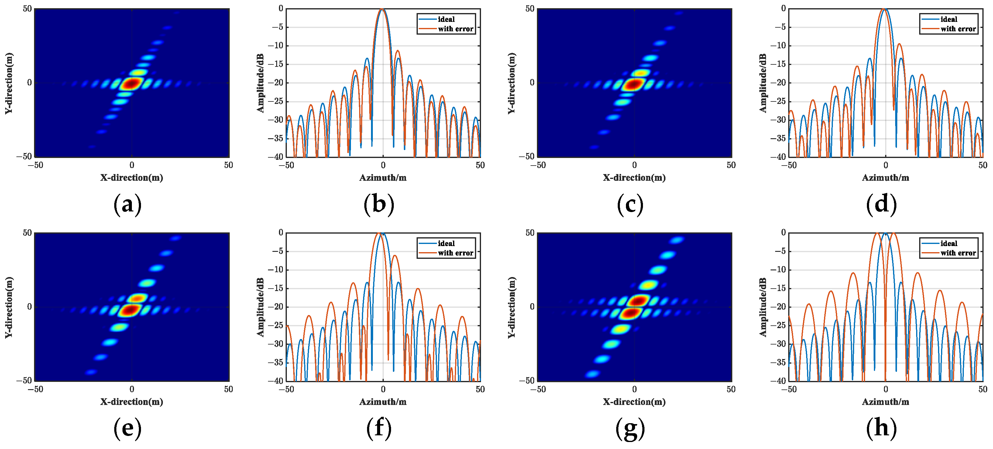
Figure 4a–c show BP images with frequency errors of Δ f n = ± 0.26   Hz , Δ f n = ± 0.5   Hz , and Δ f n = ± 1   Hz , respectively. The errors are set according to the rule that neighboring radars have the same absolute value and opposite signs of error, such as Δ f = { 0.26 , 0.26 , 0.26 , , 0.26 }   Hz . This rule maximizes the phase error between neighboring radars. Figure 4a compares their azimuth profiles with an ideal azimuth profile. We can see that as Δ f n increases, the sidelobes’ levels rise. When Δ f n = ± 0.26   Hz , meaning that the maximum phase error between neighboring echoes is exactly π / 4 , a clear elevation of the sidelobe level can be seen, but the effect on the imaging results is small. When Δ f n = ± 0.5   Hz , meaning that the maximum phase error between neighboring echoes is π / 2 , the sidelobes’ levels are so high that false targets begin to appear in the imaging results. When Δ f n = ± 1   Hz , which means the maximum phase error is π , the target point splits into two indistinguishable points, causing enormous damage to the imaging.
Figure 4d–f show BP images with frequency errors of Δ f n 0.5   Hz , Δ f n 1   Hz , and Δ f n 2   Hz , respectively. The error for each radar in the multi-monostatic system is a random value within a range, which is a more realistic situation. Figure 5b compares their azimuth profiles with an ideal azimuth profile. Note that the image deviation caused by the large frequency error is neglected for a better comparison of the azimuthal profiles. As the error limit increases, which means the frequency stability decreases, the sidelobe interference and the image degradation worsens. When Δ f n 2   Hz , multiple sidelobes’ levels are almost as high as the main lobe level that the real target cannot be distinguished.
In order to quantitatively evaluate the effect of the error, we calculated the Impulse Response Width (IRW), Peak Sidelobe Level Ratio (PSLR), and integrated sidelobe level ratio (ISLR) of the above imaging results, as shown in Table 4. As the frequency synchronization error increases, the deterioration of the performance parameters is significant.

3.2. Random Error

According to Equation (11), random error ϕ n e t caused by the oscillator noise can be written as
ϕ n e t = φ n t τ n d φ n t
The power spectral density function of the random error can be written as
S ϕ n f = exp j 2 π f τ n d 1 2 S φ n f   = 4 m 2 sin 2 π f τ n d S φ f   = 2 m 2 S φ f 1 cos 2 π f τ n d
For different SAR systems, the impact caused by phase noise mainly depends on the time delay. Figure 6 shows the power spectrum density functions of random phase noise for GEO SAR and LEO SAR (the time delay is τ d = 6.7 ms ). The shorter slant range of the LEO SAR system results in a smaller time delay, which in turn enables sin 2 π f τ n d to have a suppression effect on the low-frequency noise. As the orbital altitude increases, the time delay increases and the low-frequency suppression decreases. The expression of the spectrogram contains the cosine term, which varies periodically, and when f τ n d is sufficiently large, the spectrum will have the sidelobe.
Phase noise can be decomposed into linear phase, quadratic phase, and high-frequency phase, leading to azimuthal offset, main flap widening, and integrated sidelobe level ratio (ISLR) deterioration in the SAR image, respectively. The azimuthal offset is negligible for the system resolution. Main flap widening is quantified by analyzing the variance of the quadratic phase error (QPE) over synthetic aperture time, which can be calculated from [15,40]
σ φ e 2 2 = m 2 π T s 2 4 0 1 T s f 4 sin 2 π f τ n d S φ f d f
The contribution of high-frequency phase noise to the ISLR of an SAR image can be expressed as follows:
ISLR osc = 4 m 2 1 / T s sin 2 π f τ S φ f d f
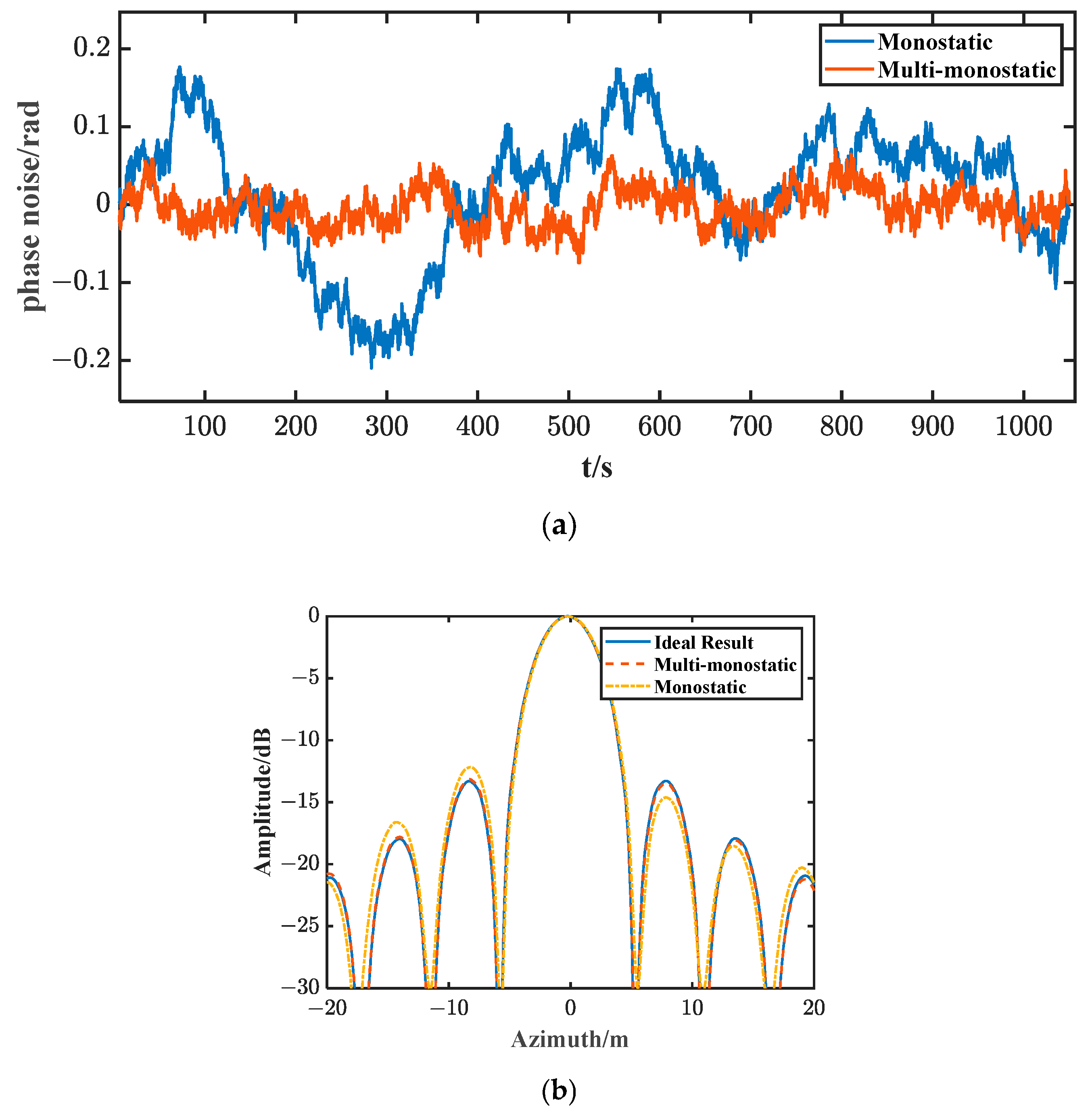
Figure 7a,b illustrate variation curves of the standard deviation of QPE and ISLR caused by high-frequency phase noise. In our multi-monostatic configuration, synthetic aperture time is reduced to 1 / N of the monostatic system for the same resolution requirement, which leads to a significant reduction in the influence of phase noise. According to the simulation parameters in Table 2 and Table 3, the synthetic aperture time of the multi-monostatic system is 105 s, where the corresponding QPE is 0.04 rad and the ISLR loss is −25 dB, while the synthetic aperture time of the monostatic system corresponds a QPE of 0.11 rad and an ISLR loss of −16 dB.
By designing filter whose frequency response agrees with the power spectrum density in Equation (23), the phase noise can be simulated in Figure 8a, where the phase noise of the multi-monostatic system is combined with the phase noise of each platform. Figure 8b shows the azimuth profiles with the two kinds of phase noise. As seen in Figure 8, the distributed system effectively shortens the work time, enabling smaller phase noise and less impact on imaging. Table 6 quantifies the performance metrics, showing it has lower PSLR and ISLR in the multi-monostatic system.

4. Autofocus Algorithm for Frequency Synchronization Error Compensation

The GEO SAR system exhibits completely different characteristics from LEO SAR and airborne SAR in terms of being affected by oscillator errors due to big time delay and long synthetic aperture time. The multi-monostatic configuration proposed in this paper is able to attenuate the effect of oscillator phase noise to some extent due to the reduction in the synthetic aperture time, but abrupt changes occur at the junctions of echoes between multiple channels. All these reasons make a higher demand on the stability of the frequency source.
In existing synchronization methods, direct signal synchronization requires additional electromagnetic wave signals to be transmitted and received between satellites, and dedicated synchronization link requires the design of additional hardware. Both of them put an extra burden on the system. Considering that frequency synchronization errors in this configuration eventually lead to phase errors, which can be estimated by many well-established algorithms, we proposed the autofocus back-projection (ABP) algorithm based on phase error estimation as a new synchronization method. The choice of autofocus algorithm is related to our imaging algorithm. Further, by analyzing specific error characteristics, we are able to incorporate a priori information to improve the ABP algorithm, making it significantly less computationally intensive while maintaining imaging performance.

4.1. Autofocus Back-Projection Algorithm

Considering the complexity of GEO SAR trajectories, we use the BP algorithm for imaging. We assume that b k is the back-projected value vector of the echo at the k -th azimuth sampling position to all grid points in the imaging scene, and ideally the BP algorithm imaging result is
z = k = 1 K b k
where K is the azimuth sampling number. In the presence of azimuthal phase error ϕ k , the imaging result is
z = k = 1 K b ˜ k = k = 1 K b k e j ϕ k
The autofocus back-projection (ABP) algorithm improves image quality by estimating the phase error in each azimuth sampling position and compensating back for it. Defining the estimated phase error as ϕ ^ = ϕ ^ 1 ϕ ^ k ϕ ^ K , we then have the image after phase error correction, as follows:
z ^ = k = 1 K b ˜ k e j ϕ ^ k
The sharpness value of an image is an important characterization quantity for detecting the degree of image focusing. There are various expression forms of sharpness, such as power sharpness, logarithmic sharpness, square sharpness, and so on, in which the square sharpness can be strengthened and weakened by approximate equal amplitude of the strong and weak targets of the image and has shown good characterization performance in different scenarios. The sharpness of the image is lower when the image is out of focus and corresponds to a higher sharpness value when the image is well focused [41]. Adopting the Maximizing Image Sharpness (MIS) rule, the objective function is given by
ϕ ^ = arg   max ϕ s ϕ
where s ϕ is the sharpness of the image, which is defined as the form s ϕ = i u i 2 , with u i = z i 2 = z i z i denoting the intensity of the i -th pixel.
Equation (29) is a multivariate optimization problem. By using the coordinate descent method, it can be reduced to a univariate optimization problem. The estimation of the k -th variable in the l -th iteration is
ϕ ^ k l = arg   max ϕ s ϕ ^ 1 l , , ϕ ^ k 1 l , ϕ , ϕ ^ k + 1 l 1 , , ϕ ^ K l 1
Substituting Equation (30) into Equation (28) yields
z ϕ = q = 1 k 1 b ˜ q e j ϕ ^ q l + q = k + 1 K b ˜ q e j ϕ ^ q l 1 + b ˜ k e j ϕ = x + e j ϕ y
where y is always the back-projected value corresponding to the current parameter to be estimated, and x is determined by the other back-projection values and phase errors. The update of x is the main step of the algorithm, as follows:
y = b ˜ k x k l = q = 2 K b ˜ q e j ϕ ^ q l 1 , k = 1 x k l = x k 1 l + b ˜ k 1 e j ϕ ^ k 1 l b ˜ k e j ϕ ^ k l 1 , k > 1
Equation (29) can be written as
ϕ ^ = arg   max ϕ i u i 2 = arg   max ϕ i z i z i 2
Based on the geometrical interpretation of the optimization model proposed by Ash, the optimal single-pulse phase corrections can be derived in closed form as the solution of a quartic polynomial [42]. The flow chart of the ABP algorithm is illustrated in Figure 9. The iteration termination condition is written as follows:
s ϕ l + 1 s ϕ l s ϕ l + 1 10 4
Assuming that the distributed system has a fixed frequency error of Δ f n 2 and random phase noise, the results of ABP are shown in Figure 10. Observing the true values in Figure 10a, it can be concluded that the phase error is mainly determined by the fixed frequency error, and the random phase noise is very small, so the phase error between the multi-monostatic platforms is segmented, where abrupt changes occur at the data connections between different platforms. The defocusing of the image is mainly determined by the mutation errors at these junctions, so the key to focusing the image is to correctly estimate the value of the phase error at the connections.
Observing Figure 10a, the phase error obtained by ABP does not exactly match the actual error, but good focusing results are still obtained. This is due to the fact that the ABP algorithm correctly estimates the constant phase error, i.e., the abrupt change error between segments, as shown in Figure 10b. After compensating for the mutation errors, the remaining estimation error varies linearly, which only causes an azimuthal shift of the image and does not affect the focusing result. Figure 11 gives the imaging result of ABP and the result of compensation using only the node errors. We can see that Figure 11a has an azimuthal offset, whereas Figure 11b does not.
The variations in image sharpness value and mean square error (MSE) with the number of iterations are shown in Figure 11. The sharpness value improves dramatically after the first iteration, and the MSE is already less than 5 × 10 5 . After the subsequent iterations, the sharpness value of the image reaches the true value, and the mean square error is less than 2 × 10 5 . Combining Figure 12, the first iteration achieved a better result, and the last three iterations have essentially the same results.

4.2. Node Autofocus Back-Projection Algorithm

ABP algorithm uses all information of the whole scene to calculate the sharpness, so it needs to compute and store the back-projected values for all azimuth samples, which results in a heavy burden for memory. Assume that the number of discrete cells per dimension in the imaging scene is M and the total number of azimuth samples is K , the required memory to store the back-projections is (in double precision) [43]
M p = 8 × M 2 × K
As the scene size and the number of azimuth samples increase, the required memory increases dramatically, which limits ABP’s practical application.
According to our previous analysis, the phase error due to the frequency synchronization error is segmented. The phase errors between the echoes are small within each segment, and the key to focusing the image is to correctly estimate the phase error at the connections between several platforms. Therefore, when using ABP, the focus should be on the estimation of the connections, and the error within the segment can be ignored to some extent.
Based on the above analysis, we propose the Node ABP (NABP) algorithm. There are two key steps in the algorithm: estimate and update. First, we estimate the phase error at the head position for each segment, and second, we update the phase error values at the other locations within the segment to be consistent with the head. The schematic diagram of NABP is shown in Figure 13. The flow chart of the program in Figure 8 can be changed to Figure 14, where an additional judgment statement is added.
The specific calculations are analyzed next. According to Equation (28), the BP imaging result of the multi-monostatic system can be rewritten as
z = n k n b ˜ k n = n exp j Φ n k n b k n
where n = 1 , , N is the platform number, and k n refers to the azimuth echoes captured by the n -th SAR. The estimated phase error is Φ ^ = Φ ^ 1 Φ ^ i Φ ^ N .
According to Equations (31) and (32), it is no longer necessary to update each x , but only the x at the head and the end of the segment. In the l -th iteration, the x of the n -th segment head can be written as
x n _ h e a d l = x n _ h e a d 1 l + b ˜ n _ h e a d 1 e j ϕ ^ n _ h e a d 1 l b ˜ n _ h e a d e j ϕ ^ n _ h e a d l 1   = x n 1 _ e n d l + b ˜ n 1 _ e n d e j Φ ^ n 1 l b ˜ n _ h e a d e j Φ ^ n l 1
It is easy to understand that the previous back-projected value of the n -th segment head is the n 1 -th segment end, and the x of the n -th segment end can be written as
x n _ e n d l = x n _ h e a d l + b ˜ n _ h e a d + b ˜ n _ 2 + + b ˜ n _ e n d 1 e j Φ ^ n l b ˜ n _ 2 + b ˜ n _ 3 + + b ˜ n _ e n d e j Φ ^ n l 1   = x n _ h e a d l + B n b ˜ n _ e n d e j Φ ^ n l B n b ˜ n _ h e a d e j Φ ^ n l 1
where B n = n _ h e a d n _ e n d b ˜ n is the back-projection sum of the n -th segment.
With the above analysis, for the n -th segment, we only need to store the first back-projected value b ˜ n _ h e a d , the last back-projected value b ˜ n _ e n d , and the sum of the back-projected values B n for x update and phase error estimation. When there are N radars operating simultaneously in the system, only 3 N back-projected values need to be stored, which is much less than the total number of azimuth samples K . For ABP processing, there are K parameters to be estimated, meaning that the estimation operation is performed K times in one iteration. Suppose l A B P is the number of iterations in which the ABP reaches the threshold value, then the estimation operation is performed a total of l A B P K times. For NABP processing, there are N parameters to be estimated. The estimation operation is performed a total of l N A B P N times where l N A B P is the number of iterations in which the NABP reaches the threshold value. l A B P and l N A B P are generally not that significantly different, while K is more than three orders of magnitude larger than N . In this way, NABP requires much less memory and computation to estimate the phase error due to frequency synchronization errors. The differences in computational complexity and required storage between the proposed NABP and ABP are given in Table 7.
Some simulations are conducted to verify the ability of the NABP algorithm we proposed. The ABP algorithm takes 4 iterations to reach the iteration termination condition, while the NABP algorithm requires 31 iterations. The variation in sharpness values with the number of iterations is plotted in Figure 15. We find that the sharpness values using the NABP algorithm grow slowly, so more iterations are needed to achieve a similar effect with the ABP algorithm. Although the iteration condition is not reached, the sharpness values after 15 iterations are not far from the true values.
The comparisons of azimuth profiles are shown in Figure 16. There are azimuth profiles of results after 4 iterations using ABP, after 4 iterations using NABP, after 15 iterations using NABP, and after 31 iterations using NABP. Enlarging the left and right first sidelobes, we find only a small difference there. In fact, even with 31 iterations, the amount of computation and storage of NABP is still much smaller than that of ABP; thus, it is an effective way to improve computational efficiency in terms of performing frequency synchronization error compensation. Target imaging performance in different cases is given in Table 8.

5. Conclusions

In this paper, we discussed fully the frequency synchronization problem of multi-monostatic configuration. It is pointed out that due to the high orbital characteristics and long synthetic aperture time, the fixed frequency errors lead to a constant phase error in the echoes block of each monostatic radar, which destroys the coherence between the echoes blocks and thus leads to image scattering when multi-monostatic configurations are imaged cooperatively. To ensure that the phase error between neighboring echoes is less than π / 4 , it is necessary to ensure that the frequency deviation of the frequency source is less than 0.26 Hz during the synthetic aperture time, i.e., the stability of the frequency source is y ¯ T s 2.1 × 10 10 . We also discuss the effect of phase noise on the cooperative imaging of multi-monostatic configurations and show that the characteristics of high orbits and long synthetic aperture times make the effect of phase noise on GEO SAR larger than that on LEO SAR and that the quadratic phase error due to phase noise can be 0.11 rad over the synthetic aperture time of 1050 s, with an ISLR loss of −16 dB. Multi-monostatic configuration is able to reduce the synthetic aperture time, thus attenuating the effect of phase noise on imaging. Overall, the effect of frequency synchronization errors on multi-monostatic configurations is mainly caused by fixed frequency errors of each radar, which result in a constant phase error for each echoes block. Clarifying this point is conducive to the subsequent estimation and compensation of the phase error.
To solve the phase error caused by frequency synchronization error, we proposed the ABP algorithm, and experimental data verified the effectiveness of the proposed algorithm. Analyzing the estimation results of ABP, we found that only the estimations at the connection position of different radars are significant. Based on the priori knowledge, we proposed the NABP algorithm that only estimates the phase errors at the nodes utilizing the ABP algorithm, which can basically maintain the estimation performance while greatly reducing the memory burden and time consumption and can effectively solve the frequency synchronization problem under this configuration. With our simulation parameters, NABP reduced at least 50–100 times the amount of data storage and computation compared to ABP.

Author Contributions

Conceptualization, X.S. and L.C.; methodology, X.S., L.C. and Z.Z.; software, X.S., Z.Z. and H.D.; supervision, L.C. and X.H.; validation, X.S. and L.C.; writing—original draft, X.S. and H.D.; writing—review and editing, X.S., L.C. and X.H. All authors have read and agreed to the published version of the manuscript.

Funding

This research was funded by National Natural Science Foundation of China grant number 62101566.

Data Availability Statement

No new data were created or analyzed in this study. Data sharing is not applicable to this article.

Conflicts of Interest

The authors declare no conflicts of interest.

References

  1. Long, T.; Hu, C.; Ding, Z.; Dong, X.; Tian, W.; Zeng, T. Geosynchronous SAR: System and Signal Processing; Springer: Singapore, 2018. [Google Scholar]
  2. Zhang, W.; Yang, S.; Fan, Y.; Wu, W.; Zhao, B. Application potential and working mode requirements of GEO SAR satellite for comprehensive disaster reduction. Spacecr. Eng. 2017, 26, 127–131. [Google Scholar]
  3. Tomiyasu, K.; Pacelli, J.L. Synthetic Aperture Radar Imaging from an Inclined Geosynchronous Orbit. IEEE Trans. Geosci. Remote Sens. 1983, GE-21, 324–329. [Google Scholar] [CrossRef]
  4. Hobbs, S.E.; Bruno, D. Radar imaging from geosynchronous orbit: Temporal decorrelation aspects. IEEE Trans. Geosci. Remote Sensing. 2010, 48, 2924–2929. [Google Scholar]
  5. Hu, C.; Chen, Z.; Li, Y.; Dong, X.; Hobbs, S. Research progress on geosynchronous synthetic aperture radar. Fundam. Res. 2021, 1, 346–363. [Google Scholar] [CrossRef]
  6. Guarnieri, A.M.; Tebaldini, S.; Rocca, F.; Broquetas, A. GEMINI: Geosynchronous SAR for Earth monitoring by interferometry and imaging. In Proceedings of the IEEE International Geoscience and Remote Sensing Symposium, Munich, Germany, 22–27 July 2012. [Google Scholar]
  7. Guarnieri, A.G.A.M.; Broquetas, A.B.A.; Recchia, A.R.A.; Rocca, F.R.F.; Ruiz-Rodon, J.R.J. Advanced Radar Geosynchronous Observation System: ARGOS. IEEE Geosci. Remote Sens. Lett. 2015, 12, 1406–1410. [Google Scholar] [CrossRef]
  8. Dong, X.; Hu, C.; Chen, Z. Formation design and performance analysis for distributed geosynchronous SAR. J. Nanjing Univ. Inf. Sci. Technol. (Nat. Sci. Ed.) 2020, 12, 236–245. [Google Scholar]
  9. Liang, D.; Zhang, H.; Liu, K.; Liu, D.; Wang, R.Y. Phase Synchronization Techniques for Bistatic and Multistatic Synthetic Aperture Radar: Accounting for Frequency Offset. IEEE Geosci. Remote Sens. Mag. 2022, 10, 2–17. [Google Scholar] [CrossRef]
  10. Weiss, M. Time and Frequency Synchronisation Aspects for Bistatic SAR Systems. In Proceedings of the 5th European Conference on Synthetic Aperture Radar (EUSAR 2004), Ulm, Germany, 25–27 May 2004; Volume 1. [Google Scholar]
  11. Fang, Z.; Li, Z.; Mao, X.; Yang, Y.; Wu, J.; Yang, J. A Time-Domain Image Formation for High Frame Rate UAV Swarm SAR. In Proceedings of the IGARSS 2022—2022 IEEE International Geoscience and Remote Sensing Symposium, Kuala Lumpur, Malaysia, 17–22 July 2022. [Google Scholar]
  12. Sun, X.; Chen, L.; Huang, X. Impact Analysis and Compensation Method of Frequency Synchronization Error in Distributed SAR. In Proceedings of the 2023 8th International Conference on Signal and Image Processing (ICSIP), Wuxi, China, 8–10 July 2023. [Google Scholar]
  13. Wang, Y.; Ding, Z.; Li, L.; Liu, M.; Ma, X.; Sun, Y.; Zeng, T.; Long, T. First Demonstration of Single-Pass Distributed SAR Tomographic Imaging With a P-Band UAV SAR Prototype. IEEE Trans. Geosci. Remote Sens. 2022, 60, 5238618. [Google Scholar] [CrossRef]
  14. Auterman, J.L. Phase-Stability Requirements for A Bistatic Sar. Microw. Rf. 1984, 23, 48. [Google Scholar]
  15. Krieger, G.; Younis, M. Impact of oscillator noise in bistatic and multistatic SAR. IEEE Geosci. Remote Sens. Lett. 2006, 3, 424–428. [Google Scholar] [CrossRef]
  16. Wang, W. Clock timing jitter analysis and compensation for bistatic synthetic aperture radar systems. Fluct. Noise Lett. 2007, 7, L341–L350. [Google Scholar] [CrossRef]
  17. Wang, W.Q.; Ding, C.B.; Liang, X.D. Time and phase synchronisation via direct-path signal for bistatic synthetic aperture radar systems. IET Radar Sonar Navig. 2008, 2, 1–11. [Google Scholar] [CrossRef]
  18. Dong, Z.; Liang, D.; Zhang, Y. Analysis of frequency synchronization error in spaceborne parasitic SAR system. Guofang Keji Daxue Xuebao/J. Natl. Univ. Def. Technol. 2006, 28, 85. [Google Scholar]
  19. Rodriguez-Cassola, M.; Baumgartner, S.V.; Krieger, G. Bistatic TerraSAR-X/F-SAR spaceborne-airborne SAR experiment: Description, data processing, and results. IEEE Trans. Geosci. Remote Sens. 2010, 48, 781–794. [Google Scholar] [CrossRef]
  20. Espeter, T.; Walterscheid, I.; Klare, J.; Gierull, C.; Brenner, A.; Ender, J.; Loffeld, O. Progress of Hybrid Bistatic SAR:Synchronization Experiments and First Imaging Results. In Proceedings of the 7th European Conference on Synthetic Aperture Radar, Friedrichshafen, Germany, 2–5 June 2008. [Google Scholar]
  21. Zhang, H.; Deng, Y.; Wang, R.; Li, N.; Zhao, S.; Hong, F.; Wu, L.; Loffeld, O. Spaceborne/Stationary Bistatic SAR Imaging with TerraSAR-X as an Illuminator in Staring-Spotlight Mode. IEEE Trans. Geosci. Remote Sens. 2016, 54, 5203–5216. [Google Scholar] [CrossRef]
  22. Cassola, M.R.; Martone, M.; De Zan, F.; Lopez-Dekker, P.; Prats, P.; Braeutigam, B.; Baumgartner, S.; Schulze, D.; Hajnsek, I.; Younis, M.; et al. TanDEM-X: A radar interferometer with two formation-flying satellites. Acta Astronaut. 2013, 89, 83–98. [Google Scholar]
  23. Younis, M.; Metzig, R.; Krieger, G. Performance prediction of a phase synchronization link for bistatic SAR. IEEE Geosci. Remote Sens. Lett. 2006, 3, 429–433. [Google Scholar] [CrossRef]
  24. Rodriguez-Cassola, M.; Prats-Iraola, P.; López-Dekker, P.; Reigber, A.; Krieger, G.; Moreira, A. Autonomous time and phase calibration of spaceborne bistatic SAR systems. In Proceedings of the EUSAR 2014: 10th European Conference on Synthetic Aperture Radar, Berlin, Germany, 2–6 June 2014. [Google Scholar]
  25. D’Errico, E.B.M. Distributed Space Missions for Earth System Monitoring; Springer Science & Business Media: Berlin, Germany, 2013. [Google Scholar]
  26. Xie, Z.; Xu, Z.; Fan, C.; Han, S.; Huang, X. Robust Radar Waveform Optimization Under Target Interpulse Fluctuation and Practical Constraints Via Sequential Lagrange Dual Approximation. IEEE Trans. Aerosp. Electron. Syst. 2023, 59, 9711–9721. [Google Scholar] [CrossRef]
  27. Zeng, T.; Long, T.; Liu, Z.; Hu, C.; Liu, F. The Accurate Focusing and Resolution Analysis Method in Geosynchronous SAR. IEEE Trans. Geosci. Remote Sens. 2011, 49, 3548–3563. [Google Scholar]
  28. Liu, Y.; Li, Z.; Suo, Z.; Li, J.; Bao, Z. Impact of frequency oscillator errors on GEO SAR imaging performance. Syst. Eng. Electron. 2015, 37, 61–66. [Google Scholar]
  29. He, Z.; He, F.; Sun, Z.; Dong, Z. Analysis of oscillator stability index in geosynchronous SAR. Bull. Surv. Mapp. 2014, 4, 19–21. [Google Scholar]
  30. Yarman, C.E.; Yazici, B.; Cheney, M. Bistatic synthetic aperture radar imaging for arbitrary flight trajectories. IEEE Trans. Image Process. 2008, 17, 84–93. [Google Scholar] [CrossRef]
  31. Schulz, T.J. Optimal Sharpness Function for SAR Autofocus. IEEE Signal Process. Lett. 2007, 14, 27–30. [Google Scholar] [CrossRef]
  32. Fienup, J.R.; Miller, J.J. Aberration correction by maximizing generalized sharpness metrics. J. Opt. Soc. Am. A (Opt. Image Sci. Vis.) 2003, 20, 609–620. [Google Scholar] [CrossRef]
  33. Chen, L.; An, D.; Huang, X. Extended Autofocus Backprojection Algorithm for Low-Frequency SAR Imaging. IEEE Geosci. Remote Sens. Lett. 2017, 14, 1323–1327. [Google Scholar] [CrossRef]
  34. Rutman, J.; Walls, F.L. Characterization of frequency stability in precision frequency sources. Proc. IEEE 1991, 79, 952–960. [Google Scholar] [CrossRef]
  35. Rutman, J. Characterization of phase and frequency instabilities in precision frequency sources 15th years of progress. Proc. IEEE 1978, 66, 1048–1075. [Google Scholar] [CrossRef]
  36. Zhou, P. System Design and Synchronization Technique of Spaceborne/Airborne Hybrid Bistatic Synthetic Aperture Radar; University of Electronic Science and Technology of China: Chengdu, China, 2008. [Google Scholar]
  37. Wang, Y.; Qu, C.; Gao, Y. Influence of Linear Phase error to image Quality for FMCW SAR. Microcomput. Inf. 2009, 25, 285–287. [Google Scholar]
  38. Wang, Y.; Qu, C. Influence of Secondary Phase Error to Image Quality for FMCW SAR. Command Control Simul. 2009, 31, 104–106. [Google Scholar]
  39. Du, H.; Song, Y.; Jiang, N.; An, D.; Wang, W.; Fan, C.; Huang, X. A Novel SAR Ground Maneuvering Target Imaging Method Based on Adaptive Phase Tracking. IEEE Trans. Geosci. Remote Sens. 2023, 61, 5211916. [Google Scholar] [CrossRef]
  40. Xie, X.; Pi, Y. Impact and estimation of frequency source noise on bistatic SAR. J. Syst. Eng. Electron. 2010, 32, 275–278. [Google Scholar]
  41. Gao, Y.; Yu, W. A SAR Back Projection Autofocusing Algorithm Based on Legendre Approximation. J. Radars 2014, 3, 176–182. [Google Scholar] [CrossRef]
  42. Ash, J.N. An Autofocus Method for Backprojection Imagery in Synthetic Aperture Radar. IEEE Geosci. Remote Sens. Lett. 2012, 9, 104–108. [Google Scholar] [CrossRef]
  43. Hu, K.; Zhang, X.; He, S.; Zhao, H.; Shi, J. A Less-Memory and High-Efficiency Autofocus Back Projection Algorithm for SAR Imaging. IEEE Geosci. Remote Sens. Lett. 2015, 12, 890–894. [Google Scholar]
Figure 1. Typical power spectral density function of the spaceborne SAR system.
Remotesensing 16 01470 g001
Figure 2. Distributed configuration of GEO SAR system.
Remotesensing 16 01470 g002
Figure 3. Results of bi-monostatic GEO SAR with various frequency errors: (a) BP image with Δ f = π / 8 . (b) Azimuth profile of (a). (c) BP image with Δ f = π / 4 . (d) Azimuth profile of (c). (e) BP image with Δ f = π / 2 . (f) Azimuth profile of (e). (g) BP image with Δ f = π . (h) Azimuth profile of (g).
Remotesensing 16 01470 g003
Figure 4. BP images of multi-monostatic GEO SARs with various frequency errors: (a) Δ f n = ± 0.26   Hz ; (b) Δ f n = ± 0.5   Hz ; (c) Δ f n = ± 1   Hz ; (d) Δ f n 0.5   Hz ; (e) Δ f n 1   Hz ; and (f) Δ f n 2   Hz .
Remotesensing 16 01470 g004
Figure 5. Azimuth profiles of multi-monostatic GEO SARs with various frequency errors. (a) Given frequency errors. (b) Random frequency errors.
Remotesensing 16 01470 g005
Figure 6. The power spectrum density functions of random phase noise for GEO SAR and LEO SAR.
Remotesensing 16 01470 g006
Figure 7. Influence of phase noise with synthetic aperture time. (a) Standard deviation of QPE varies with synthetic aperture time. (b) ISLR caused by high-frequency phase noise varies with synthetic aperture time.
Remotesensing 16 01470 g007
Figure 8. Influence of phase noise in monostatic and multi-monostatic GEO SAR system. (a) Phase noise in monostatic and multi-monostatic GEO SAR system. (b) The azimuth profiles with the two kinds of phase noise.
Remotesensing 16 01470 g008
Figure 9. Flow chart of the ABP algorithm.
Remotesensing 16 01470 g009
Figure 10. Results of ABP. (a) Estimations of azimuth samples. (b) Estimations of azimuth node samples. (c) The azimuth profiles after ABP processing.
Remotesensing 16 01470 g010
Figure 11. Results of ABP. (a) Result after ABP processing. (b) Result after node error compensation.
Remotesensing 16 01470 g011
Figure 12. Sharpness and estimation MSE after ABP. (a) Sharpness after ABP; (b) estimation MSE after ABP.
Remotesensing 16 01470 g012
Figure 13. Schematic diagram of the NABP algorithm.
Remotesensing 16 01470 g013
Figure 14. Flow chart of the NABP algorithm.
Remotesensing 16 01470 g014
Figure 15. The variation in sharpness values with the number of iterations.
Remotesensing 16 01470 g015
Figure 16. The azimuth profiles in different cases.
Remotesensing 16 01470 g016
Table 1. Typical coefficients of the oscillators.
ParametersValues
a / dB −95
b / dB −90
c / dB −200
d / dB −130
e / dB −155
Table 2. Typical orbital elements for GEO SAR system.
ParametersValues
Semi-major axis42,164 km
Eccentricity0
Inclination 16 °
Argument of periapsis 90 °
Right ascension of the ascending node 0 °
True anomaly 0 °
Table 3. Key parameters for analysis and simulation.
ParametersValues
f 0 : Center frequency 1.25   GHz
B : Signal frequency bandwidth 60   MHz
P R F : Pulse repetition frequency 10   Hz
T p : Pulse width 250   μ s
N : Number of radars 10
T s : Synthetic aperture time 105   s
Table 4. Target imaging performance with fixed frequency offset in the bi-monostatic GEO SAR.
ΔfΔφIRW (m)PSLR (dB)ISLR (dB)Shift (m)
004.98−13.31−10.310
0.256 π / 8 5.02−11.17−9.83−0.45
0.512 π / 4 4.98−9.41−8.61−1.06
1.024 π / 2 4.90−6.06−5.39−2.12
2.048 π 4.5 (13.11)−0.010.91−4.22
Table 5. Target imaging performance with fixed frequency offset.
Δ f n (Hz)IRW (m)PSLR (dB)ISLR (dB)
04.98−13.28−10.35
± 0.26 5.00−10.68−6.15
± 0.5 4.92−4.36−0.59
± 1.0 4.97−0.04/
Δ f n 0.5   5.16−7.49−4.94
Δ f n 1 4.80−5.270.97
Δ f n 2 5.17−1.403.23
Table 6. Target imaging performance with random phase noise.
IRW (m)PSLR (dB)ISLR (dB)
Ideal results4.98−13.28−10.35
Multi-monostatic5.00−13.13−10.34
Monostatic4.98−12.17−10.06
Table 7. Comparison of ABP and NABP in terms of computational complexity and storage.
ABPNABP
Estimated Parameter K N
Computational Complexity l A B P K l N A B P N
Storage 8 M 2 K 8 M 2 3 N
Table 8. Target imaging performance in different cases.
IRW (m)PSLR (dB)ISLR (dB)
04.98−13.28−10.35
ABP,45.00−13.32−10.37
NABP,45.00−12.00−10.17
NABP,155.00−12.86−10.32
NABP,315.00−13.18−10.33
Disclaimer/Publisher’s Note: The statements, opinions and data contained in all publications are solely those of the individual author(s) and contributor(s) and not of MDPI and/or the editor(s). MDPI and/or the editor(s) disclaim responsibility for any injury to people or property resulting from any ideas, methods, instructions or products referred to in the content.

