Article

Toward a More Robust Estimation of Forest Biomass Carbon Stock and Carbon Sink in Mountainous Region: A Case Study in Tibet, China

1
State Key Laboratory of Tibetan Plateau Earth System, Resources and Environment (TPESRE), Institute of Tibetan Plateau Research, Chinese Academy of Sciences, Beijing 100101, China
2
University of Chinese Academy of Sciences, Beijing 100101, China
3
Department of Computer Science and Technology, Tsinghua University, Beijing 100084, China
4
College of Ecology, Lanzhou University, Lanzhou 730000, China
5
College of Geography and Ocean Sciences, Yanbian University, Yanji 133002, China
6
School of Geospatial Engineering and Science, Sun Yat-sen University, Zhuhai 519082, China
*
Author to whom correspondence should be addressed.
Remote Sens. 2024, 16(9), 1481; https://doi.org/10.3390/rs16091481
Submission received: 31 March 2024 / Revised: 16 April 2024 / Accepted: 20 April 2024 / Published: 23 April 2024

Abstract

:
Mountainous forests are pivotal in the global carbon cycle, serving as substantial reservoirs and sinks of carbon. However, generating a reliable estimate remains a considerable challenge, primarily due to the lack of representative in situ measurements and proper methods capable of addressing their complex spatial variation. Here, we proposed a deep learning-based method that combines Residual convolutional neural networks (ResNet) with in situ measurements, microwave (Sentinel-1 and VOD), and optical data (Sentinel-2 and Landsat) to estimate forest biomass and track its change over the mountainous regions. Our approach, integrating in situ measurements across representative elevations with multi-source remote sensing images, significantly improves the accuracy of biomass estimation in Tibet’s complex mountainous forests (R2 = 0.80, root mean squared error = 15.8 MgC ha−1). Moreover, ResNet, which addresses the vanishing gradient problem in deep neural networks by introducing skip connections, enables the extraction of complex spatial patterns from limited datasets, outperforming traditional optical-based or pixel-based methods. The mean value of forest biomass was estimated as 162.8 ± 21.3 MgC ha−1, notably higher than that of forests at comparable latitudes or flat regions in China. Additionally, our findings revealed a substantial forest biomass carbon sink of 3.35 TgC year−1 during 2015–2020, which is largely underestimated by previous estimates, mainly due to the underestimation of mountainous carbon stock. The significant carbon density, combined with the underestimated carbon sink in mountainous regions, emphasizes the urgent need to reassess mountain forests to better approximate the global carbon budget.

1. Introduction

Mountainous forests, spanning extensive territories, are pivotal in the sequestration of atmospheric carbon [1]. Refining our estimates of carbon reservoirs within these biomes is crucial for climate change mitigation strategies and to inform sustainable forestry [2,3,4,5]. Nonetheless, the diverse forest types, challenging topography, and heterogeneous climate of mountain regions impose significant difficulties in calculating forest biomass and carbon sequestration rates [6,7]. Across the elevational gradient, forest types transition from broadleaf to mixed, and then to coniferous forests and eventually an alpine tree line, which occurred over short horizontal spans, and paralleled by varied biomass. Marked biomass differences also persist between sunlit and shaded slopes in mountain regions. Traditional assessment methods could not capture the intricate spatiotemporal dynamics of mountain forests, hindered by limited in situ measurements and methods suitable for their complex spatial variations [8]. Consequently, accurate biomass and carbon sequestration estimates for mountainous terrain remained challenging [9].
First, in situ measurements in mountainous areas were limited, as monitoring sites often were unevenly distributed and too few to accurately reflect the complex spatial variations, especially across large elevational gradients. Such insufficiency compromised the accuracy of forest carbon stock assessments and their variation within these complex landscapes. For example, a widely used forest biomass inventory dataset for Eurasia [10] included only 30.6% of measurements from mountain regions as defined by the Global Mountain Biodiversity Assessment (GMBA) datasets [11], and included only 19.9% of measurements which were located in rugged regions with slopes greater than 10°. This deficiency was more pronounced across China, where only 6.45% of measurements were located in mountain regions with an elevation higher than 1000 m. Therefore, there was an emergent need to conduct widespread measurements over mountain regions [12,13]. However, the remoteness and access difficulties in mountainous regions made extensive field surveys challenging, often precluding the collection of widespread observational data [14,15]. Thus, determining whether representative sampling along elevational gradients could enable efficient monitoring and enhance forest biomass estimations emerged as a primary issue to address.
Second, forest biomass carbon stock and sink estimations had increasingly relied on remote sensing data, ranging from optical images (e.g., Landsat, Sentinel-2, IKONOS, QuickBird) to SAR (e.g., Sentinel-1, SSDD, ALOS-2) and VOD (e.g., L-VOD, X-VOD, P-VOD) datasets, each offering unique insights into vegetation structure [16,17,18]. However, how to effectively combine multi-source remote sensing data remained to be solved. Specifically, optical remote sensing imagery provided spectral reflectance of the forest canopy, enabling the acquisition of features related to the forest’s top canopy, notably leaves [19,20]. However, it fell short in detecting the structural components of trunks and branches, resulting in potential bias in forest carbon estimations [21]. Advanced remote sensing techniques such as LiDAR [22,23] and microwave remote sensing [24,25] could effectively penetrate the forest canopy, provide forest structure for biomass analysis, and were less susceptible to weather conditions [26]. For example, C-band SAR data provided by Sentinel-1A/B satellites aboard the ESA (European Space Agency) had been consistently providing valuable data on forest vertical structure through multiple polarization modes since 2014 [27,28]. There have been studies showing the proficiency of SAR data in regional biomass studies [29,30], yet the penetration power of SAR has limitations in dense or high-biomass forests where it might underestimate biomass [31]. The L-band vegetation optical depth (L-VOD), which correlates with aboveground biomass carbon and water content within vegetation, had been extensively utilized as a proxy for vegetation biomass to monitor changes in carbon stocks [32,33]. VOD data, notably sensitive to woody biomass and non-saturating at high levels due to low-frequency microwaves [34], offered an effective biomass proxy. For instance, Fan et al. [35] detected changes in terrestrial tropical carbon stocks using L-VOD and found that the tropics were roughly carbon neutral during 2010–2017. Wigneron et al. [36] further showed that tropical forest biomass was a carbon source during the strong 2015–2016 El Niño event and did not recover to the pre-event level. While methods utilizing L-VOD were constrained by the assumption that the plant water-holding capacity remained constant. This assumption could potentially be challenged by climate variations and the physiological responses of vegetation [37,38,39]. Therefore, how to effectively combine the multi-source remote sensing data that reflect the multi-dimensional forest structure and attributes to accurately quantify forest biomass remained an unresolved issue.
Third, traditional methods that upscaled in situ measurements to regional wall-to-wall maps failed to capture the detailed spatial variations present in mountainous terrain. Such methods often employed pixel-based modeling, which neglected neighboring pixel information, including textural patterns crucial for depicting spatial variation [40,41]. However, with advancements in deep learning, particularly Convolutional Neural Networks (CNNs), these methods showed promise in overcoming various geospatial challenges, as evidenced by numerous researchers [42,43,44]. Unlike traditional pixel-based approaches that formed predictions from isolated pixels, CNNs leveraged the spatial context by considering information from neighboring pixels, thus offering a more complex representation of forest biomass distribution [45]. Integrating CNNs with multi-source remote sensing data, which provided insights into different forest components such as leaves, branches, and trunks, held the potential to significantly improve the mapping of regional biomass and carbon sinks.
Forests in Tibet, characterized by intact and natural state [45,46,47], potentially hold considerable carbon stock and serve as substantial carbon sinks. The elevation of forest over Tibet ranges from 8 to 4900 m. The rugged and complex terrain poses challenges for traditional methods of estimating biomass in mountainous forests, making it an ideal case study for our research. Hence, our objective is to devise a robust methodology for estimating forest biomass and biomass carbon sink, with a particular focus on mountainous forests, exemplified by those in the mountain regions of Tibet. Our research aimed to answer the following key questions: (1) whether representative in situ measurements along elevation could improve mountain forest biomass. (2) Do multi-source remote sensing data outperform single source results? (3) Whether the patch-based deep learning method outperforms the traditional pixel-based method in mountain forest biomass and carbon sink estimation. (4) The size of forest biomass carbon stock and carbon sequestration rate over Tibet.

2. Data Collection

2.1. Study Area

The Tibet Autonomous, situated in southwestern China, boasts a significant altitude range. This considerable variation in altitude harbors diverse climate types across Tibet [48], facilitating the growth of plants ranging from subtropical to boreal species. Consequently, Tibet harbors a forest ecosystem of exceptional biodiversity, earning recognition as one of China’s three major forested regions [46]. Forest distribution in Tibet is predominantly concentrated in the mountains and valleys of the Himalayas and the Hengduan Mountains in the southeast. Noteworthy is the Nyingchi Prefecture, home to China’s largest primeval forest area and revered as one of the most representative regions for global biodiversity.

2.2. Forest Inventory Data

We conducted in situ measurements (N = 67, red dots in Figure 1) during 2019 and 2023 with a special focus on the elevational gradient. Here, we set the elevation intervals as 100 m, ensuring that at least one sample was collected every 100 m from 33 m (a.s.l.) to 4500 m (a.s.l.). Each plot was set as a square of 10 × 10 m. We then measured the diameter at breast height (DBH), and height of each tree (DBH > 5 cm) and also recorded tree types. The forest aboveground biomass was obtained using the allometric model of each tree type. The average biomass of these sample points is 135.4 MgC ha−1, with an average elevation of 4673.4 m. In addition, we compiled data documented in the literature (N = 98, blue dots in Figure 1). Data should be measured near or after the year 2015, and satisfy the following two criteria (1) the inventory should be conducted at the plot scale rather than at the individual tree level [49]; (2) data should be collected from stable sites with no recent fires or human disturbances, verified through high-resolution imagery on Google Earth (interpreted manually from Google Earth high-resolution images). Data recorded only forest aboveground biomass was transformed into biomass by the shoot-to-root ratio of 0.35, following Liu et al. [8]. The distribution of inventory data which met those criteria is shown in Figure 1. However, the observation data were obtained between 2015 and 2023, while our analysis focused on the period from 2015 to 2020. This temporal mismatch could potentially introduce uncertainties in our estimation.

2.3. Microwave Remote Sensing Images

The Sentinel-1 data offer backscatter information in the Interferometric Wide Swath (IW) mode, capturing both VV (Vertical transmit–Vertical receive) and VH (Vertical transmit–Horizontal receive) polarizations at a spatial resolution of 10 m. We acquired median value data spanning the growing seasons (May to September) in 2015 and 2020 using the Google Earth Engine (GEE) platform [50] (https://earthengine.google.org/, accessed on 10 January 2024). These datasets underwent meticulous pre-processing, including noise elimination, terrain correction, and radiometric calibration, to ensure accuracy and reliability.
The vegetation optical depth (VOD) data were from the SMOS-ICV2-RE06 L-VOD product (L-VOD), which provides monthly VOD data at different microwave band frequencies since 2010. The VOD measured at microwave frequencies is related to the vegetation water content. And the vegetation water content can be related to the biomass and to its moisture status, which can be parameterized by the gravimetric moisture content Mg (%). The VOD data we utilized also originate from both the 2015 and 2020 periods, and we downscaled L-VOD data to 10 m resolution by linear spatial interpolation.

2.4. Optical Remote Sensing Image

We also obtained top-of-atmosphere reflectance data from Sentinel-2 level 2A and Landsat 8 images during the growing seasons (June to September) of 2015 and 2020 via the GEE platform. We selected five bands, including green, red, near-infrared, and two shortwave infrared bands (Table 1). To ensure compatibility with the Sentinel-1 data, we applied the nearest-neighbor resampling method to adjust the Landsat data to a 10-m resolution, thereby minimizing uncertainties due to disparities of spatial scale between the two datasets.

3. Method

To provide a benchmark of mountainous forest biomass and estimated changes in biomass, that is the biomass carbon sink, we proposed a deep learning method that integrated a Residual Convolutional Neural Networks based model, ResNet, with a relatively large number of in situ measurement data, microwave remote sensing (Sentinel-1 and VOD), and optical imagery (Sentinel-2A and Landsat 8). Initially, we compiled multi-source remote sensing data covering the years 2015 to 2020. We then aligned in situ measurements with the remote sensing data to ensure spatial consistency, incorporating neighboring information as additional input for ResNet regression (Step 1 in Figure 2). Subsequently, we trained and optimized the ResNet model to minimize the loss value (Step 2 in Figure 2). The well-optimized ResNet model was then deployed to predict regional forest biomass at the pixel level. Changes in forest biomass were subsequently translated into forest biomass carbon sink (Steps 3 and 4 in Figure 2).

3.1. ResNet CNN Model

The principle of Convolutional Neural Networks (CNN) was that the convolutional structure was added to the traditional Deep Neural Network (DNN) model. The ResNet model introduced a novel architectural innovation known as residual learning to the traditional CNN model, primarily through the use of residual blocks [51]. Each block contained a shortcut connection that bypassed one or more layers with an identity mapping. This approach allowed the model to learn the additive residuals of the underlying mapping, rather than the entire mapping at once, which avoided the vanishing gradients and the degradation problem, and enabled much deeper networks to be trained effectively. Furthermore, the core of the algorithm are convolutional layers, which apply convolution operations to the input images using learnable filters. These filters act as feature detectors, capturing patterns and spatial relationships within the images. Following convolution, pooling layers are employed to down-sample the feature maps, reducing computational complexity and preventing overfitting by retaining only the most relevant information. The extracted features are then passed through fully connected layers, where they are transformed and aggregated to produce the final regression output. Each layer is activated using rectified linear unit (ReLU) activation functions, facilitating non-linear transformations and enhancing model expressiveness. In our case, we constructed ResNet model under the Google TensorFlow framework [52]. Our ResNet architecture comprises a series of convolution layers, repeated four times in this instance, followed by a pooling layer and six fully connected layers. The parameters employed in this architecture include Convolution layers: these utilize a kernel size of 3 × 3, a stride size of 1 × 1, and a filter size initially set to 64, with an increment by a factor of 2 as the model depth increases. The filter size regulates the number of features extracted by convolution. Pooling layers: utilizing max pooling, these layers extract the maximum value of each feature with a stride size of 1 × 1. Residual blocks: these blocks consist of multiple convolutional layers followed by identity shortcut connections, which skip one or more layers. Fully connected layers: the architecture includes six fully connected layers. These parameters are carefully chosen to optimize feature extraction and model performance across varying depths. To optimize the algorithm’s performance, we employed techniques such as grid search to fine-tune hyperparameters, weight regularization (L2 regularization) to prevent overfitting, and dropout layers to randomly deactivate neurons during training, thereby promoting model generalization.

3.2. Other Machine Learning

To demonstrate the proficiency of the ResNet model in estimating forest biomass carbon, we conducted a comparative analysis with traditional machine learning approaches, including Random Forest (RF), Support Vector Machine (SVM), eXtreme Gradient Boost (XGBoost) and a Deep Neural Network (DNN) that had no convolutional layers to extract neighboring information, and two advanced deep learning methods, AlexNet and VGG. We optimized and fine-tuned all the models to ensure that the superior performance of ResNet was not solely due to model tuning. The RF model consisting of 3000 decision trees (ntree = 3000), an SVM model with a “rbfdot” kernel and a penalty coefficient of C = 5 and a XGBoost with 1000 base-classifiers and 0.01 learning rate was ultimately selected (Figure 2). Furthermore, to determine whether the convolutional structure was the main reason the ResNet model effectively captured forest biomass in mountainous areas, we also established a DNN model without a convolutional structure. Parameters were set to be consistent with the fully connected structure in a CNN. AlexNet and VGG share the same convolutional layer parameters (3 × 3 kernel size; 64 filter size) and fully connected structure (6 layers with L2 regularization and Dropout) with ResNet. However, they lack residual modules, and AlexNet has shallower convolutional layers (3 layers) compared to VGG and ResNet (8 layers).

3.3. Validation and Accuracy Assessment

We employed a 10-fold cross-validation method to randomly reserve 20% of the training data as independent validation data to assess the uncertainty of biomass mapping at field measurement scales. Specifically, the cross-validation process was repeated 10 times, with each validation dataset being non-repeated to reduce the particularity of validation results. In addition, we extracted biomass values corresponding to the training sample locations from the forest biomass dataset used for comparison, and evaluated the dataset accuracy by contrasting their differences with the true values at sample points. We also randomly selected 80% of the training samples for model training, with the remaining 20% used for model validation. For accuracy quantification, we utilized the coefficient of determination (R2) and root mean square error (RMSE) (Equations (1) and (2)).
R 2 = 1 i ( y i ^ y i ) 2 i ( y i ¯ y i ) 2
R M S E = 1 m i = 1 m ( y i ^ y i ) 2
where m is the number of observations, y i and y i ^ is the i th observed dependent variable value and the predicted y value for the i th observation from the regression model, respectively; and y i ¯ is the mean of all y values.

4. Result and Discussion

4.1. Validation of Mountain Forest Biomass Mapping

To validate the robustness of our proposed deep learning-based algorithm, we randomly reserved 20% of in situ measurements as independent validation samples. Figure 3 illustrates the scatter plot presenting this comparison. Each point on the plot represented a measured biomass value along with the corresponding prediction generated by our ResNet model. The validation showed that the proposed model could capture well the variation in mountain forest biomass at the plot scale, revealing a high coefficient of determination (R2) of 0.80. Furthermore, the root mean square error (RMSE) was found to be 15.8 MgC ha−1, indicating a low level of discrepancy between the measured and predicted forest biomass values. Notably, the RMSE constituted only 10.1% of the average forest biomass estimated by the ResNet model, highlighting the model’s robust performance in accurately estimating forest biomass in mountainous regions.

4.2. Comparative Studies

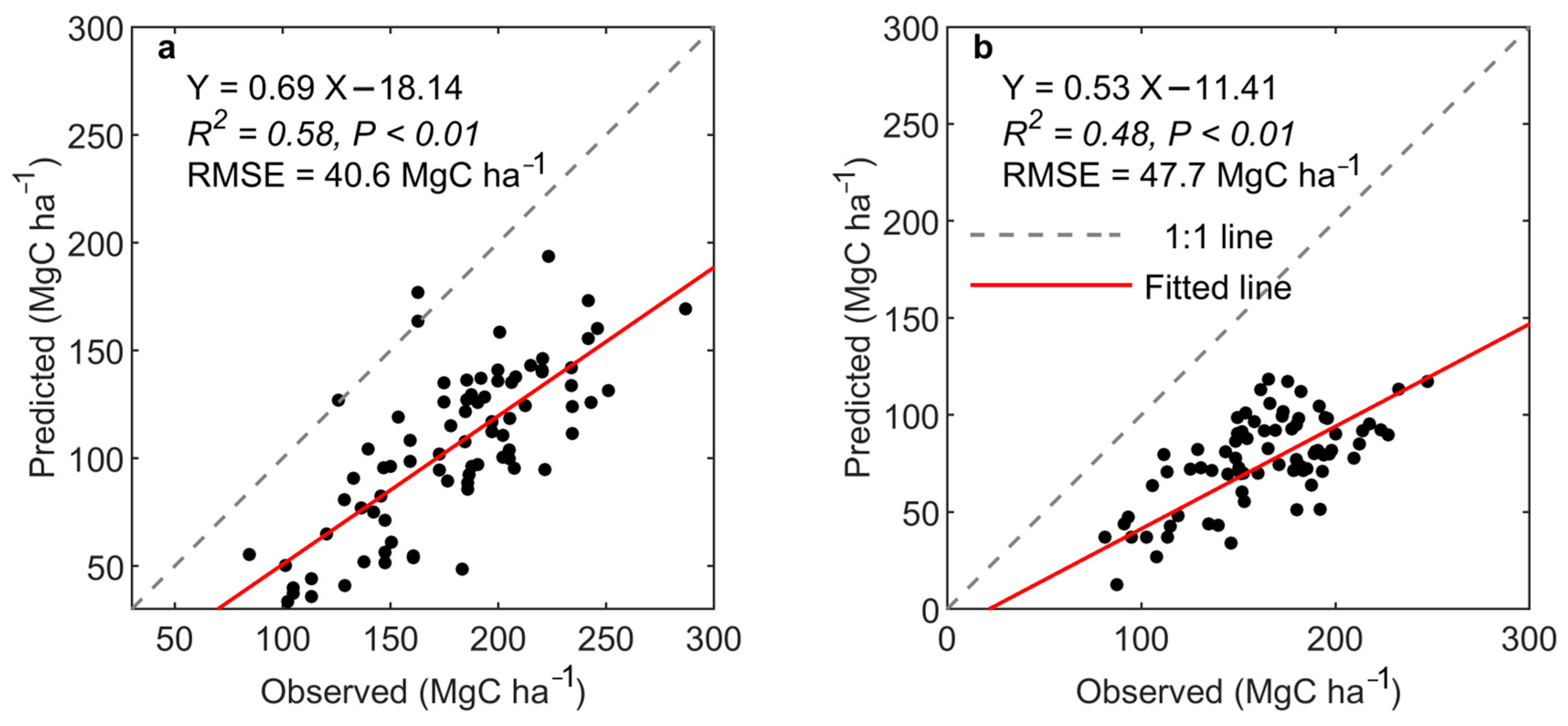
4.2.1. Comparison in Different Field Sampling Strategies

To reveal the importance of in situ observations across elevational gradients in estimating mountainous forest biomass, we compared results using elevation gradient sampling (N = 67), and with traditional random sampling from the literature review (N = 98). The comparison revealed that elevational gradient sampling strategy, though small in numbers (67 vs. 98), surpassed traditional random sampling strategy in R2 by 15.1% (Table 2) in terms of estimating mountain forest biomass. We further assessed the impact of elevational interval settings of in situ measurements on the results, considering intervals of 100 m (N = 67), 200 m (N = 32), 300 m (N = 19), and 500 m (N = 12). Here, one measurement was randomly selected at each interval, and the Monte Carlo method [53] was used to augment the sample size, ensuring a consistent sample size after sampling. The results showed that as the elevational interval increased, the accuracy of the results decreased rapidly, with R2 dropping from 0.63 to 0.51 and RMSE increasing from 22.4 to 24.8 MgC ha−1. These results highlighted the crucial role of field observation data spanning different elevational gradients, and emphasizes the need for comprehensive sampling strategies that capture the variability in forest characteristics along elevation gradients to improve the accuracy of biomass estimates in complex mountain ecosystems.

4.2.2. Comparison of Different Sources of Remote Sensing Data

Multi-source remote sensing data offer a comprehensive view of vegetation structure, with Sentinel-2 and Landsat providing information on leaf characteristics; Sentinel-1 C band backscatter reflecting trunk and branch features, and L-VOD indicating vegetation water content. We first revealed a relationship between each remote sensing data and forest biomass at the field measurement scale. Scatter plots (Figure 4) indicated that the Sentinel-1 VV and VH bands (Figure 4a,b) outperform L-VOD (Figure 4c) and optical data from Sentinel-2 (Figure 4d–g) and Landsat (Figure 4h,i) in predicting field-measured forest biomass. However, Sentinel-1 data still saturated at high forest biomass above 150 MgC ha−1, potentially underestimating high-biomass forests. Here, it should be emphasized that the weaker performance of L-VOD for biomass may be due to the loss of information and blurring caused by its lower resolution data. Furthermore, we conducted a comparative analysis using different sources of remote sensing data. Our analysis revealed that relying solely on single-source remote sensing data yielded limited accuracy in estimating forest biomass (Table 3). For instance, using Sentinel-2 and Landsat data alone to capture leaf characteristics resulted in an incomplete representation of forest structure and subsequently led to suboptimal biomass estimates (R2 = 0.65, RMSE = 23.3 MgC ha−1). It was noted that using optical data alone could significantly bias mountain forest biomass, as the underestimation could reach ~50% when compared with multi-source data results (107.0 ± 11.0 MgC ha−1 vs. 162.8 ± 21.9 MgC ha−1). Similarly, employing Sentinel-1 data, which primarily reflects trunk and branch characteristics, provided only a partial insight into forest biomass dynamics (R2 = 0.57, RMSE = 28.7 MgC ha−1). In contrast, when integrating multi-source remote sensing data, including Sentinel-2, Landsat, Sentinel-1, and L-VOD, our model achieved significantly improved performance in estimating forest biomass (R2 = 0.80, RMSE = 15.8 MgC ha−1). By leveraging the complementary information from each data source, our model was able to capture a more comprehensive range of vegetation structure features, leading to enhanced accuracy in biomass estimation.

4.2.3. Comparison with Pixel-Based Method

To reveal the effectiveness of incorporating spatial context into the ResNet model for enhancing forest biomass estimation, we conducted a comparative analysis with traditional pixel-based machine learning methods. Here, training and validation samples were kept the same. The ResNet model, equipped with convolutional layers capable of capturing spatial features within the forest canopy, outperformed traditional pixel-based methods such as RF (R2 = 0.59, RMSE = 29.3 MgC ha−1) and SVM (R2 = 0.56, RMSE = 30.4 MgC ha−1). This superiority was evident in the evaluation results presented in Table 4, where ResNet exhibited higher accuracy levels, particularly during validation at the plot scale. Additionally, XGBoost outperformed other machine learning methods with an R2 value of approximately 0.66. However, its performance remains weaker than that of the ResNet model. This is primarily because XGBoost, despite algorithmic improvements [21,54], operates on individual pixels and lacks a convolutional structure, which prevents it from fully exploring spatial distributions like ResNet does. To ascertain the impact of the convolutional structure, that could consider the spatial context in ResNet, we constructed a pixel-based DNN model devoid of convolutional layers. This model relied solely on single-pixel information for forest biomass estimation and has other structures same to ResNet. Our analysis revealed a marked discrepancy in performance, with the DNN model trailing behind CNN notably (R2 = 0.68 vs. 0.81, RMSE = 24.1 vs. 15.6 MgC ha−1). This disparity highlighted the critical role played by the convolutional structure. Incorporating spatial context allowed a model like ResNet to “understand” and process such multi-dimensional data, enabling it to recognize and analyze complex patterns and relationships within the data that are essential for accurate forest biomass estimation, especially in challenging and varied landscapes like mountainous regions.

4.2.4. Comparison with Other Advanced Deep Learning Methods

To reveal the effectiveness of including residual learning and deep neural network structures in the ResNet model for enhancing forest biomass estimation, we compared results with two other advanced convolution-based deep learning methods: AlexNet and VGG. AlexNet, with its simple three-layered architecture, offered a baseline with shallow depth, while VGG presented a more intricate setup with eight layers, yet without the residual learning integral to ResNet. Our comparative analysis indicated that the shallow depth model AlexNet performed poorly, achieving a model accuracy of only 87.5% (Table 5). Although increasing the depth of the model appeared to improve the performance of VGG, it still did not match that of ResNet. VGG’s accuracy lagged by 7.5%, potentially owing to the absence of residual connections, which are vital for the efficient training of deep networks. Residual connections streamline in ResNet introduced “shortcuts” that skip layers, simplifying gradient backpropagation and preventing diminishing gradients. This approach speeded up training while maintaining data integrity, enabling deeper network structures without added complexity. In this way, ResNet could reach high accuracy with complex deep networks in forest biomass mapping.

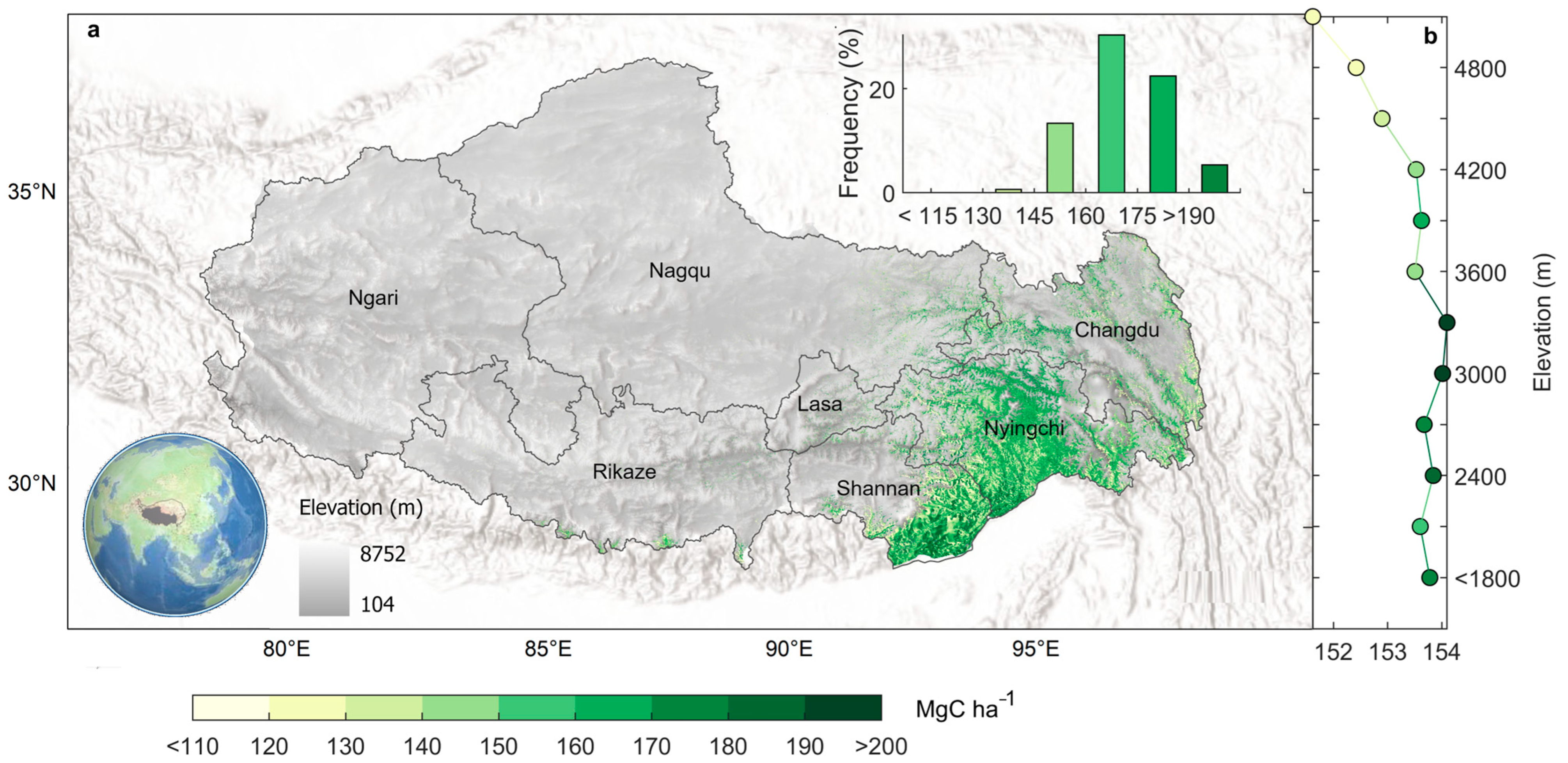
4.3. Benchmark Mapping of Mountainous Forest Biomass over Tibet

After obtaining satisfactory validation results at the plot scale, we proceeded to generate a comprehensive wall-to-wall forest biomass map for the year 2020 (Figure 5). Our analysis revealed that regional forest biomass ranges from 95.2 to 275.3 MgC ha−1, with an average of 162.8 ± 21.3 MgC ha−1. This equals a total carbon storage of approximately 2.05 PgC, constituting 40.2% of the entire forest carbon storage 5.10 PgC on the Tibetan Plateau [55]. Notably, the mountainous forests harbor high carbon density, with nearly 90% of the forest biomass exceeding 135 MgC ha−1. This is significantly higher than forests in eastern regions at similar latitudes in China (86.0 ± 10.6 MgC ha−1) [56], as well as flat regions (slopes lower than 10 degrees) in China (61.3 ± 22.4 MgC ha−1). Forest biomass reveals large spatial variation, regions with higher forest biomass are predominantly concentrated in Shannan City, situated in the southeastern part of Tibet, where the average biomass is approximately 1.24 times higher than that of the entire Tibetan region (202.4 ± 24.3 MgC ha−1). Conversely, regions such as Nagqu and Chamdo in northeastern Tibet exhibit relatively lower forest biomass, attributed to the constraints of low temperature and limited water availability. Furthermore, forest biomass exhibits significant variation with the elevation. With increasing elevation, the forest biomass accumulation began to be inhibited.

4.4. Forest Biomass Carbon Sink over Tibet

We then estimate changes in forest biomass during 2015–2020 (Figure 6). The mean forest biomass increased from 162.3 to 168.2 MgC ha−1, resulting in regional carbon storage increasing from 0.85 to 1.07 PgC. This indicates an annual forest biomass carbon sink of 3.35 ± 0.08 TgC year−1. Warming and wetting climate, along with CO2 fertilization contributed to the forest biomass carbon sink [57,58]. The size of the carbon sink varied significantly across the elevation, with lower elevation forests (below 2500 m) generally experiencing a larger carbon sink. Local forest afforestation and natural forest protection projects likely contributed to this observed increase in carbon sink size [59]. High-elevation forests (above 4000 m) constitute only 32.9% of the total forest area in Tibet, yet their carbon sink capacity accounts for 41.8% (1.40 TgC year−1) of the total carbon sink. Notably, forests near the treeline (elevation > 4500 m) also make a substantial contribution to carbon sequestration, with an annual carbon sink of 0.97 ± 0.03 TgC year−1. The warming climate would facilitate trees upslope expansion [60], which also contributes to the regional carbon sink.
We further compared our results with existing forest biomass carbon sink estimation (Table 6). Xu et al. [24] estimated global forest aboveground biomass and biomass carbon sink using a random forest method combined with ICESat/GLAS lidar data, MODIS, SRTM digital elevation model, and climate variables. We transformed aboveground biomass into total biomass, considering the root-to-shoot ratio. Liu et al. [8] provide changes in forest biomass based on VOD datasets. However, compared to our results, the previous estimation of mountainous forest biomass carbon sink (0.0068–1.19 TgC year−1) [8,24] is less than half of our results. The underestimation of forest biomass carbon sink is primarily attributed to the underestimation of mountain forest carbon stocks (0.01–0.7 PgC) in Tibet due to the lack of forest structure information and valid in situ measurement data. Specifically, the mean forest biomass over mountainous Tibet reaches only 40.0 and 102.9 MgC ha−1, which is 4 times less than our estimation. The validation results using our independent samples (N = 62) indicate that neither of these datasets effectively estimates the biomass of forests in the Tibetan region (Figure 7). This comparison shows models lacking representative field observation and spatial context can notably undervalue the biomass of mountain forests.

4.5. Limitation and Perspective

Here, we revealed significant elevational distribution of mountain forest biomass carbon stock and sink. However, the temporal mismatch between observation data (2015–2023) and our analysis period (2015–2020) could introduce uncertainties. Field observations were scarce at high elevations, especially near the treeline, and we lack repeated sampling to quantify biomass changes at the field scale. Future studies should include repeated sampling, particularly at high elevations. Furthermore, forest biomass varied greatly across sunny and shaded slopes, but we lack detailed comparative data on terrain aspect-related differences along the elevation gradient. Finer sampling could refine our understanding of microtopography’s impact on forest biomass and the carbon cycle in mountainous regions. Regarding remote sensing, we utilized optical, SAR, and VOD data for mapping forest biomass but omitted satellite LiDAR data from sources like ICESat/GLAS, ICESat-2 and GEDI. Integrating canopy height and direct vertical structure data from these sources might enhance our biomass estimates and provide better insights into the carbon cycle of mountain forests.

5. Conclusions

In summary, our study advances the benchmark mapping of forest biomass and biomass carbon sinks in mountainous regions. We introduce a deep learning-based method that integrates microwave remote sensing (C band data from Sentinel-1, and L-VOD data) with optical images (Sentinel-2A and Landsat 8). The Resnet model used in our study could automatically learn information from complex spatial features and distribution characteristics unique to mountainous forests, evidenced by comparison with the pixel-based method, advanced deep learning methods, and single-source remote sensing data. Our research also presents high-resolution (10 m) mapping of biomass and biomass carbon sink dynamics across mountainous forests during 2015–2020, thereby aiding in our understanding of how forests respond to climate change, especially in rugged mountainous regions. The magnitude of the forest carbon sink across high elevations of mountains can serve as a basis for formulating regional strategies to enhance carbon sequestration in response to climate change. However, it should be noted that our estimation still lacks observation data near the upper range limit of trees, especially near the treeline position due to the difficulty of access. The use of UAV-based or satellite-based LiDAR may be promising in those high-elevational forest carbon accounting.

Author Contributions

Conceptualization, X.W.; methodology, X.W. and G.L.; writing—original draft preparation, G.L., X.W. and J.X.; writing—review and editing, X.W., X.H., S.L., G.C. and H.H.; funding acquisition, X.W. and H.H. All authors have read and agreed to the published version of the manuscript.

Funding

This study was supported by the National Natural Science Foundation of China (42371118, 41977401) and the Science and Technology Plan Project of Tibet Autonomous Region (XZ202201ZD0005G01).

Data Availability Statement

All computer codes used in this study can be provided by the corresponding author upon reasonable request.

Acknowledgments

We thank the reviewers for their valuable comments and suggestions, and gratefully acknowledge the INRAE BORDEAUX remote sensing products for providing the SMOS-ICV2-RE06 L-VOD product (L-VOD) data.

Conflicts of Interest

The authors declare no conflicts of interest.

References

  1. Price, M.F.; Gratzer, G.; Duguma, L.A.; Kohler, T.; Maselli, D.; Romeo, R. Mountain Forests in a Changing World: Realizing Values, Adressing Challenges; FAO/SDC: Rome, Italy, 2011; pp. 1–86. [Google Scholar]
  2. Yang, Y.; Shi, Y.; Sun, W.; Chang, J.; Zhu, J.; Chen, L.; Wang, X.; Guo, Y.; Zhang, H.; Fang, J.; et al. Terrestrial carbon sinks in China and around the world and their contribution to carbon neutrality. Sci. China Life Sci. 2022, 65, 861–895. [Google Scholar] [CrossRef] [PubMed]
  3. Piao, S.; Yue, C.; Ding, J.; Guo, Z. Perspectives on the role of terrestrial ecosystems in the ‘carbon neutrality’strategy. Sci. China Earth Sci. 2022, 65, 1178–1186. [Google Scholar] [CrossRef]
  4. Pan, Y.; Birdsey, R.A.; Fang, J.; Houghton, R.; Kauppi, P.E.; Kurz, W.A.; Phillips, O.L.; Shvidenko, A.; Lewis, S.L.; Canadell, J.G.; et al. A Large and Persistent Carbon Sink in the World’s Forests. Science 2011, 333, 988–993. [Google Scholar] [CrossRef] [PubMed]
  5. Bonan, G.B. Forests and climate change: Forcings, feedbacks, and the climate benefits of forests. Science 2008, 320, 1444–1449. [Google Scholar] [CrossRef] [PubMed]
  6. Diogo, I.J.S.; dos Santos, K.; da Costa, I.R.; dos Santos, F.A.M. Effects of topography and climate on Neotropical mountain forests structure in the semiarid region. Appl. Veg. Sci. 2021, 24, e12527. [Google Scholar] [CrossRef]
  7. Greenwood, S.; Chen, J.C.; Chen, C.T.; Jump, A.S. Strong topographic sheltering effects lead to spatially complex treeline advance and increased forest density in a subtropical mountain region. Glob. Chang. Biol. 2014, 20, 3756–3766. [Google Scholar] [CrossRef] [PubMed]
  8. Liu, Y.Y.; Van Dijk, A.I.J.M.; De Jeu, R.A.M.; Canadell, J.G.; Mccabe, M.F.; Evans, J.P.; Wang, G. Recent reversal in loss of global terrestrial biomass. Nat. Clim. Chang. 2015, 5, 470–474. [Google Scholar] [CrossRef]
  9. Cutler, M.; Boyd, D.S.; Foody, G.M.; Vetrivel, A. Estimating tropical forest biomass with a combination of SAR image texture and Landsat TM data: An assessment of predictions between regions. ISPRS J. Photogramm. Remote Sens. 2012, 70, 66–77. [Google Scholar] [CrossRef]
  10. Schepaschenko, D.; Shvidenko, A.; Usoltsev, V.; Lakyda, P.; Luo, Y.; Vasylyshyn, R.; Lakyda, I.; Myklush, Y.; See, L.; McCallum, I.; et al. A dataset of forest biomass structure for Eurasia. Sci. Data 2017, 4, 170070. [Google Scholar] [CrossRef]
  11. Körner, C.; Donoghue, M.; Fabbro, T.; Häuse, C.; Nogués-Bravo, D.; Arroyo, M.T.K.; Soberon, J.; Speers, L.; Spehn, E.M.; Sun, H.; et al. Creative use of mountain biodiversity databases: The Kazbegi research agenda of GMBA-DIVERSITAS. Mt. Res. Dev. 2007, 27, 276–281. [Google Scholar] [CrossRef]
  12. Li, A.; Wang, A.; Liang, S.; Zhou, W. Eco-environmental vulnerability evaluation in mountainous region using remote sensing and GIS—A case study in the upper reaches of Minjiang River, China. Ecol. Model. 2006, 192, 175–187. [Google Scholar] [CrossRef]
  13. Xie, X.; Li, A. An adjusted two-leaf light use efficiency model for improving GPP simulations over mountainous areas. J. Geophys. Res. Atmos. 2020, 125, e2019JD031702. [Google Scholar] [CrossRef]
  14. Bian, J.; Li, A.; Lei, G.; Zhang, Z.; Nan, X. Global high-resolution mountain green cover index mapping based on Landsat images and Google Earth Engine. ISPRS J. Photogramm. Remote Sens. 2020, 162, 63–76. [Google Scholar] [CrossRef]
  15. Xie, X.; Li, A. Development of a topographic-corrected temperature and greenness model (TG) for improving GPP estimation over mountainous areas. Agric. For. Meteorol. 2020, 295, 108193. [Google Scholar] [CrossRef]
  16. Forkuor, G.; Zoungrana, J.B.B.; Dimobe, K.; Ouattara, B.; Vadrevu, K.P.; Tondoh, J.E. Above-ground biomass mapping in West African dryland forest using Sentinel-1 and 2 datasets-A case study. Remote Sens. Environ. 2020, 236, 111496. [Google Scholar] [CrossRef]
  17. Nandy, S.; Srinet, R.; Padalia, H. Mapping forest height and aboveground biomass by integrating ICESat-2, Sentinel-1 and Sentinel-2 data using Random Forest algorithm in northwest Himalayan foothills of India. Geophys. Res. Lett. 2021, 48, e2021GL093799. [Google Scholar] [CrossRef]
  18. Reiche, J.; Mullissa, A.; Slagter, B.; Gou, Y.; Tsendbazar, N.-E.; Odongo-Braun, C.; Vollrath, A.; Weisse, M.J.; Stolle, F.; Pickens, A.; et al. Forest disturbance alerts for the Congo Basin using Sentinel-1. Environ. Res. Lett. 2021, 16, 024005. [Google Scholar] [CrossRef]
  19. Zhao, P.; Lu, D.; Wang, G.; Wu, C.; Huang, Y.; Yu, S. Examining Spectral Reflectance Saturation in Landsat Imagery and Corresponding Solutions to Improve Forest Aboveground Biomass Estimation. Remote Sens. 2016, 8, 469. [Google Scholar] [CrossRef]
  20. López-Serrano, P.M.; Cárdenas Domínguez, J.L.; Corral-Rivas, J.J.; Jiménez, E.; López-Sánchez, C.A.; Vega-Nieva, D.J. Modeling of aboveground biomass with Landsat 8 OLI and machine learning in temperate forests. Forests 2019, 11, 11. [Google Scholar] [CrossRef]
  21. Li, Y.; Li, M.; Li, C.; Liu, Z. Forest aboveground biomass estimation using Landsat 8 and Sentinel-1A data with machine learning algorithms. Sci. Rep. 2020, 10, 9952. [Google Scholar] [CrossRef]
  22. Sinha, S.; Jeganathan, C.; Sharma, L.K.; Nathawat, M.S. A review of radar remote sensing for biomass estimation. Int. J. Environ. Sci. Technol. 2015, 12, 1779–1792. [Google Scholar] [CrossRef]
  23. Braun, A.; Wagner, J.; Hochschild, V. Above-ground biomass estimates based on active and passive microwave sensor imagery in low-biomass savanna ecosystems. J. Appl. Remote Sens. 2018, 12, 046027. [Google Scholar] [CrossRef]
  24. Xu, L.; Saatchi, S.S.; Yang, Y.; Yu, Y.; Pongratz, J.; Bloom, A.A.; Bowman, K.; Worden, J.; Liu, J.; Yin, Y.; et al. Changes in global terrestrial live biomass over the 21st century. Sci. Adv. 2021, 7, eabe9829. [Google Scholar] [CrossRef] [PubMed]
  25. Gleason, C.J.; Im, J. Forest biomass estimation from airborne LiDAR data using machine learning approaches. Remote Sens. Environ. 2012, 125, 80–91. [Google Scholar] [CrossRef]
  26. Mitchard, E.T.A.; Saatchi, S.S.; Woodhouse, I.H.; Nangendo, G.; Ribeiro, N.S.; Williams, M.; Ryan, C.M.; Lewis, S.L.; Feldpausch, T.R.; Meir, P. Using satellite radar backscatter to predict above-ground woody biomass: A consistent relationship across four different African landscapes. Geophys. Res. Lett. 2009, 36. [Google Scholar] [CrossRef]
  27. Rostan, F.; Riegger, S.; Pitz, W.; Torre, A.; Torres, R. The C-SAR instrument for the GMES sentinel-1 mission. In Proceedings of the 2007 IEEE International Geoscience and Remote Sensing Symposium, Barcelona, Spain, 23–28 July 2007; pp. 215–218. [Google Scholar]
  28. Sonobe, R. Combining ASNARO-2 XSAR HH and Sentinel-1 C-SAR VH/VV polarization data for improved crop mapping. Remote Sens. 2019, 11, 1920. [Google Scholar] [CrossRef]
  29. Ghosh, S.M.; Behera, M.D. Aboveground biomass estimation using multi-sensor data synergy and machine learning algorithms in a dense tropical forest. Appl. Geogr. 2018, 96, 29–40. [Google Scholar] [CrossRef]
  30. Santi, E.; Paloscia, S.; Pettinato, S.; Fontanelli, G.; Mura, M.; Zolli, C.; Maselli, F.; Chiesi, M.; Bottai, L.; Chirici, G. The potential of multifrequency SAR images for estimating forest biomass in Mediterranean areas. Remote Sens. Environ. 2017, 200, 63–73. [Google Scholar] [CrossRef]
  31. Berninger, A.; Lohberger, S.; Staengel, M.; Siegert, F. SAR-Based Estimation of Above-Ground Biomass and Its Changes in Tropical Forests of Kalimantan Using L- and C-Band. Remote Sens. 2018, 10, 831. [Google Scholar] [CrossRef]
  32. Tian, F.; Brandt, M.; Liu, Y.Y.; Verger, A.; Tagesson, T.; Diouf, A.A.; Rasmussen, K.; Mbow, C.; Wang, Y.; Fensholt, R. Remote sensing of vegetation dynamics in drylands: Evaluating vegetation optical depth (VOD) using AVHRR NDVI and in-situ green biomass data over West African Sahel. Remote Sens. Environ. 2016, 177, 265–276. [Google Scholar] [CrossRef]
  33. Wang, M.; Fan, L.; Frappart, F.; Ciais, P.; Sun, R.; Liu, Y.; Li, X.; Liu, X.; Moisy, C.; Wigneron, J.-P. An alternative AMSR2 vegetation optical depth for monitoring vegetation at large scales. Remote Sens. Environ. 2021, 263, 112556. [Google Scholar] [CrossRef]
  34. Rodríguez-Fernández, N.J.; Mialon, A.; Mermoz, S.; Bouvet, A.; Richaume, P.; Al Bitar, A.; Al-Yaari, A.; Brandt, M.; Kaminski, T.; Le Toan, T.; et al. An evaluation of SMOS L-band vegetation optical depth (L-VOD) data sets: High sensitivity of L-VOD to above-ground biomass in Africa. Biogeosciences 2018, 15, 4627–4645. [Google Scholar] [CrossRef]
  35. Fan, L.; Wigneron, J.-P.; Ciais, P.; Chave, J.; Brandt, M.; Fensholt, R.; Saatchi, S.S.; Bastos, A.; Al-Yaari, A.; Hufkens, K.; et al. Satellite-observed pantropical carbon dynamics. Nat. Plants 2019, 5, 944–951. [Google Scholar] [CrossRef] [PubMed]
  36. Wigneron, J.P.; Fan, L.; Ciais, P.; Bastos, A.; Brandt, M.; Chave, J.; Saatchi, S.; Baccini, A.; Fensholt, R. Tropical forests did not recover from the strong 2015–2016 El Niño event. Sci. Adv. 2020, 6, eaay4603. [Google Scholar] [CrossRef] [PubMed]
  37. Dou, Y.; Tian, F.; Wigneron, J.-P.; Tagesson, T.; Du, J.; Brandt, M.; Liu, Y.; Zou, L.; Kimball, J.S.; Fensholt, R. Reliability of using vegetation optical depth for estimating decadal and interannual carbon dynamics. Remote Sens. Environ. 2023, 285, 113390. [Google Scholar] [CrossRef]
  38. Konings, A.G.; Saatchi, S.S.; Frankenberg, C.; Keller, M.; Leshyk, V.; Anderegg, W.R.L.; Humphrey, V.; Matheny, A.M.; Trugman, A.; Sack, L.; et al. Detecting forest response to droughts with global observations of vegetation water content. Glob. Chang. Biol. 2021, 27, 6005–6024. [Google Scholar] [CrossRef] [PubMed]
  39. Holtzman, N.M.; Anderegg, L.D.L.; Kraatz, S.; Mavrovic, A.; Sonnentag, O.; Pappas, C.; Cosh, M.H.; Langlois, A.; Lakhankar, T.; Tesser, D.; et al. L-band vegetation optical depth as an indicator of plant water potential in a temperate deciduous forest stand. Biogeosciences 2021, 18, 739–753. [Google Scholar] [CrossRef]
  40. Luo, K.; Wei, Y.; Du, J.; Liu, L.; Luo, X.; Shi, Y.; Pei, X.; Lei, N.; Song, C.; Li, J.; et al. Machine learning-based estimates of aboveground biomass of subalpine forests using Landsat 8 OLI and Sentinel-2B images in the Jiuzhaigou National Nature Reserve, Eastern Tibet Plateau. J. For. Res. 2022, 33, 1329–1340. [Google Scholar] [CrossRef]
  41. Li, T.; Zou, Y.; Liu, Y.; Luo, P.; Xiong, Q.; Lu, H.; Lai, C.; Axmacher, J.C. Mountain forest biomass dynamics and its drivers in southwestern China between 1979 and 2017. Ecol. Indic. 2022, 142, 109289. [Google Scholar] [CrossRef]
  42. Huang, J.; Wang, X.; Zhao, Y.; Xin, C.; Xiang, H. Large Earthquake Magnitude Prediction In Taiwan Based On Deep Learning Neural Network. Neural Netw. World 2018, 28, 149–160. [Google Scholar] [CrossRef]
  43. Liang, P.; Wang, X.; Sun, H.; Fan, Y.; Wu, Y.; Lin, X.; Chang, J. Forest type and height are important in shaping the altitudinal change of radial growth response to climate change. Sci. Rep. 2019, 9, 1336. [Google Scholar] [CrossRef] [PubMed]
  44. Zhong, L.; Hu, L.; Zhou, H. Deep learning based multi-temporal crop classification. Remote Sens. Environ. 2019, 221, 430–443. [Google Scholar] [CrossRef]
  45. Kattenborn, T.; Leitloff, J.; Schiefer, F.; Hinz, S. Review on Convolutional Neural Networks (CNN) in vegetation remote sensing. ISPRS J. Photogramm. Remote Sens. 2021, 173, 24–49. [Google Scholar] [CrossRef]
  46. Wang, G.; Ran, F.; Chang, R.; Yang, Y.; Luo, J.; Fan, J. Variations in the live biomass and carbon pools of Abies georgei along an elevation gradient on the Tibetan Plateau, China. For. Ecol. Manag. 2014, 329, 255–263. [Google Scholar] [CrossRef]
  47. Sun, X.; Wang, G.; Huang, M.; Chang, R.; Ran, F. Forest biomass carbon stocks and variation in Tibet’s carbon-dense forests from 2001 to 2050. Sci. Rep. 2016, 6, 34687. [Google Scholar] [CrossRef]
  48. Zhu, H. The Tropical Forests of Southern China and Conservation of Biodiversity. Bot. Rev. 2017, 83, 87–105. [Google Scholar] [CrossRef]
  49. Li, W.; Ciais, P.; Guenet, B.; Peng, S.; Chang, J.; Chaplot, V.; Khudyaev, S.; Peregon, A.; Piao, S.; Wang, Y.; et al. Temporal response of soil organic carbon after grassland-related land-use change. Glob. Chang. Biol. 2018, 24, 4731–4746. [Google Scholar] [CrossRef]
  50. Gorelick, N.; Hancher, M.; Dixon, M.; Ilyushchenko, S.; Thau, D.; Moore, R. Google Earth Engine: Planetary-scale geospatial analysis for everyone. Remote Sens. Environ. 2017, 202, 18–27. [Google Scholar] [CrossRef]
  51. Simonyan, K.; Zisserman, A. Very deep convolutional networks for large-scale image recognition. arXiv 2014, arXiv:1409.1556. [Google Scholar]
  52. Abadi, M.; Barham, P.; Chen, J.; Chen, Z.; Davis, A.; Dean, J.; Devin, M.; Ghemawat, S.; Irving, G.; Isard, M.; et al. TensorFlow: A system for large-scale machine learning. In Proceedings of the 12th USENIX Symposium on Operating Systems Design and Implementation (OSDI 16), Savannah, GA, USA, 2–4 November 2016; Volume 16, pp. 265–283. [Google Scholar]
  53. Del Moral, P.; Doucet, A.; Jasra, A. On adaptive resampling strategies for sequential Monte Carlo methods. Bernoulli 2012, 18, 252–278. [Google Scholar] [CrossRef]
  54. Bartold, M.; Kluczek, M. A Machine Learning Approach for Mapping Chlorophyll Fluorescence at Inland Wetlands. Remote Sens. 2023, 15, 2392. [Google Scholar] [CrossRef]
  55. Wang, T.; Wang, X.; Liu, D.; Lv, G.; Ren, S.; Ding, J.; Chen, B.; Qu, J.; Wang, Y.; Piao, S. The current and future of terrestrial carbon balance over the Tibetan Plateau. Sci. China Earth Sci. 2023, 66, 1493–1503. [Google Scholar] [CrossRef]
  56. Spawn, S.A.; Sullivan, C.C.; Lark, T.J.; Gibbs, H.K. Harmonized global maps of above and belowground biomass carbon density in the year 2010. Sci. Data 2020, 7, 112. [Google Scholar] [CrossRef] [PubMed]
  57. Ruehr, S.; Keenan, T.F.; Williams, C.; Zhou, Y.; Lu, X.; Bastos, A.; Canadell, J.G.; Prentice, I.C.; Sitch, S.; Terrer, C. Evidence and attribution of the enhanced land carbon sink. Nat. Rev. Earth Environ. 2023, 4, 518–534. [Google Scholar] [CrossRef]
  58. Piao, S.; Zhang, Y.; Zhu, Z.; Lian, X.; Huang, K.; He, M.; Zhao, C.; Liu, D. Socioeconomic and Environmental Changes in Global Drylands. In Dryland Social-Ecological Systems in Changing Environments; Springer: Singapore, 2014; pp. 161–201. [Google Scholar]
  59. Wang, W.; Feng, C.; Liu, F.; Li, J. Biodiversity conservation in China: A review of recent studies and practices. Environ. Sci. Ecotechnol. 2020, 2, 100025. [Google Scholar] [CrossRef]
  60. Wang, X.; Wang, T.; Xu, J.; Shen, Z.; Yang, Y.; Chen, A.; Wang, S.; Liang, E.; Piao, S. Enhanced habitat loss of the Himalayan endemic flora driven by warming-forced upslope tree expansion. Nat. Ecol. Evol. 2022, 6, 890–899. [Google Scholar] [CrossRef]
Figure 1. Distribution of forests and in situ measurements over Tibet.
Remotesensing 16 01481 g001
Figure 2. Schematic flow of the mountain forest biomass and biomass carbon sink mapping proposed in this study.
Remotesensing 16 01481 g002
Figure 3. Relationship between the independent in situ measurement and the predicted forest biomass. The solid blue line and the dashed black line represent the regression line and 1:1 line, respectively. Here, independent samples (N = 62) were only used for verification. R2 represents the coefficient of determination, and RMSE is the root mean squared error.
Remotesensing 16 01481 g003
Figure 4. Relationship between the forest biomass and the multi-source remote sensing data at field measurement scale. The subplots reveal data using multi-source remote sensing data, including (a) VV, (b) VH bands from Sentinel-1, (c) Vegetation Optical Depth (VOD), (dg) reflectance data from Sentinel-2, and (hl) Landsat 8. All remote sensing-based data have been normalized.
Remotesensing 16 01481 g004
Figure 5. Spatial pattern of mountain forest biomass over Tibet in 2020. (a) Distribution of forest biomass estimated by the newly proposed deep learning method, that integrates CNN with Sentinel-1 and Landsat data. The inset displays the frequency of forest biomass. (b) Mean elevational value of forest biomass over Tibet.
Remotesensing 16 01481 g005
Figure 6. Spatial pattern of the forest biomass carbon sink between 2015 and 2020. (a) Distribution of forest biomass carbon sink. The inset displays the frequency of forest biomass carbon sink. (b) Mean elevational value of forest biomass carbon sink over Tibet. The red region indicates a decrease in biomass and the green region is an increase.
Remotesensing 16 01481 g006
Figure 7. Validation of existing forest biomass maps in mountainous areas of Tibet based on measured samples. (a,b) are the estimated results of Liu et al. [8] and Xu et al. [24], respectively.
Remotesensing 16 01481 g007
Table 1. Details of the multi-source remote sensing imagery used in this study.
Multi-Source Remote Sensing DatasetBandDescriptionSpatial Resolution
Sentinel 1VVVertical transmit–Vertical receive10 m
VHVertical transmit–Horizontal receive
VOD SMOS-ICV2-RE06L-VODVOD0.25°
Sentinel-2ABand 3Green10 m
Band 4Red
Band 8Near-infrared
Band 11Shortwave infrared
Band 12Shortwave infrared
Landsat 8 OLIBand 3Green30 m
Band 4Red
Band 5Near-infrared
Band 6Shortwave infrared
Band 7Shortwave infrared
Table 2. Estimations using different field sampling strategies.
R2RMSE (MgC ha−1)
Elevation gradient sampling
(Total, N = 67)
0.6322.4
Traditional random sampling
(N = 98)
0.5324.6
Elevation gradient sampling
(interval = 200 m, N = 32)
0.5923.9
Elevation gradient sampling
(interval = 300 m, N = 19)
0.5624.7
Elevation gradient sampling
(interval = 500 m, N = 12)
0.5124.8
Table 3. Comparison in forest biomass accuracy using different sources of remote sensing data.
FeaturesR2RMSE (MgC ha−1)
Sentinel-2A + Landsat OLI0.6523.3
Sentinel-10.5728.7
Sentinel-2A + Landsat OLI + Sentinel-10.7818.1
Sentinel-2A + Landsat OLI + Sentinel-1 + VOD0.8015.8
Table 4. Comparison with the pixel-based method for forest biomass estimation.
AlgorithmR2RMSE (MgC ha−1)
ResNet0.8015.8
DNN0.6824.1
XGBoost0.6623.3
RF0.5929.3
SVM0.5630.4
Table 5. Comparison in forest biomass accuracy using different CNN models.
AlgorithmR2RMSE (MgC ha−1)
ResNet0.8015.8
VGG0.7418.2
AlexNet0.7021.1
Table 6. Comparison in existing mountain forest biomass carbon sink estimation in Tibet.
Biomass
(MgC ha−1)
Carbon Stocks
(PgC)
Carbon Sink
(TgC year−1)
MethodData
This study162.65.103.35ResNetSentinel-2A
Landsat OLI
Sentinel-1
VOD
Liu et al. [8]40.00.010.0068The empirical relationship of convert VOD to aboveground biomass carbonVOD
Xu et al. [24]102.90.71.19Random forestGLAS
MODIS
QuikSCAT
WorldClim
SRTM
Disclaimer/Publisher’s Note: The statements, opinions and data contained in all publications are solely those of the individual author(s) and contributor(s) and not of MDPI and/or the editor(s). MDPI and/or the editor(s) disclaim responsibility for any injury to people or property resulting from any ideas, methods, instructions or products referred to in the content.

