
Effects of Ice-Microstructure-Based Inherent Optical Properties Parameterization in the CICE Model
1
State Key Laboratory of Numerical Modeling for Atmospheric Sciences and Geophysical Fluid Dynamics (LASG), Institute of Atmospheric Physics, Chinese Academy of Sciences, Beijing 100029, China
2
University of Chinese Academy of Sciences, Beijing 100045, China
3
School of Atmospheric Sciences, Sun Yat-sen University, and Southern Marine Science and Engineering Guangdong Laboratory (Zhuhai), Zhuhai 519082, China
*
Author to whom correspondence should be addressed.
Remote Sens. 2024, 16(9), 1494; https://doi.org/10.3390/rs16091494
Submission received: 5 February 2024
/
Revised: 15 April 2024
/
Accepted: 15 April 2024
/
Published: 24 April 2024
(This article belongs to the Special Issue Remote Sensing of Polar Sea Ice)
Abstract
:The constant inherent optical properties (IOPs) for sea ice currently applied in sea ice models do not realistically represent the dividing of shortwave radiative fluxes in sea ice and the ocean below it. Here we implement a parameterization of variable IOPs based on ice microstructures in the Los Alamos sea ice model, version 6.0 (CICE6) and investigate its effects on the simulation of the dividing of shortwave radiation and sea ice in the Arctic. Our sensitivity experiments indicate that variable IOP parameterization results in strong seasonal variation for the IOP parameters, typically reaching the seasonal maximum in the boreal summer. With such large differences, variable IOP parameterization leads to increased absorbed solar radiation at the surface and in the interior of Arctic sea ice relative to constant IOPs, up to ~3 W/m2, but decreased solar radiation penetrating into the ocean, up to ~5–6 W/m2. The changes in the dividing of shortwave fluxes in sea ice and the ocean below it induced by the variable IOPs have significant influence on Arctic sea ice thickness by modulating surface and bottom melting and frazil ice formation (increasing surface melting by ~16% and reducing bottom melting by ~11% in summer).
1. Introduction
The reflection, absorption, and penetration of shortwave radiation in sea ice and the ocean below it play a critical role in the energy and mass balance of Arctic sea ice [1,2,3,4]. Shortwave radiation reflected and absorbed by the ice determines surface albedo temperature feedback, which is an important factor for amplified Arctic warming [5,6,7]. It also results in surface melting, i.e., the formation of melt ponds substantially decreases surface reflection, which is a sensitive predictor of the seasonal minimum of Arctic sea ice [8,9,10]. Shortwave radiation absorbed by the ice interior results in internal melting, forming large holes within the ice, making the ice rotten, and allowing salt water intrusion [11]. The transmission of shortwave radiation through the ice can warm the ocean below the ice, resulting in bottom ice melting [8,12], modulating ice-ocean heat and salt fluxes. The shortwave radiation transmitted through the ice also enhances primary production, influencing the ecosystem in the ice-covered Arctic Ocean [13,14,15]. Thus, it is important to accurately simulate the partitioning of shortwave fluxes in sea ice and the ocean below it, and understand its influence on Arctic sea ice simulation.
Modeling correct shortwave fluxes in sea ice and the ocean below it is important for atmosphere–sea ice–ocean interactions in sea ice models and coupled climate models, leading to realistic representation of heat exchange. Previous studies have showed that shortwave fluxes in sea ice and the ocean below it are strongly modulated by the inherent optical properties (IOPs) of sea ice, which include the parameters of scattering, absorption, and asymmetry [16]. These IOP parameters are controlled by sea ice microstructures. They include air bubbles, brine droplets, and fine particulates, as well as their size, vertical distribution, and volume [17,18,19]. The brightness temperature measured by passive microwave sensors from emitted radiation by sea ice can be influenced by the brine volume of sea ice. Also, the backscattering of sea ice is influenced by the presence of gas bubbles in the sea ice [20,21,22]. Thus, the ice microstructure based IOPs is important for simulating and predicting various radiative processes that influence sea ice variation and should be taken into account in sea ice models.
As a key physical process in sea ice models, the parameterization of shortwave radiation transfer in sea ice has been improved from a relatively simple scheme in the Community Climate System Model, version 3 (CCSM3) [23] to a multiple scattering radiative transfer model, Delta-Eddington [24]. The Delta-Eddington parameterization prescribes inherent optical properties for snow-covered ice, bare ice, and melt ponds to calculate apparent optical properties, including refection, absorption, and penetration. However, the ice IOPs in the Delta-Eddington parameterization are treated as constants according to previous field observation as well as a structural-optical model [18,24,25]. Constant IOPs cannot reflect physics to be applicable to all situations, thus it is important to include a better IOP treatment to reproduce the physically realistic IOPs for the calculation of apparent optical properties.
An IOP parameterization of sea ice was developed by Grenfell, which provides a physically-based way to calculate IOPs based on refractive index, wavelength, size, and distribution of inclusions [26]. Compared to the constant IOPs, this IOP parameterization can generate spatially and temporally varying IOPs, making it applicable to different sea ice types and conditions. By identifying and quantifying key IOP parameters, a more concise representation of optical properties for sea ice can be achieved.
The objective of this study is to implement a variable IOP parameterization in a stand-alone sea ice model, and to examine the sensitivity of the modeled shortwave fluxes in Arctic sea ice and the ocean below it to the variable IOP parameterization and constant IOPs as well as their impacts on Arctic sea ice simulations.
2. Method, Data, and Sea Ice Model
2.1. IOPs Parameterization
Grenfell (1991) proposed a parameterization to compute the parameters of the scattering, absorption, and asymmetry of sea ice [26]. An analytical solution of these coefficients is derived based on the refractive index, wavelength, size, and distribution of ice inclusions. In this IOP parameterization, sea ice is considered to be a mixture of pure ice, air bubbles, brine droplets, and fine particulate, which have different effects on incoming solar radiation. Recently, the influence of such parameterization on the optical properties of summer sea ice has been examined using a Delta-Eddington multiple scattering model [19]. They assumed that pure ice only absorbs shortwave, that air bubbles only scatter shortwave, and that brine droplets and fine particulate have both scatter and absorb effects. In this study, the scattering coefficient (), absorption coefficient (), and asymmetry parameter () of sea ice are calculated as follows [26], where , , , refer to brine droplet, air bubbles, particular matter, and pure ice, respectively.
is the absorption coefficient for pure ice without bubbles, which is computed by Equation (6). is the imaginary part of the ice refraction index, which is obtained from Warren et al. [27]. is the wavelength. is the pure ice volume, is the length for each brine droplet, is the radius for each inclusion, and and are the efficiency of scattering and absorption that are computed by Mie theory, respectively [19]. For the asymmetry coefficients, is set as 0.86 and is set as 0.99 according to Light et al. [18], and is obtained using Mie theory. is the function of size distribution. Given the volume of bubbles and brine droplets , the solution of and can be derived using Equations (7) and (8); the detailed derivation can be found in Grenfell et al. and Light et al. [17,28].
where is the aspect ratio of the brine droplets.
is computed from the concentration () and radius () of PM. Here we use the same values in Yu et al. [19] except , . The gas volume fraction is set to be 3% based on the average from the field observations [29]. The brine volume fraction is calculated as follows.
where is bulk ice salinity and is brine salinity calculated in the sea ice model introduced in Section 2.3.
The coefficients of scattering and absorption computed above are then converted into extinction coefficient () and the single scattering albedo () used in sea ice models.
2.2. Atmospheric and Oceanic Forcing Data
The Japanese global atmospheric reanalysis (JRA-55) is used as the atmospheric forcings for Arctic sea ice simulation, which was developed by the Japan Meteorological Agency using an improved data assimilation system and a newly prepared dataset of past observations [30]. Every 6 h, JRA55 data are used to force a stand-alone sea ice model (see Section 2.3 for details). The atmospheric variables utilized include downward surface shortwave and longwave, 10-m U and V winds, near-surface air temperature, density and specific humidity, precipitation, and snowfall rates.
The Ocean ReAnalysis System 5 (ORAS5) developed by the European Centre for Medium-Range Weather Forecasts (ECMWF) is used as the ocean forcings for Arctic sea ice simulation, which is produced from an eddy-permitting ensemble reanalysis system for ocean and sea ice [31]. The monthly-mean ORAS5 data are used to force the sea ice model. The oceanic variables utilized include temperature and salinity at sea surface, and the depth of the mixed layer.
2.3. Sea Ice Model
To investigate the effects of the above variable IOP parameterization on simulated shortwave radiation and sea ice in the Arctic, we incorporate the parameterization into the Los Alamos sea ice model, version 6.0 [32]. CICE6 is a stand-alone model to simulate dynamics and thermodynamics of sea ice. It computes sea ice growth, melting, and movement of sea ice to describe the spatial and temporal change in ice thickness distribution. Its dynamic component consists of elastic-viscous-plastic (EVP) and elastic-anisotropic-plastic (EAP) rheologies. They compute the velocity field of the ice pack. The EVP scheme is employed here. Its thermodynamic component computes variations in the ice and snow due to a variety of thermodynamic processes, and the vertical temperature profile influenced by various heat fluxes associated with radiative, turbulent, and conductive processes.
In CICE6, a Delta-Eddington shortwave multiple scattering parameterization is used to simulate interactions between shortwave radiation and snow and sea ice. Inherent optical properties for sea ice in Delta-Eddington are prescribed as constants according to previous in situ measurements [24,25]. Table 1 shows the values of these inherent optical properties for the ice in two bands, a visible band (200–700 nm) and a near-infrared band (700–1190 nm and 1190–5000 nm). These inherent optical properties are then used in the Delta-Eddington radiative transfer model to compute absorption in sea ice and transmission to the ocean below the ice.
Here the model is run on the dipolar grid. The horizontal resolution is ∼1°(latitude) × 1° (longitude). Five ice thickness categories, one layer of snow, and seven layers of sea ice are used. In this study, the model is executed for 15 years with the repeated boundary forcings for the year of 2012. The simulation averaged for the last five years is discussed in Section 3.
3. Results
To examine the impacts of the variable IOP parameterization, we implement the parameterization as described in Section 2.1 in CICE6 to compute inherent optical properties of sea ice to replace the constant IOPs in Table 1. Here we use CICE-IOP to denote the simulation adopting the variable IOP parameterization and CICE-constant to denote the default CICE simulation with constant IOPs. Grids with simulated sea ice above 15% (the typical value used to define the sea ice edge) are considered to generate all plots.
3.1. Impacts on Inherent Optical Properties
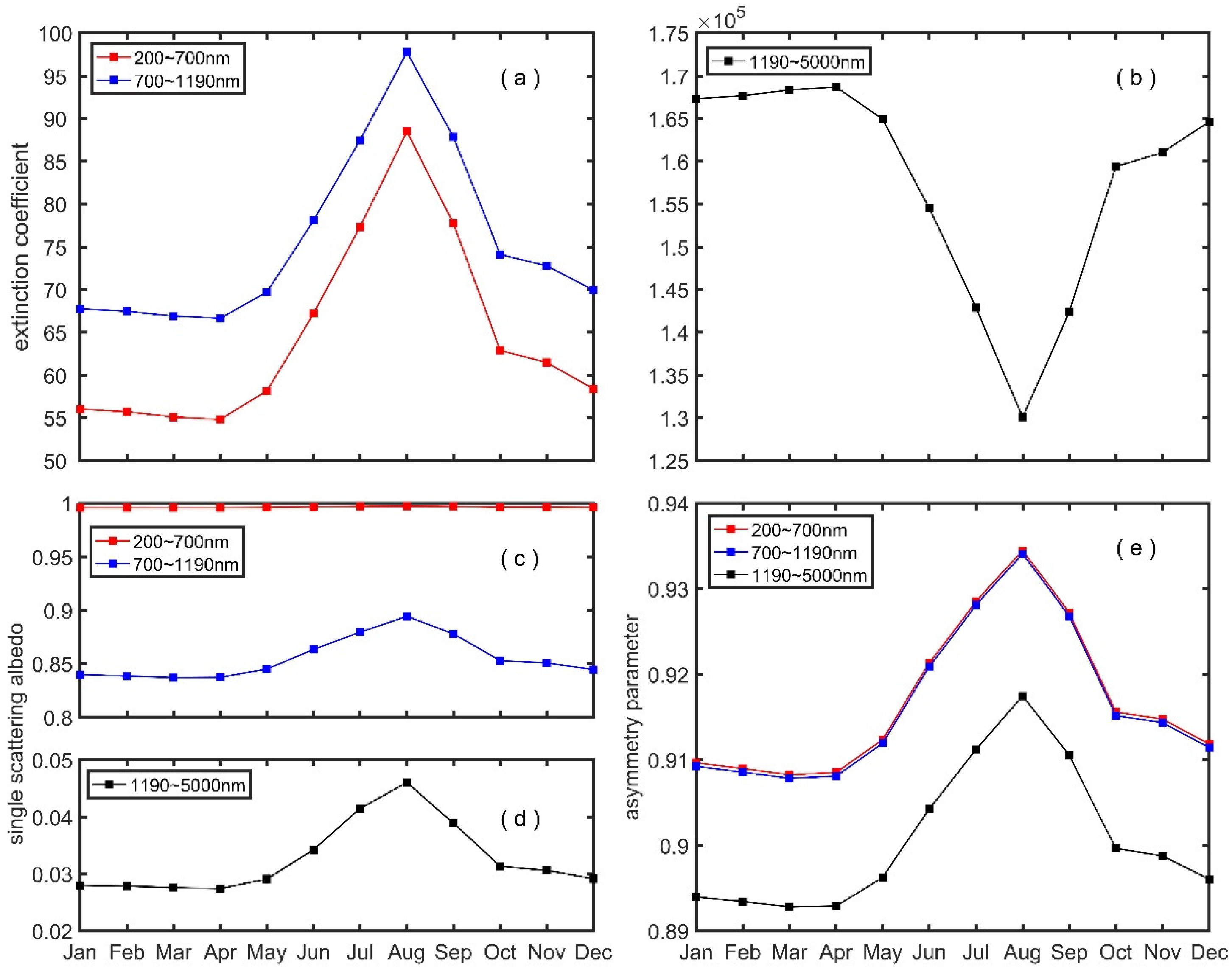
Figure 1 shows the seasonal evolution of the extinction coefficient, single scattering albedo, and asymmetry parameter averaged over the Arctic simulated by the variable IOP parameterization. The extinction coefficients in both visible and near-infrared bands (700–1190 nm) show a large seasonal variation. The visible and near-infrared (700–1190 nm) has a maximum value in August, whereas the near-infrared (1190–5000 nm) has a minimum value in August. The magnitude of the latter is five-order larger than the former due to the fact that (the imaginary part of the complex index of refraction of ice) ranges from to in band 1190–5000 nm. The extremely large means the magnitude of the absorption coefficient of ice can reach , leading to an extremely large value of extinction coefficient in band 1190–5000 nm. The single scattering albedo in the visible band is close to 1 which is similar to the CICE default constant, but in the near-infrared band, the single scattering albedo is larger than the CICE default constant, and also shows seasonal variation with a peak in summer. The asymmetry parameter simulated by the parameterization is relatively smaller than the CICE default constant, reaching a seasonal maximum in August. In our study, sea ice is considered as a mixture of pure ice, air bubbles, brine droplets, and fine particulate. Among them, brine volume fraction is calculated as the ratio of brine salinity simulated in the CICE model and bulk ice salinity, while the other inclusions are prescribed based on the field observations of Ehn et al. and Light et al. [29,33]. Thus, the simulated brine volume fraction plays a key role in determining the aforementioned seasonal variation in the IOP parameters.
3.2. Impacts on Shortwave Fluxes
Varying ice IOPs as discussed above can influence shortwave radiative fluxes absorbed by and transmitted through Arctic sea ice. Figure 2a,b shows the seasonal evolution of the simulated absorbed shortwave fluxes at the ice surface and interior averaged over the Arctic for the CICE-IOP and CICE-constant experiments. The variable IOP parameterization results in increased shortwave radiation absorbed at both the ice surface and interior compared to the CICE-constant in summer. As shown in Figure 2c, this leads to significantly decreased penetration of shortwave radiation through the ice into the ocean during the melting season relative to the CICE-constant.
The Delta-Eddington solar radiation treatment allows three types of the ice surface: snow-covered ice, bare ice, and melt ponds. Thus, we further calculate the absorbed surface radiation for the three different surfaces. As shown in Figure 3, the absorbed shortwave fluxes by the ponded ice simulated with the variable IOP parameterization is larger than the CICE-constant during the melting season, whereas the snow-covered ice and bare ice show minor change relative to ICE-constant. Figure 4 shows the variation in the melt pond fraction. Compared to the CICE-constant, CICE-IOP generates larger pond fraction, which explains the abovementioned increased absorbed solar radiation.
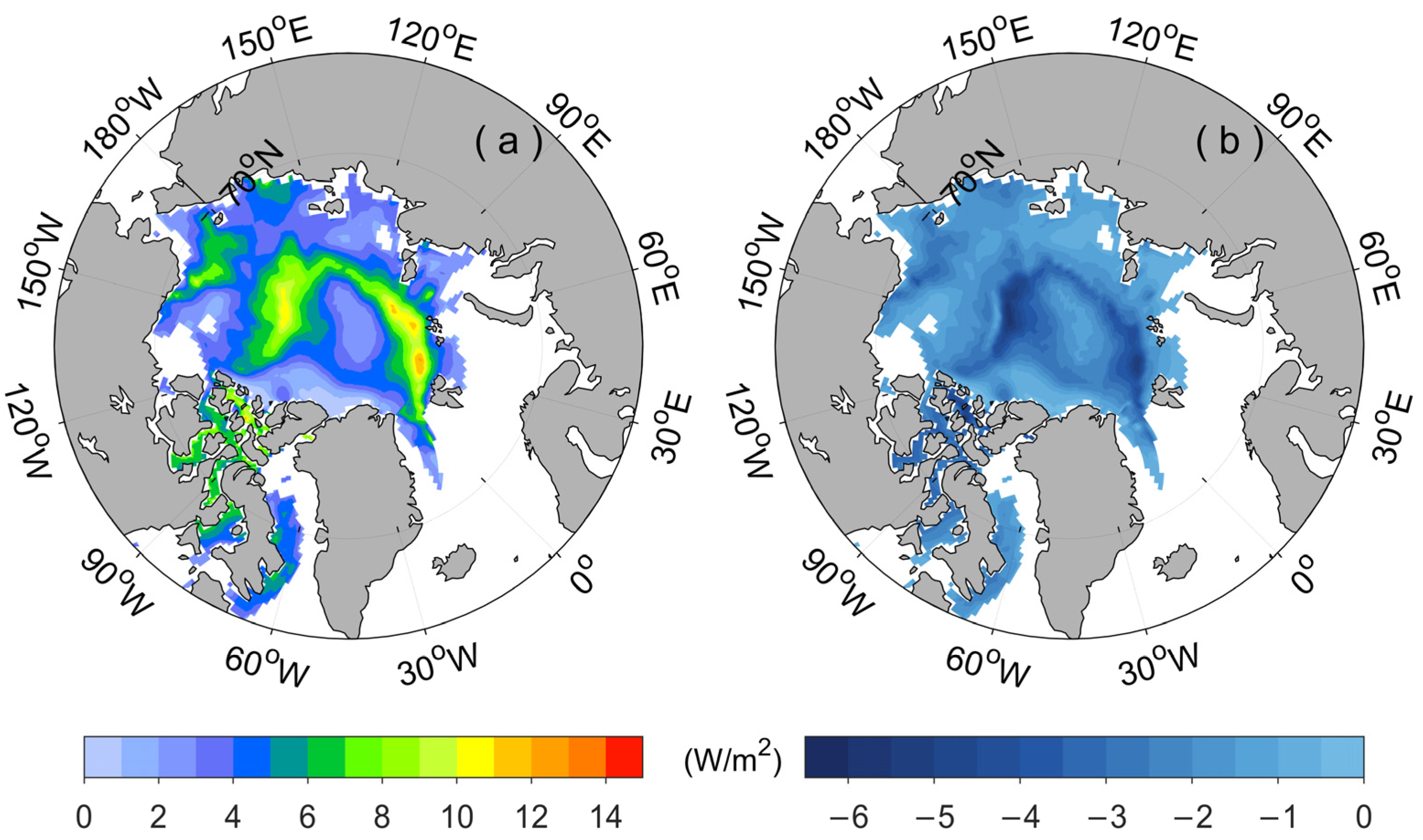
Figure 5 shows spatial distribution of absorbed shortwave fluxes at the ice surface simulated by the CICE-constant and the difference between the CICE-IOP and the CICE-constant in summer. As simulated by CICE-constant, in summer, the largest surface absorption occurs in the southern Beaufort Sea, Chukchi Sea, eastern Siberian Sea, and Canadian Arctic, which decreases towards the central Arctic and the Atlantic sector (Figure 5a). The variable IOP parameterization enhances the basin-wide absorption of shortwave fluxes at the ice surface with the largest increase ~3–4 W/m2 (Figure 5b). As shown in Figure 6a, the spatial distribution of the absorbed shortwave fluxes in the ice interior produced by the CICE-constant is generally similar to that of Figure 5a. Varying IOPs also increases the interior absorption of solar radiation in much of the Arctic, with the largest increase in the central Arctic (~2–3 W/m2, Figure 6b). Figure 7a is spatial distribution of shortwave fluxes through the ice into the ocean. The CICE-constant shows a band of large penetration of solar radiation in the Arctic. Varying IOPs result in the basin-wide decrease in shortwave fluxes available to the ocean below the ice, up to ~5–6 W/m2 (Figure 7b).
3.3. Impacts on Sea Ice Simulation
Next, the impacts of changing shortwave fluxes as discussed above on the simulation of sea ice thermodynamic processes in the Arctic are examined. We focus on each individual thermodynamic process associated with sea ice growth and melt, including basal ice growth, the formation of frazil ice, conversion from snow to ice, surface ice melt, basal ice melt, and lateral ice melt [34,35]. Figure 8a shows the seasonal variation in each term for the ice mass budget averaged for the Arctic simulated by the CICE-constant. It shows a net gain (loss) from October to April (from May to September). Among them, basal growth is the dominant contributor to the ice mass gain relative to the formation of frazil ice, conversion from snow to ice. Basal and top melt are two dominant factors for the ice mass loss. The former process occurs in spring and summer, while the latter process mainly occurs in summer.
Figure 8b shows the difference in each mass budget term between the CICE-IOP and the CICE-constant. Compared to the CICE-constant, the variable IOP parameterization increases surface melting (~16% averaged for summer, Figure 9) and reduces bottom melting (~11% averaged for summer, Figure 9) during the melting season. This is consistent with the aforementioned changes in shortwave radiative fluxes. Varying IOPs also leads to an increase in bottom melting in early fall. In addition, the CICE-IOP results in an increase in frazil ice from May to September (66% averaged for summer, Figure 9). Other processes show minimal changes, though the bottom growth shows a small increase.
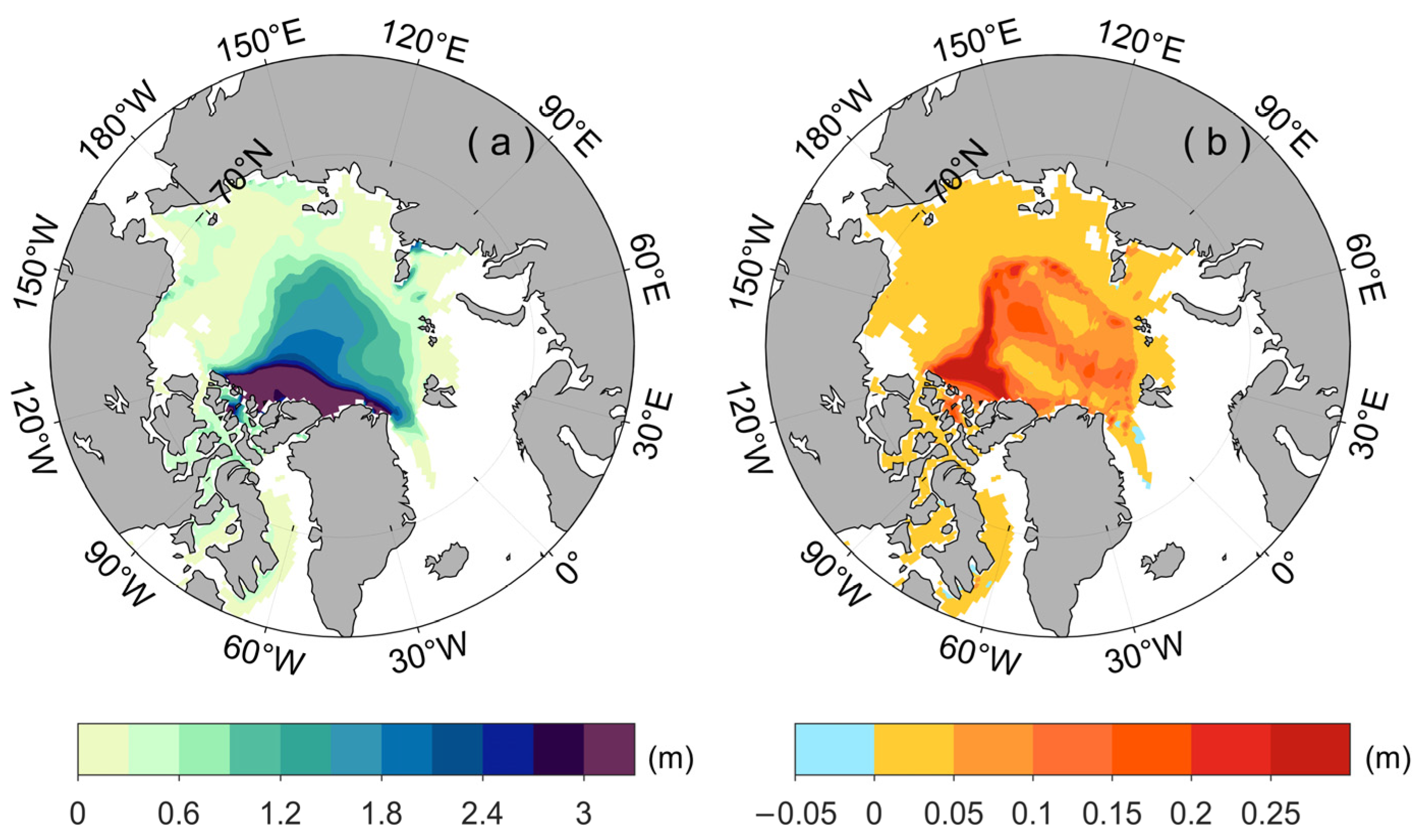
Figure 10 compares the seasonal variation in the extent of Arctic sea ice extent for the two numerical experiments. It appears that the difference between CICE-IOP and CICE-constant is minimal (Figure 10), though CICE-IOP has relatively more ice cover in August and September. By contrast, the simulated seasonal variation in the mean Arctic sea ice thickness shows an obvious difference between the two experiments; CICE-IOP leads to thicker ice than that of the CICE-constant for all months, especially from August to October (Figure 11). Spatially, the variable IOP parameterization results in an Arctic-wide increase in ice thickness compared to that of CICE-constant, especially in the Canadian Arctic covered by multi-year ice (Figure 12).
4. Discussion and Conclusions
The constant inherent optical properties currently used in the Delta-Eddington parameterization in the CICE model are derived from the SHEBA multi-year sea ice observation. It cannot realistically represent the partitioning of shortwave fluxes through different sea ice types that has been linked to changes in sea ice characteristics. This may introduce uncertainty in the prediction of how sea ice may change under global warming. This study examines a parameterization to calculate variable IOPs based on the microstructure of sea ice and investigates its impacts on the simulation of partitioning of incoming solar radiation and sea ice in the Arctic.
Our sensitivity experiments show that the variable IOP parameterization produces a strong seasonal variation for the IOP parameters, including extinction coefficient, single scattering albedo, and asymmetry compared to the constant IOPs used in the current CICE model (version 6.0). Moreover, the extinction coefficient in the band of 1190–5000 nm is substantially larger than the constant value used. As a result, the variable IOP parameterization produces more solar radiation absorbed at both the surface and the interior of sea ice compared to the CICE-constant. This results in less solar radiation penetrating into the ocean below the ice-covered ice. The changes in the partitioning of solar radiation by the variable IOP parameterization has small effect on sea ice cover, but has large influence on sea ice thickness by changing surface and bottom melting and the formation of frazil ice. The variable IOP parameterization leads to thicker ice than that of the CICE-constant for all months, especially from August to October, which further enhances the decrease in transmitted shortwave fluxes into the ocean beneath sea ice. This is consistent with Miao Yu et al. [36], which shows that sea ice thickness can influence transmittance. We further analyze the effects associated with different ice types on Arctic sea ice thickness. As shown in Figure 13, such change is mainly contributed by the thinning of multi-year ice, rather than first-year ice. These sea ice changes are based on the simulations of the stand-alone CICE sea ice model, which are forced by the atmospheric and oceanic reanalysis. Such simulations ignore a variety of feedbacks between atmosphere, sea ice, and ocean. The impacts of the IOP parameterization on sea ice cover and thickness may change in a fully coupled atmosphere–sea ice–ocean model, which will be investigated in future research. Laboratory experiments with rigorous measurement techniques may help to verify our simulation results.
Our study suggests that a physically more realistic parameterization of the inherent optical properties of sea ice should be used in the sea ice model component of coupled climate models, which can calculate using spatially and temporally varying IOPs, making it applicable to different sea ice types and conditions. This may lead to proper sea ice response to global climate change.
Author Contributions
J.L. conceived the study, Y.Z. and J.L. wrote the manuscript, Y.Z. and J.L. performed the model experiments, data analysis, and prepared figures. All authors have read and agreed to the published version of the manuscript.
Funding
This study is supported by the National Key Research and Development Program of China (2018YFA0605901).
Data Availability Statement
The atmospheric and oceanic forcing data are available at https://doi.org/10.2151/jmsj.2015-001, accessed on 1 January 2020 [30], https://doi.org/10.5194/os-15-779-2019, accessed on 1 January 2020 [31].
Conflicts of Interest
The authors declare no conflicts of interest.
References
- Ebert, E.E.; Curry, J.A. An intermediate one-dimensional thermodynamic sea-ice model for investigating ice-atmosphere interactions. J. Geophys. Res. Ocean. 1993, 98, 10085–10109. [Google Scholar] [CrossRef]
- Perovich, D.K.; Light, B.; Eicken, H.; Jones, K.F.; Runciman, K.; Nghiem, S.V. Increasing solar heating of the Arctic Ocean and adjacent seas, 1979–2005: Attribution and role in the ice-albedo feedback. Geophys. Res. Lett. 2007, 34, 5. [Google Scholar] [CrossRef]
- Perovich, D.K.; Richter-Menge, J.A.; Jones, K.F.; Light, B. Sunlight, water, and ice: Extreme Arctic sea ice melt during the summer of 2007. Geophys. Res. Lett. 2008, 35, 4. [Google Scholar] [CrossRef]
- Perovich, D.K.; Richter-Menge, J.A.; Jones, K.F.; Light, B.; Elder, B.C.; Polashenski, C.; Laroche, D.; Markus, T.; Lindsay, R. Arctic sea-ice melt in 2008 and the role of solar heating. Ann. Glaciol. 2011, 52, 355–359. [Google Scholar] [CrossRef]
- Holland, M.M.; Bitz, C.M.; Tremblay, B. Future abrupt reductions in the summer Arctic sea ice. Geophys. Res. Lett. 2006, 33, 5. [Google Scholar] [CrossRef]
- Hudson, S.R. Estimating the global radiative impact of the sea ice-albedo feedback in the Arctic. J. Geophys. Res. Atmos 2011, 116, 7. [Google Scholar] [CrossRef]
- Dai, A.G.; Luo, D.H.; Song, M.R.; Liu, J.P. Arctic amplification is caused by sea-ice loss under increasing CO2. Nat. Commun. 2019, 10, 13. [Google Scholar] [CrossRef] [PubMed]
- Perovich, D.K.; Polashenski, C. Albedo evolution of seasonal Arctic sea ice. Geophys. Res. Lett. 2012, 39, 6. [Google Scholar] [CrossRef]
- Liu, J.P.; Song, M.R.; Horton, R.M.; Hu, Y. Revisiting the potential of melt pond fraction as a predictor for the seasonal Arctic sea ice extent minimum. Environ. Res. Lett. 2015, 10, 054017. [Google Scholar] [CrossRef]
- Ding, Y.F.; Cheng, X.; Liu, J.P.; Hui, F.M.; Wang, Z.Z.; Chen, S.Z. Retrieval of Melt Pond Fraction over Arctic Sea Ice during 2000–2019 Using an Ensemble-Based Deep Neural Network. Remote Sens. 2020, 12, 2746. [Google Scholar] [CrossRef]
- Huang, W.F.; Lei, R.B.; Han, H.W.; Li, Z.J. Physical structures and interior melt of the central Arctic sea ice/snow in summer 2012. Cold Reg. Sci. Technol. 2016, 124, 127–137. [Google Scholar] [CrossRef]
- Maykut, G.A.; Perovich, D.K. The role of shortwave radiation in the summer decay of a sea ice cover. J. Geophys. Res. Ocean. 1987, 92, 7032–7044. [Google Scholar] [CrossRef]
- Arrigo, K.R.; van Dijken, G.L.; Bushinsky, S. Primary production in the Southern Ocean, 1997–2006. J. Geophys. Res. Ocean. 2008, 113, 27. [Google Scholar] [CrossRef]
- Mundy, C.J.; Gosselin, M.; Ehn, J.; Gratton, Y.; Rossnagel, A.; Barber, D.G.; Martin, J.; Tremblay, J.; Palmer, M.; Arrigo, K.R.; et al. Contribution of under-ice primary production to an ice-edge upwelling phytoplankton bloom in the Canadian Beaufort Sea. Geophys. Res. Lett. 2009, 36, 5. [Google Scholar] [CrossRef]
- Arrigo, K.R. Sea Ice Ecosystems. In Annual Review of Marine Science; Carlson, C.A., Giovannoni, S.J., Eds.; Annual Reviews: Palo Alto, CA, USA, 2014; Volume 6, pp. 439–467. [Google Scholar]
- Perovich, D.K. Complex yet translucent: The optical properties of sea ice. Phys. B Condens. Matter 2003, 338, 107–114. [Google Scholar] [CrossRef]
- Grenfell, T.C. A Theoretical Model of the Optical Properties of Sea Ice in the Visible and Near Infrared. J. Geophys. Res. Ocean. 1983, 88, 9723–9735. [Google Scholar] [CrossRef]
- Light, B.; Maykut, G.A.; Grenfell, T.C. A temperature-dependent, structural-optical model of first-year sea ice. J. Geophys. Res. Ocean. 2004, 109, 19. [Google Scholar] [CrossRef]
- Yu, M.; Lu, P.; Cheng, B.; Leppaeranta, M.; Li, Z.J. Impact of Microstructure on Solar Radiation Transfer Within Sea Ice During Summer in the Arctic: A Model Sensitivity Study. Front. Mar. Sci. 2022, 9, 861994. [Google Scholar] [CrossRef]
- Shokr, M.; Agnew, T.A. Validation and potential applications of Environment Canada Ice Concentration Extractor (ECICE) algorithm to Arctic ice by combining AMSR-E and QuikSCAT observations. Remote Sens. Environ. 2013, 128, 315–332. [Google Scholar] [CrossRef]
- Sandven, S.; Spreen, G.; Heygster, G.; Girard-Ardhuin, F.; Farrell, S.L.; Dierking, W.; Allard, R.A. Sea Ice Remote Sensing-Recent Developments in Methods and Climate Data Sets. Surv. Geophys. 2023, 44, 1653–1689. [Google Scholar] [CrossRef]
- Fan, Y.F.; Li, L.L.; Chen, H.H.; Guan, L. Evaluation and Application of SMRT Model for L-Band Brightness Temperature Simulation in Arctic Sea Ice. Remote Sens. 2023, 15, 3889. [Google Scholar] [CrossRef]
- Collins, W.D.; Bitz, C.M.; Blackmon, M.L.; Bonan, G.B.; Bretherton, C.S.; Carton, J.A.; Chang, P.; Doney, S.C.; Hack, J.J.; Henderson, T.B.; et al. The Community Climate System Model version 3 (CCSM3). J. Clim. 2006, 19, 2122–2143. [Google Scholar] [CrossRef]
- Briegleb, P.; Light, B. A Delta-Eddington Mutiple Scattering Parameterization for Solar Radiation in the Sea Ice Component of the Community Climate System Model; NCAR Technical Note NCAR/TN-472+STR; NCAR: Boulder, CO, USA, 2007. [Google Scholar] [CrossRef]
- Perovich, D.; Light, B.; Dickinson, S. Changing ice and changing light: Trends in solar heat input to the upper Arctic ocean from 1988 to 2014. Ann. Glaciol. 2020, 61, 401–407. [Google Scholar] [CrossRef]
- Grenfell, T.C. A radiative-transfer model for sea ice with vertical structure variations. J. Geophys. Res. Ocean. 1991, 96, 16991–17001. [Google Scholar] [CrossRef]
- Warren, S.G.; Brandt, R.E. Optical constants of ice from the ultraviolet to the microwave: A revised compilation. J. Geophys. Res. Atmos. 2008, 113. [Google Scholar] [CrossRef]
- Light, B.; Maykut, G.A.; Grenfell, T.C. Effects of temperature on the microstructure of first-year Arctic sea ice. J. Geophys. Res. Ocean. 2003, 108, 3051. [Google Scholar] [CrossRef]
- Ehn, J.K.; Papakyriakou, T.N.; Barber, D.G. Inference of optical properties from radiation profiles within melting landfast sea ice. J. Geophys. Res. Ocean. 2008, 113. [Google Scholar] [CrossRef]
- Kobayashi, S.; Ota, Y.; Harada, Y.; Ebita, A.; Moriya, M.; Onoda, H.; Onogi, K.; Kamahori, H.; Kobayashi, C.; Endo, H.; et al. The JRA-55 Reanalysis: General Specifications and Basic Characteristics. J. Meteorol. Soc. Jpn. 2015, 93, 5–48. [Google Scholar] [CrossRef]
- Zuo, H.; Balmaseda, M.A.; Tietsche, S.; Mogensen, K.; Mayer, M. The ECMWF operational ensemble reanalysis-analysis system for ocean and sea ice: A description of the system and assessment. Ocean Sci. 2019, 15, 779–808. [Google Scholar] [CrossRef]
- Craig, T.; Hunke, E.; Duvivier, A. CICE-Consortium/CICE: CICE Version 6.0.0. 2018. Available online: https://zenodo.org/records/1893041 (accessed on 1 January 2020).
- Light, B.; Eicken, H.; Maykut, G.A.; Grenfell, T.C. The effect of included particulates on the spectral albedo of sea ice. J. Geophys. Res. Ocean. 1998, 103, 27739–27752. [Google Scholar] [CrossRef]
- Notz, D.; Jahn, A.; Holland, M.; Hunke, E.; Massonnet, F.; Stroeve, J.; Tremblay, B.; Vancoppenolle, M. The CMIP6 Sea-Ice Model Intercomparison Project (SIMIP): Understanding sea ice through climate-model simulations. Geosci. Model Dev. 2016, 9, 3427–3446. [Google Scholar] [CrossRef]
- Singh, H.K.A.; Landrum, L.; Holland, M.M.; Bailey, D.A.; DuVivier, A.K. An Overview of Antarctic Sea Ice in the Community Earth System Model Version 2, Part I: Analysis of the Seasonal Cycle in the Context of Sea Ice Thermodynamics and Coupled Atmosphere-Ocean-Ice Processes. J. Adv. Model. Earth Syst. 2021, 13, e2020MS002143. [Google Scholar] [CrossRef]
- Yu, M.; Lu, P.; Leppäranta, M.; Cheng, B.; Lei, R.B.; Li, B.R.; Wang, Q.K.; Li, Z.J. Modeled variations in the inherent optical properties of summer Arctic ice and their effects on the radiation budget: A case based on ice cores from 2008 to 2016. Cryosphere 2024, 18, 273–288. [Google Scholar] [CrossRef]
Figure 1.
Simulated Inherent Optical Properties by CICE-IOP averaged over the entire Arctic Basin. (a,b) extinction coefficient, (c,d) single scattering albedo, and (e) asymmetry parameter.
Figure 1.
Simulated Inherent Optical Properties by CICE-IOP averaged over the entire Arctic Basin. (a,b) extinction coefficient, (c,d) single scattering albedo, and (e) asymmetry parameter.

Figure 2.
Seasonal cycle of the modeled (a) surface (SWsfc), (b) interior (SWint) absorbed shortwave fluxes and (c) penetrating-into-ocean shortwave fluxes (SWthru) averaged over the Arctic using the variable IOP parameterization and CICE default constant IOPs.
Figure 2.
Seasonal cycle of the modeled (a) surface (SWsfc), (b) interior (SWint) absorbed shortwave fluxes and (c) penetrating-into-ocean shortwave fluxes (SWthru) averaged over the Arctic using the variable IOP parameterization and CICE default constant IOPs.

Figure 3.
Seasonal cycle of the modeled surface absorbed shortwave fluxes of bare ice (a), snow-covered ice (b), ponded ice (c) averaged over the Arctic using CICE default constant IOPs (CICE-constant, blue line) and the difference between CICE-IOP and CICE-constant (CICE-IOP minus CICE-constant, red line).

Figure 4.
Comparison of evolution of melt pond fraction averaged over the Arctic. The blue line is CICE-constant and the red line is CICE-IOP.
Figure 4.
Comparison of evolution of melt pond fraction averaged over the Arctic. The blue line is CICE-constant and the red line is CICE-IOP.

Figure 5.
(a) The distribution of the absorbed shortwave fluxes at the ice surface in summer simulated by CICE-constant and (b) the difference between CICE-IOP and CICE-constant, units: W/m2.
Figure 5.
(a) The distribution of the absorbed shortwave fluxes at the ice surface in summer simulated by CICE-constant and (b) the difference between CICE-IOP and CICE-constant, units: W/m2.

Figure 6.
(a) The distribution of the absorbed shortwave fluxes in the ice interior in summer simulated by CICE-constant and (b) the difference between CICE-IOP and CICE-constant, units: W/m2.
Figure 6.
(a) The distribution of the absorbed shortwave fluxes in the ice interior in summer simulated by CICE-constant and (b) the difference between CICE-IOP and CICE-constant, units: W/m2.

Figure 7.
(a) The distribution of shortwave fluxes penetrating through ice into ocean in summer simulated by CICE-constant and (b) the difference between CICE-IOP and CICE-constant, units: W/m2.
Figure 7.
(a) The distribution of shortwave fluxes penetrating through ice into ocean in summer simulated by CICE-constant and (b) the difference between CICE-IOP and CICE-constant, units: W/m2.

Figure 8.
Seasonal variation in each individual sea ice mass budget over the Arctic (a) CICE-constant and (b) the difference between CICE-IOP and CICE-constant.
Figure 8.
Seasonal variation in each individual sea ice mass budget over the Arctic (a) CICE-constant and (b) the difference between CICE-IOP and CICE-constant.

Figure 9.
The difference in the model for each individual sea ice mass budget averaged for summer between the CICE-IOP and the CICE-constant.
Figure 9.
The difference in the model for each individual sea ice mass budget averaged for summer between the CICE-IOP and the CICE-constant.

Figure 10.
Seasonal evolution of the modeled sea ice extent averaged for the Arctic Basin by CICE-IOP (red) and CICE-constant (blue).
Figure 10.
Seasonal evolution of the modeled sea ice extent averaged for the Arctic Basin by CICE-IOP (red) and CICE-constant (blue).

Figure 11.
Seasonal evolution of the modeled sea ice thickness averaged for the Arctic by CICE-IOP (red) and CICE-constant (blue).
Figure 11.
Seasonal evolution of the modeled sea ice thickness averaged for the Arctic by CICE-IOP (red) and CICE-constant (blue).

Figure 12.
The distribution of the modeled summer mean sea ice thickness by (a) CICE-constant and (b) the difference between CICE-IOP and CICE-constant.
Figure 12.
The distribution of the modeled summer mean sea ice thickness by (a) CICE-constant and (b) the difference between CICE-IOP and CICE-constant.

Figure 13.
Comparison of Arctic mean sea ice thickness for (a) first-year ice and (b) multi-year ice between CICE-IOP (red line) and CICE-constant (blue line).
Figure 13.
Comparison of Arctic mean sea ice thickness for (a) first-year ice and (b) multi-year ice between CICE-IOP (red line) and CICE-constant (blue line).


Table 1.
IOPs of sea ice interior layer. is the extinction coefficient, is the single scattering albedo, and is the asymmetry parameter.
Table 1.
IOPs of sea ice interior layer. is the extinction coefficient, is the single scattering albedo, and is the asymmetry parameter.
| IOPs\Band | 200–700 nm | 700–1190 nm | 1190–5000 nm |
|---|---|---|---|
| 20.2 | 27.7 | 1445 | |
| 0.9901 | 0.7223 | 0.0277 | |
| 0.94 | 0.94 | 0.94 |
Disclaimer/Publisher’s Note: The statements, opinions and data contained in all publications are solely those of the individual author(s) and contributor(s) and not of MDPI and/or the editor(s). MDPI and/or the editor(s) disclaim responsibility for any injury to people or property resulting from any ideas, methods, instructions or products referred to in the content. |
© 2024 by the authors. Licensee MDPI, Basel, Switzerland. This article is an open access article distributed under the terms and conditions of the Creative Commons Attribution (CC BY) license (https://creativecommons.org/licenses/by/4.0/).
Share and Cite
MDPI and ACS Style
Zhang, Y.; Liu, J. Effects of Ice-Microstructure-Based Inherent Optical Properties Parameterization in the CICE Model. Remote Sens. 2024, 16, 1494. https://doi.org/10.3390/rs16091494
AMA Style
Zhang Y, Liu J. Effects of Ice-Microstructure-Based Inherent Optical Properties Parameterization in the CICE Model. Remote Sensing. 2024; 16(9):1494. https://doi.org/10.3390/rs16091494
Chicago/Turabian StyleZhang, Yiming, and Jiping Liu. 2024. "Effects of Ice-Microstructure-Based Inherent Optical Properties Parameterization in the CICE Model" Remote Sensing 16, no. 9: 1494. https://doi.org/10.3390/rs16091494
Note that from the first issue of 2016, this journal uses article numbers instead of page numbers. See further details here.