Transferability of Machine Learning Models for Crop Classification in Remote Sensing Imagery Using a New Test Methodology: A Study on Phenological, Temporal, and Spatial Influences

Abstract

Machine learning models are used to identify crops in satellite data, which achieve high classification accuracy but do not necessarily have a high degree of transferability to new regions. This paper investigates the use of machine learning models for crop classification using Sentinel-2 imagery. It proposes a new testing methodology that systematically analyzes the quality of the spatial transfer of trained models. In this study, the classification results of Random Forest (RF), eXtreme Gradient Boosting (XGBoost), Stochastic Gradient Descent (SGD), Multilayer Perceptron (MLP), Support Vector Machines (SVM), and a Majority Voting of all models and their spatial transferability are assessed. The proposed testing methodology comprises 18 test scenarios to investigate phenological, temporal, spatial, and quantitative (quantitative regarding available training data) influences. Results show that the model accuracies tend to decrease with increasing time due to the differences in phenological phases in different regions, with a combined F1-score of 82% (XGBoost) when trained on a single day, 72% (XGBoost) when trained on the half-season, and 61% when trained over the entire growing season (Majority Voting).

1. Introduction

Increasing globalization and the simultaneous estimated population growth to about 10 billion by 2050 have intensified the competition for agricultural food, feed, and raw materials [1]. In this context, in order to meet agricultural needs, intensive farming is practiced, which can contribute to environmental problems (e.g., the devastation of peat bogs, wind and water erosion, decrease in groundwater level, the compaction and slacking of soils, and the expenditure of arable land) [2]. The potential loss of ecosystems and biodiversity, as well as the risk of water and soil pollution from the use of agrochemicals, are arising from the intensification of agricultural land. Additionally, intensive farming is linked to an increase in greenhouse gas emissions [3]. To reduce adverse effects on the environment, farmers are encouraged to use more climate-friendly solutions (e.g., improving sustainable water management, increasing biodiversity, and minimizing wind erosion by inserting landscape elements, such as hedges and tree lines) [4]. Incorporating comprehensive and current data is essential to mitigating adverse effects on the environment.

The European Space Agency (ESA) and the National Aeronautics and Space Administration (NASA) have initiated a program to provide remote sensing data freely and publicly [5,6]. The opening of the Copernicus program to the remote sensing research community, in particular, has led to scientific contributions in many agricultural application areas, such as crop identification, crop rotation analysis, yield estimation, irrigation monitoring, and the generation of application maps for agrochemicals and yield assessment [7,8,9,10,11,12]. Therefore, this work is based on freely available Sentinel-2 satellite data [5]. Remote sensing is an indirect method for delivering agricultural information. Thus, it is necessary to supplement remote sensing data with in situ data for evaluation.

The technical developments in hardware (increasing computing power, larger main memories) and processing technologies (deep learning) allow for the processing of big data and the training of deep learning models [13,14,15]. Deep learning architectures are commonly employed for crop classification in satellite remote sensing, offering advancements in this field such as high classification accuracy and powerful feature extraction ability [16]. Common deep learning architectures employed for crop classification in satellite remote sensing include CNNs and LSTMs. The CNN learning process is efficient and insensitive to data shifts, enabling 2D pattern recognition [17].

Non-parametric machine learning models, such as Support Vector Machines (SVM), are well-suited for handling high-dimensional data, such as large feature spaces consisting of spectral data, while decision trees like Random Forest are advantageous in processing large areas due to their efficiency, high performance, and low computational costs [18,19,20,21,22]. Most of the methods employ a pixel-based approach. By using radar, optical, and environmental data, Random Forest models can achieve an accuracy range of 78% to 80%, whereas the feature importance analysis shows that features from optical sensors are the most important in achieving this accuracy [7]. Synthetic Aperture Radar (SAR) data can further increase accuracy and are an interesting complement in cloud-prone areas in order to avoid missing critical phenological development stages. More information can be obtained via a high revisit frequency of the test area, as SAR can penetrate clouds. Additionally, SAR allows for the capture of unique characteristics of various crops such as soil moisture and vegetation height [23]. These features can offer insights for crop classification purposes.

Crop type mapping is the process of identifying the crop types and their spatial distribution using classification methods such as machine learning and deep learning. Large-scale crop type mapping often requires prediction beyond the environmental settings of the training sites. Furthermore, shifts in crop phenology, field characteristics, or ecological site conditions in the previously unseen area may reduce the classification performance of machine learning classifiers that often overfit to training sites [24]. Using Sentinel-2 data, high variability in transferability performance was found in the models [25]. Efforts have been made to transfer the models from regions with abundant in situ data to regions with limited in situ data using augmentation and transfer learning (TTL). However, TTL model performance was poor when significant phenological differences or differences in plant composition were involved [26]. The study demonstrated that adapting the data distribution to the specific conditions of the target areas of interest can compensate for unfavorable phenological changes, thereby enhancing the model’s transferability. However, the spectral characteristics of identical crops on the exact dates can vary, making it difficult to transfer models to large-scale areas [27]. In this context, overfitting a classification model to reference samples is one key reason for poor spatial transferability and generality. Overfitting can occur when machine learning algorithms are optimized for the training data acquired from certain localities [28]. To reduce spatial overfitting, a spatial cross-validation (CV)-based feature selection can be performed to fit the model to samples from multiple locations, leading to improved spatial transferability and generality [29,30]. Studies on the quality metrics for transferring machine learning models are limited. For example, in another study, the utilization of growing degree days (GDD) as an indicator was used to evaluate the potential success of transferability [31].

In this work, the approach is to systematically and fundamentally, in terms of quantity, phenology, and temporal and spatial influences, assess whether a model can be transferred to a different region. The approach of this study is to develop a modeling strategy that classifies crops by field rather than by pixel. Therefore, the derived features describe and aggregate all pixel values within a field and do not relate them directly to each individual pixel.

2. Materials and Methods

2.1. Study Area

Brandenburg is the fifth largest state in Germany with an area of 29,654 km² and is located in the northeast of the Federal Republic of Germany. Embedded in Brandenburg is the German capital Berlin with an area of 891 km². The land use of Brandenburg is composed of agricultural land (49%), forest (35%), urban areas (7%), traffic infrastructure (4%), water bodies (3%), and any other business (AOB) (3%) [32].

The difference between the northern study area and the southern study area plays a role in the classification because hydrology, geology, soil, climate, and land use influence the behavior of the vegetation and, thus, spectral properties (Table 1). The study areas are located in predominantly rural and vegetation-rich regions and are, therefore, suitable for the training of models for the classification of crops (Figure 1).

Table 1. Climate, geology, hydrology, soil, and vegetation characteristics of northwest and southeast Brandenburg.

Characteristic	Brandenburg Northwest	Brandenburg Southeast
Climate	Maritime climate [33]; Average yearly precipitation is approximately 293 mm [33]; Increased humidity can influence the growth and distribution of plant species [34,35].	Climate is classified as continental and the average annual precipitation is around 610 mm [33]; The humidity is lower in the southeast compared to the northwest of Brandenburg [34,35]; This variance in humidity levels can impact the growth and distribution of plant species.
Geology	Limestones and calcareous marls dominate the northwestern part, indicating marine sedimentation [36,37]; Characterized by extensive lowlands, which are the result of crustal subsidence [36,37].	Nutrient-poor sandy soils dominate [36,37].
Hydrology	Extensive lowlands with alternating wet conditions [34,35]; Lowlands influence the water balance and the formation of gley and moor soils, which have a high water-storage capacity and contribute to the formation of wetlands [34,35]; Numerous watercourses shape the landscape and the water balance and contribute to the formation of flood plain landscapes [34,35].	Nutrient-poor sandy soils characterize the area. These have a low water-storage capacity, which leads to the rapid runoff of precipitation into the watercourses [34,35]; Watercourses are not very pronounced and their influence on the water balance and landscape development is, therefore, lower [34,35]; The groundwater table of some areas is lower than in the northwest, which can lead to lower water availability and higher drought vulnerability [34,35].
Soils	Gleye; boggy soils; sandy soils [36,37].	Sandy soils, brown earth, pale earth, regosol, podsol [36,37].
Vegetation	Humid conditions due to the large number of lowlands and the proximity of the Baltic Sea which favors the growth of wet and boggy soils and wet and boggy meadows [37,38,39]; The weather regions of the northwest are dominated by deciduous and mixed forests [37,38,39]; The main species are oak, beech, birch and pine [37,38,39].	The sandy soils and continental climate of southeastern Brandenburg result in drier conditions. This favors the growth of dry and sandy soils as well as dry grasslands and heaths [37,38,39]; Pine forests dominate in the southeast of Brandenburg due to the low water-holding capacity of the sandy soils [37,38,39].

Table 1. Climate, geology, hydrology, soil, and vegetation characteristics of northwest and southeast Brandenburg.

Characteristic	Brandenburg Northwest	Brandenburg Southeast
Climate	Maritime climate [33]; Average yearly precipitation is approximately 293 mm [33]; Increased humidity can influence the growth and distribution of plant species [34,35].	Climate is classified as continental and the average annual precipitation is around 610 mm [33]; The humidity is lower in the southeast compared to the northwest of Brandenburg [34,35]; This variance in humidity levels can impact the growth and distribution of plant species.
Geology	Limestones and calcareous marls dominate the northwestern part, indicating marine sedimentation [36,37]; Characterized by extensive lowlands, which are the result of crustal subsidence [36,37].	Nutrient-poor sandy soils dominate [36,37].
Hydrology	Extensive lowlands with alternating wet conditions [34,35]; Lowlands influence the water balance and the formation of gley and moor soils, which have a high water-storage capacity and contribute to the formation of wetlands [34,35]; Numerous watercourses shape the landscape and the water balance and contribute to the formation of flood plain landscapes [34,35].	Nutrient-poor sandy soils characterize the area. These have a low water-storage capacity, which leads to the rapid runoff of precipitation into the watercourses [34,35]; Watercourses are not very pronounced and their influence on the water balance and landscape development is, therefore, lower [34,35]; The groundwater table of some areas is lower than in the northwest, which can lead to lower water availability and higher drought vulnerability [34,35].
Soils	Gleye; boggy soils; sandy soils [36,37].	Sandy soils, brown earth, pale earth, regosol, podsol [36,37].
Vegetation	Humid conditions due to the large number of lowlands and the proximity of the Baltic Sea which favors the growth of wet and boggy soils and wet and boggy meadows [37,38,39]; The weather regions of the northwest are dominated by deciduous and mixed forests [37,38,39]; The main species are oak, beech, birch and pine [37,38,39].	The sandy soils and continental climate of southeastern Brandenburg result in drier conditions. This favors the growth of dry and sandy soils as well as dry grasslands and heaths [37,38,39]; Pine forests dominate in the southeast of Brandenburg due to the low water-holding capacity of the sandy soils [37,38,39].

The dry conditions warmed the soil so that, in some cases, soil temperature noticeably exceeded air temperature. Many cereal crops became prematurely ripe. In some areas, there was abundant but inhomogeneous rainfall. However, this did not stop the soil drought, as the water quickly evaporated or was transported elsewhere as runoff. Due to the lack of water, the heat went deep into the soil. This drought stress led to lower yields. Overall, the intensity of extreme temperature events in the year 2018 has led to negative impacts on crop growth (

Table 2. Climate statistical report for the growing season of 2018 [41].

Month	Description
April	High contrast between daytime highs and nighttime lows (near frostline).
May	Growth was slowed down due to the temperature differences between day and night. Sunshine was 120% to 160% above the typical value. Low precipitation and heat severely dried out the topsoil.
June	Winter barley matured too early. In some areas, soil temperature exceeded air temperature significantly.
July	Many cereal crops became prematurely ripe. Drought stress led to lower yields.

).

2.2. Satellite Data

For the classification of crops, Sentinel-2 data from the year 2018 with a spatial resolution of 20 m was used as the input data. Each satellite has a ten-day revisit cycle, while the entire constellation has a five-day revisit cycle [5]. For this study, the Sentinel-2 L2A product was used, meaning that the atmospheric correction was already performed by the Sen2Core processor [42]. Thus, a Level-2A Bottom-of-Atmosphere (BOA) product, containing all 13 spectral bands, is produced. Furthermore, the generated Scene Classification Layer (SCL) simplifies the process of identifying vegetation pixels, while excluding cloud, cloud shadow, invalid, and water pixels [40]. All 2018 scenes are used regardless of cloud cover, as only cloud-free plot patches are extracted, meaning that even scenes with high cloud cover can provide cloud-free parcel fields. Additionally, the parcel fields were filtered to include only observations with NDVI values ranging from 0.28 to 0.87, as this range is is indicative of vegetation presence [43,44].

2.3. Reference Data (Digital Field Block Cadastre)

The 2018 harvest data provided by the Brandenburg Survey and Geoinformation Office were used as training data. These data are based on farmers’ declarations of applications for agricultural subsidies (Common Agricultural Policy—CAP of the EU) for agricultural land. They are managed by the Land Parcel Identification System (LPIS). The data are based on the digital field block cadastre, which is anonymized and provides georeferenced field boundaries in a geospatial vector format. They are available free of charge and cover a large heterogeneous area (Table 1) [45]. In this work, classification was limited to five crops: field grass, silage maize, winter oilseed rape, winter rye, and winter wheat (Table 3, Table 4 and Table 5). This selection is intended to test how well the models can distinguish between two similar crops (winter wheat and winter rye) and three different crops (agricultural grass, silage maize, and winter oilseed rape). In addition, natural and cultivated crops (agricultural grass versus all others) were selected to determine the impact on classification accuracy and to investigate the influence of more constant reflectance as occurs in nature [40]. During the pre-processing of the data, an attempt was made to discard non-plausible NDVI values by setting thresholds [43,44].

In Table 4 the observations for agricultural grass, winter rapeseed, winter rye, winter wheat, and silage maize for the year 2018 are listed separately according to the location of the study/training area (north, south), the fields available in the respective area (number, average field size), and the cloud-free observations. More observations per class were collected in the north than in the south. The most observations over the whole training data set (north, south) were collected for the class winter rye (28,208.82 ha + 6495.83 ha = 34,704.65 ha) (Table 4), and the fewest observations were collected for silage maize (14,712.93 ha + 3460.84 ha = 18,173.77 ha) (Table 4).

2.4. Approach to Crop Classification

The classification method is based on a parcel field approach, rather than the classical pixel-based approach. The training data (all available cloud-free observations of a field parcel over the entire growing period) are collected via a pre-processing procedure using Sentinel L2A products. The pre-processing routine retains parcel fields as samples when cloudless images of the parcels within the scenes are available. The changing cloud coverage in the study area leads to fluctuations in the number of parcels with cloudless images at different times. The training data were split into training, test, and validation datasets with proportions of 80/10/10, respectively. The field was clipped to the field boundary across 11 Sentinel-2 (Table 5) 20 m spatial resolution L2A input bands. Furthermore, the bands are combined to the following vegetation indices: Atmospherically Resistant Vegetation Index (ARVI) [46], Enhanced Vegetation Index 2 (EVI2) [47], Inverted Red-Edge Chlorophyll Index (IRECI) [48], Normalized Difference Vegetation Index (NDVI) [49], Normalized Difference Water Index (NDWI) [50], and Ratio Vegetation Index (RVI) [51] (for equations, see Table 3). The vegetation indices’ phenological characteristics and spectral behavior were used to deliver additional information for the machine learning models [52,53]. Furthermore, they have proven to deliver satisfactory results in other works [54]. The VI values of each clipped parcel were averaged and used by vegetation indices or were aggregated by different mathematical equations (Table 3, column: Sentinel-2 Formula). Thus, 272 features were derived for each parcel field, calculated as ($(11+6)·16$) or (11 inputs (Table 5)$+$ 6 VIs (Table 3)) · 16 features (Table 5)). The features were calculated according to the equations in Table 5.

Table 3. List of vegetation indices used.

Index	Description	Sentinel-2 Formula	Resolution
ARVI [46]	Atmospherically Resistant Vegetation Index	$\frac{(B8-(B4-1·(B2-B4)\left)\right)}{(B8+(B4-1·(B2-B4)\left)\right)}$	20 m
EVI2 [47]	Enhanced Vegetation Index—Two-band	$\frac{(2.5·(B8-B4\left)\right)}{(B8+(2.4·B4)+1)}$	20 m
IRECI [48]	Inverted Red-Edge Chlorophyll Index	$\frac{\left(\right(B7-B4)÷B5)}{B6}$	20 m
NDVI [49]	Normalized Difference Vegetation Index	$\frac{(B8-B4)}{(B8+B4)}$	20 m
NDWI [50]	Normalized Difference Water Index	$\frac{(B3-B8)}{(B03+B08)}$	20 m
RVI [51]	Ratio Vegetation Index	$\frac{B8}{B4}$	20 m

Table 3. List of vegetation indices used.

Index	Description	Sentinel-2 Formula	Resolution
ARVI [46]	Atmospherically Resistant Vegetation Index	$\frac{(B8-(B4-1·(B2-B4)\left)\right)}{(B8+(B4-1·(B2-B4)\left)\right)}$	20 m
EVI2 [47]	Enhanced Vegetation Index—Two-band	$\frac{(2.5·(B8-B4\left)\right)}{(B8+(2.4·B4)+1)}$	20 m
IRECI [48]	Inverted Red-Edge Chlorophyll Index	$\frac{\left(\right(B7-B4)÷B5)}{B6}$	20 m
NDVI [49]	Normalized Difference Vegetation Index	$\frac{(B8-B4)}{(B8+B4)}$	20 m
NDWI [50]	Normalized Difference Water Index	$\frac{(B3-B8)}{(B03+B08)}$	20 m
RVI [51]	Ratio Vegetation Index	$\frac{B8}{B4}$	20 m

Table 4. Extracted specifications based on CAP data on the number, size in hectares (ha), and percentage distribution of fields for the northern and southern area (Table 6) in the year 2018.

Crops	Study Area	Total Parcel Fields	Mean Field Size (ha)	Area Std (ha)	Area Sum (ha)	Cloud-Free Observations	Cloud-Free Observations Per Class (%)	Cloud-Free Observations Total (%)
Agricultural	N	1661	3.51	4.81	5839.65	6559	62.23	18.03
grass	S	504	3.37	7.07	1702.76	3981	37.77	10.94
Winter	N	981	19.06	18.66	18,700.98	3182	71.33	8.75
rapeseed	S	168	16.30	14.41	2739.88	1279	28.67	3.51
Winter	N	2563	11.00	12.58	28,208.82	8403	69.43	23.11
rye	S	609	10.66	13.38	6495.83	3700	30.57	10.17
Winter	N	1168	16.10	17.67	18,808.89	3608	68.27	9.92
wheat	S	244	12.62	14.96	3080.39	1677	31.73	4.61
Silage	N	1199	12.27	13.14	14,712.93	2551	64.26	7.01
maize	S	291	11.89	13.90	3460.84	1419	35.74	3.90
Total training		7572			86,271.27	24,303
Total validation		1816			17,479.70	12,056
Total		9388			103,750.97	36,359

Table 4. Extracted specifications based on CAP data on the number, size in hectares (ha), and percentage distribution of fields for the northern and southern area (Table 6) in the year 2018.

Crops	Study Area	Total Parcel Fields	Mean Field Size (ha)	Area Std (ha)	Area Sum (ha)	Cloud-Free Observations	Cloud-Free Observations Per Class (%)	Cloud-Free Observations Total (%)
Agricultural	N	1661	3.51	4.81	5839.65	6559	62.23	18.03
grass	S	504	3.37	7.07	1702.76	3981	37.77	10.94
Winter	N	981	19.06	18.66	18,700.98	3182	71.33	8.75
rapeseed	S	168	16.30	14.41	2739.88	1279	28.67	3.51
Winter	N	2563	11.00	12.58	28,208.82	8403	69.43	23.11
rye	S	609	10.66	13.38	6495.83	3700	30.57	10.17
Winter	N	1168	16.10	17.67	18,808.89	3608	68.27	9.92
wheat	S	244	12.62	14.96	3080.39	1677	31.73	4.61
Silage	N	1199	12.27	13.14	14,712.93	2551	64.26	7.01
maize	S	291	11.89	13.90	3460.84	1419	35.74	3.90
Total training		7572			86,271.27	24,303
Total validation		1816			17,479.70	12,056
Total		9388			103,750.97	36,359

For the year 2018, a total number of 36,359 cloud-free parcel fields were collected from Sentinel-2 satellite imagery. A particular feature type is the extraction of the three most dominant reflectances (D1, D2, and D3). D1, D2, and D3 are calculated by using the k-means clustering method that the OpenCV library provides [55]. The k-means method was used to group similar reflectances, to create a reflectance palette through iterative centroid updates and data point reassignments based on reflectance similarity. After assigning all the reflectances to one of three clusters, the values of the centroids (named D1, D2, and D3) are then used as features. These results represent the input data for the machine learning models. The models used were Random Forest, eXtreme Gradient Boosting (XGBoost), Stochastic Gradient Descent (SGD), Multilayer Perceptron (MLP), and SVM. Random Forest combines multiple tree predictors to solve classification or regression problems. A random selection of features to split each node reduces noise and error rates while growing the forest [56]. SGD is a machine learning algorithm that incorporates boosting and bagging by combining multiple weak learners and building, at each iteration, a new decision tree based on a random sub-sample of the training dataset to improve the initial model [57]. XGBoost improves the regular GBD by using mechanisms such as regularization (supports in avoiding overfitting), tree pruning (specifying tree depth), and parallelism [58]. A Support Vector Machine uses an iterative process to split a dataset into a discrete number of classes by using a hyperlane. Due to many non-linear real world problems, an SVM uses soft margins and the kernel trick to separate overlapping data points from different clusters [59]. A Multilayer Perceptron (MLP) is a feed-forward neural network with multiple layers consisting of perceptrons. An MLP can be trained by using back propagation and is used for classification, regression, and pattern recognition tasks [60].

Majority Voting was implemented to determine if the predictive accuracy and transferability of the models improve when they are voted on together. Each model classifies the corresponding field parcel using the generated features (Table 6). If the Majority Voting comes to a balanced or ambiguous vote, the last of the two vote sets is taken from the previous iteration of the program, meaning that the last vote set is equally good or bad. The case where all models voted differently did not occur and was, therefore, not considered further. To train the model and extract the features, the Python Anaconda distribution and its corresponding libraries are used [61]. The figures were created using QGIS [62] and Excel [63]. The following Python packages were used for implementing the models and creating figures: Numpy [64], SciPy [65], Matplotlib [66], Pandas [67], and scikit-learn [68].

Table 5. List of applied gray level co-occurrence matrices (GLCM), simple statistical metrics, complex statistical metrics (explanation of D1, D2, and D3 in Section 2.4), and resolution (Res.).

Feature	Formular	Input	Res.
Gray level co-occurrence matrices:		All features were applied to the following inputs: B02, B03, B04, B05, B06, B07, B8A, B11, B12, Water Vapour (WVP) [5], True Color Image (TCI) [5] VIs: ARVI, EVI2, IRECI, NDVI, NDWI, RVI
(1) Angular second moment (ASM) [69]	${\sum }_{i,j=0}^{levels-1}{P}_{i,j}^2$		20 m
(2) Contrast [69]	${\sum }_{i,j=0}^{levels-1}{P}_{i,j}{(i-j)}^2$		20 m
(3) Correlation [69]	${\sum }_{i,j=0}^{levels-1}{P}_{i,j}\left[\frac{(i-{\mu }_i)(j-{\mu }_j)}{\sqrt{\left({\sigma }_i^2\right)\left({\sigma }_j^2\right)}}\right]$		20 m
(4) Dissimilarity [69]	${\sum }_{i,j=0}^{levels-1}{P}_{i,j}|i-j|$		20 m
(5) Energy [69]	$\sqrt{ASM}$		20 m
(6) Homogeneity [69]	${\sum }_{i,j=0}^{levels-1}\frac{P_{i,j}}{1+{(i-j)}^2}$		20 m
Complex statistical measurements:
(7–9) D1, D2, D3 (k-means [55])	${\sum }_i{\parallel {\mathtt{samples}}_i-{\mathtt{centers}}_{{\mathtt{labels}}_i}\parallel }^2$		20 m
(10) Entropy	$-{\sum }_{i=1}^n{\mathrm{p}}_i{\log }_2{\mathrm{p}}_i$		20 m
Simple statistical measurements:
(11) Minimum	$min\left(x\right)$		20 m
(12) Maximum	$max\left(x\right)$		20 m
(13) Mean	$\overline{x}=\frac{\sum X}{N}$		20 m
(14) Median	$med\left(x\right)$		20 m
(15) Standard deviation	$\sigma =\sqrt{\frac{\sum {({\mathrm{x}}_i-\overline{x})}^2}{n-1}}$		20 m
(16) Geometric mean	$x=\sqrt{ab}$		20 m

Table 5. List of applied gray level co-occurrence matrices (GLCM), simple statistical metrics, complex statistical metrics (explanation of D1, D2, and D3 in Section 2.4), and resolution (Res.).

Feature	Formular	Input	Res.
Gray level co-occurrence matrices:		All features were applied to the following inputs: B02, B03, B04, B05, B06, B07, B8A, B11, B12, Water Vapour (WVP) [5], True Color Image (TCI) [5] VIs: ARVI, EVI2, IRECI, NDVI, NDWI, RVI
(1) Angular second moment (ASM) [69]	${\sum }_{i,j=0}^{levels-1}{P}_{i,j}^2$		20 m
(2) Contrast [69]	${\sum }_{i,j=0}^{levels-1}{P}_{i,j}{(i-j)}^2$		20 m
(3) Correlation [69]	${\sum }_{i,j=0}^{levels-1}{P}_{i,j}\left[\frac{(i-{\mu }_i)(j-{\mu }_j)}{\sqrt{\left({\sigma }_i^2\right)\left({\sigma }_j^2\right)}}\right]$		20 m
(4) Dissimilarity [69]	${\sum }_{i,j=0}^{levels-1}{P}_{i,j}|i-j|$		20 m
(5) Energy [69]	$\sqrt{ASM}$		20 m
(6) Homogeneity [69]	${\sum }_{i,j=0}^{levels-1}\frac{P_{i,j}}{1+{(i-j)}^2}$		20 m
Complex statistical measurements:
(7–9) D1, D2, D3 (k-means [55])	${\sum }_i{\parallel {\mathtt{samples}}_i-{\mathtt{centers}}_{{\mathtt{labels}}_i}\parallel }^2$		20 m
(10) Entropy	$-{\sum }_{i=1}^n{\mathrm{p}}_i{\log }_2{\mathrm{p}}_i$		20 m
Simple statistical measurements:
(11) Minimum	$min\left(x\right)$		20 m
(12) Maximum	$max\left(x\right)$		20 m
(13) Mean	$\overline{x}=\frac{\sum X}{N}$		20 m
(14) Median	$med\left(x\right)$		20 m
(15) Standard deviation	$\sigma =\sqrt{\frac{\sum {({\mathrm{x}}_i-\overline{x})}^2}{n-1}}$		20 m
(16) Geometric mean	$x=\sqrt{ab}$		20 m

Table 6. Test scenarios according to the spatial and temporal training and testing data sets used [40]. A full season includes all months from April to June.

Number (T)	Test Scenario	Influence
1	Trained on north (full season)/tested on south (full season)
2	Trained on south (full season)/tested on north (full season)	Spatial
3	Trained on mixed (full season)/tested on mixed (full season)
4	Trained on (April–May) north/tested on (April–May) south
5	Trained on (April–May) south/tested on (April–May) north
6	Trained on (April–May) mixed/tested on (April–May) mixed	Phenological
7	Trained on April/tested on May
8	Trained on May/tested on April (retrospective)
9	Trained on June/tested on May (retrospective)
10	Trained on day north/tested on day south
11	Trained on day south/tested on day north
12	Trained on day mixed/tested on day mixed
13	Trained on April north/tested on April south
14	Trained on April south/tested on April north	Temporal
15	Trained on May north/tested on May south
16	Trained on May south/tested on May north
17	Trained on June north/tested on June south
18	Trained on June south/tested on June north
19	Trained on Week north/tested on Week south
20	Trained on Week south/tested on Week north

Table 6. Test scenarios according to the spatial and temporal training and testing data sets used [40]. A full season includes all months from April to June.

Number (T)	Test Scenario	Influence
1	Trained on north (full season)/tested on south (full season)
2	Trained on south (full season)/tested on north (full season)	Spatial
3	Trained on mixed (full season)/tested on mixed (full season)
4	Trained on (April–May) north/tested on (April–May) south
5	Trained on (April–May) south/tested on (April–May) north
6	Trained on (April–May) mixed/tested on (April–May) mixed	Phenological
7	Trained on April/tested on May
8	Trained on May/tested on April (retrospective)
9	Trained on June/tested on May (retrospective)
10	Trained on day north/tested on day south
11	Trained on day south/tested on day north
12	Trained on day mixed/tested on day mixed
13	Trained on April north/tested on April south
14	Trained on April south/tested on April north	Temporal
15	Trained on May north/tested on May south
16	Trained on May south/tested on May north
17	Trained on June north/tested on June south
18	Trained on June south/tested on June north
19	Trained on Week north/tested on Week south
20	Trained on Week south/tested on Week north

2.5. Assessment of Accuracy and Generalization Capabilities

Naturally, vegetation is subject to high variability in its regional reflectance behavior and is influenced by environmental conditions (Table 1). The study area was divided into the north test site and the south test site to investigate the power of machine learning models to classify crops by extrapolating the algorithms to regions which were not included into the learning process [70]. Dividing the study area and performing 18 test scenarios (Table 6), which were cross-validated with each other, allows for the assessment of environmental influences on the temporal, spatial, and phenological behavior of vegetation with consequences for quantities of training data [40,71]. The multi-temporal training and testing datasets were resampled based on geographical area (north and south) and time intervals (day, week, and month) and then used for training and testing the model (Section 2.4).

A total of 18 test scenarios of different initial configurations in terms of the spatial and temporal training and test datasets used were conducted to investigate how the evaluation quality of the model responds to the selected training dataset and the environmental region to which it is applied (Table 6). The temporally and spatially varying training data are combined to analyze how well the model can distinguish between the different phenological phases when data from a longer time period are included (test scenarios 4–9). To investigate the influence of time variables, mean time windows of one day or one month were added to the spatial test component to investigate the extent to which time plays a role in classification (test scenarios 10–20). The day with the most cloud-free observations were used for the T10–T12 tests, while datasets from weeks with the most cloud-free observations were utilized for the T19 and T20 analyses (Table 6).

3. Results

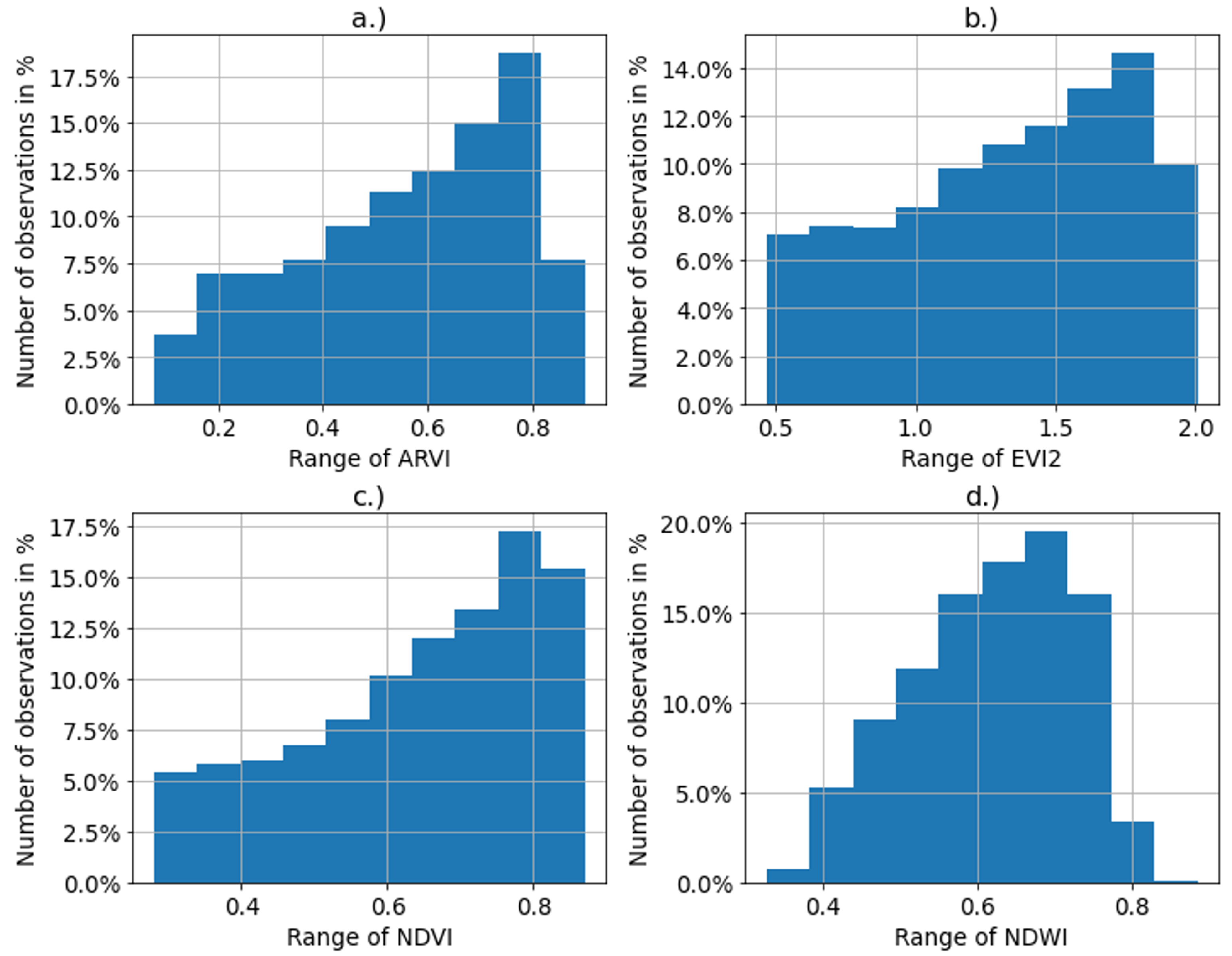
3.1. Extracted Features

A negative skew can be seen for the distributions of the ARVI, EVI2, NDVI, and NDWI (Figure 2). Only four of the 272 gathered features are analyzed and presented, since all other vegetation indices have similar characteristics and these VIs are the most common indices in the remote sensing field.

The negative skew can be explained by the time-filtered growth phase and the recording time, meaning that most cloud-free observations were collected in April and May, which correlates to the high reflectance values in Figure 3. In this growth phase, the reflection of the crops is highest with the appearance of silage maize, since this growth phase starts late (Figure 3). A similar reflectance behaviour can be observed between winter rye and winter wheat, as these plants are part of the Poaceae plant family. In addition, the entire growth phase of the plant from appearance to harvest can be observed. The cycle starts with the sowing season (September to October) and a subsequent growth phase over the winter into spring, with peak values in May and a subsequent harvest in June and July. A constant reflection characterizes agricultural grass throughout the year [40].

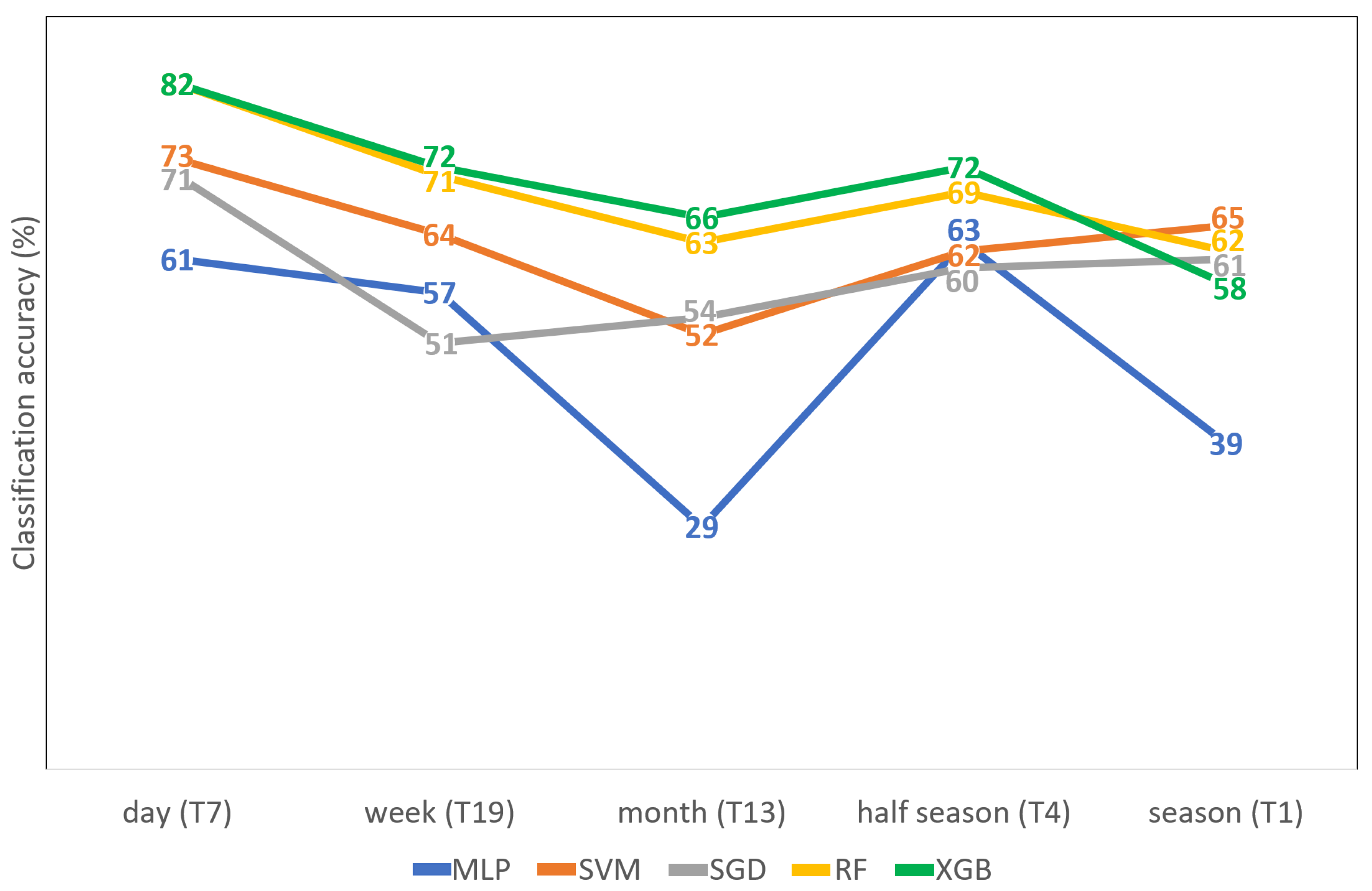
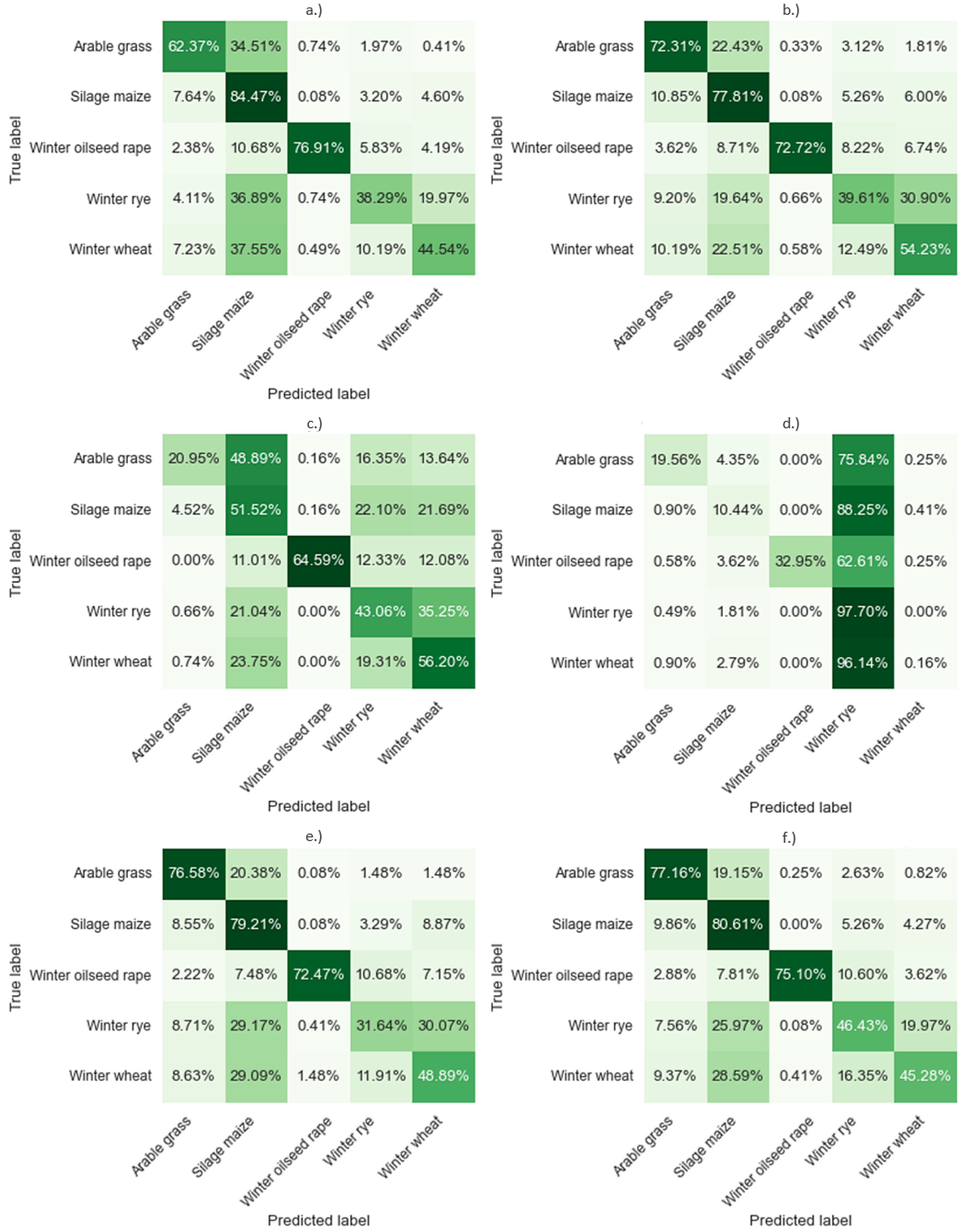
3.2. Interpretation of the Results

The reflectance characteristics of crops are subject to high variability due to environmental influences. Therefore, the data were divided into north and south regions to test the models based on the environmental variability in these regions. As shown in Figure 4, the accuracy tends to decrease with increasing period. This means that the models trained with a phenological mixed dataset (data from full growing season) had difficulties attributing the different growth phases to the plant species. Each period was trained in the north and tested in the south, since more observations are available in the north and, thus, the spectral diversity can be better represented in the model. The half-season shows a higher classification accuracy despite the increasing period. Studying the test cases T13 (

Table A6. The results for the test case T13 show the precision and recall of the XGBoost model on the validation dataset (north) and the test area (south).

	North			South
Crop	Precision (%)	Recall (%)	F1-Score (%)	Precision (%)	Recall (%)	F1-Score (%)
Agricultural grass	81	81	81	70	76	73
Silage maize	75	77	76	58	69	63
Winter rapeseed	94	92	93	94	79	86
Winter rye	71	70	70	57	53	55
Winter wheat	75	77	76	61	60	60

) and T15 (

Table A7. The results for the test case T15 show the precision and recall of the XGBoost model on the validation dataset (north) and the test area (south).

	North			South
Crop	Precision (%)	Recall (%)	F1-Score (%)	Precision (%)	Recall (%)	F1-Score (%)
Agricultural grass	82	90	86	78	92	84
Silage maize	93	90	91	94	74	83
Winter rapeseed	98	98	98	98	95	97
Winter rye	77	77	77	67	78	72
Winter wheat	83	78	81	74	64	69

), a high difference in the classification accuracy can be seen. This can be primarily attributed to the fact that the crop’s phenology, influenced by water availability, exhibits a more advanced phenological stage in May than in April, leading to a higher spectral response of the plant. Therefore, they can be better distinguished from each other in their reflection response (Figure 3). The development stage of the crops can explain the higher classification accuracy of the half-season (T4, training in April and May north/testing in April and May south), as the May data (T15, training in May north/testing in May south) in the half-season noticeably improves the overall classification. The large difference between the daily and seasonal data shows how big the phenological difference is between north and south (Figure 4).

For the investigations of the spatial and temporal influence of used training data on the trained models, the features are divided according to the northern and southern investigation areas. The collected observations are limited to the study period from 1 January 2018 to 16 July 2018, as all studied crops have already been harvested (Figure 3). For the year 2018, 26,359 observations were collected, with 66.84% (24,303) in the north and 33.16% (12,056) in the south. Apparent differences (Figure 2, skewness of −0.47, −0.33, −0.56, and −0.35) are noticeable in the distribution of the collected observations within the classes and between the different training areas. Figure 2 provides further explanations for the behavior of the models by investigating the skewness of the data in a histogram. Due to the indices’ negative skewness, many reflectances range within the vegetation spectrum because the most cloud-free observations could be collected in April and May. During these months, the vegetation reached a visually distinguishable growth phase, which aligns with the high classification accuracy in Figure 4 of the test case T4 (half-season). Thus, the classification’s temporal variability in accuracy can also be explained by investigating the distribution and skewness of the reflectances.

Figure 5 shows the confusion matrices for the tested models including Majority Voting. The models were trained in the north and applied to the test area in the south. For all models except the SGD method, the accuracies are highest for the arable grass, silage maize, and winter oilseed rape classes due to their biological differences. Winter rye and winter wheat, on the other hand, were more difficult to separate due to their similarity in phenology (Figure 3). In the transfer of the models, SGD performed worst, which could be due to an overfitting of the data. Thus, the SGD model is neither able to distinguish crops reliably nor to transfer them to other regions. However, all crops could best be distinguished from winter oilseed rape, which was to be expected due to the biologically conspicuous characteristics. Field grass was also well classified due to constant reflection during the growing season, but there was increasing confusion with silage maize in all models. The classification of silage maize was reliable in models XGBoost, Multilayer Perceptron, Random forest, and Majority Voting. It is noticeable that SVM is particularly well placed to separate winter rye and winter wheat from field grass but that all other crops were confused with winter rye and winter wheat. The Majority Vote led to an equalization of high and low scores, where high accuracy decreased and low accuracy increased. Majority Voting is the best transferability model, with a combined F1-score and an accuracy of 0.65. The results of all the trained models are presented in detail in

Table A1. Results for precision and recall of the validation dataset (north) and the test area (south) of the XGBoost model.

	North			South
Crop	Precision (%)	Recall (%)	F1-Score (%)	Precision (%)	Recall (%)	F1-Score (%)
Agricultural grass	81	89	85	74	62	68
Silage maize	81	83	82	41	84	56
Winter rapeseed	95	94	94	97	77	86
Winter rye	76	74	75	64	38	48
Winter wheat	82	76	79	60	45	51

,

Table A2. Results for precision and recall of the validation dataset (north) and the test area (south) of the Random Forest model.

	North			South
Crop	Precision (%)	Recall (%)	F1-Score (%)	Precision (%)	Recall (%)	F1-Score (%)
Agricultural grass	77	84	80	68	72	70
Silage maize	78	81	79	51	78	62
Winter rapeseed	97	90	93	98	73	83
Winter rye	68	73	70	58	40	47
Winter wheat	79	69	74	54	54	54

,

Table A3. Results for precision and recall of the validation dataset (north) and the test area (south) of the Support Vector Machine model.

	North			South
Crop	Precision (%)	Recall (%)	F1-Score (%)	Precision (%)	Recall (%)	F1-Score (%)
Agricultural grass	78	85	82	78	21	33
Silage maize	79	81	80	33	52	40
Winter rapeseed	96	93	95	99	65	78
Winter rye	75	73	74	38	43	40
Winter wheat	79	74	76	40	56	47

,

Table A4. Results for precision and recall of the validation dataset (north) and the test area (south) of the Stochastic Gradient Descent.

	North			South
Crop	Precision (%)	Recall (%)	F1-Score (%)	Precision (%)	Recall (%)	F1-Score (%)
Agricultural grass	78	81	80	87	20	32
Silage maize	80	68	74	45	10	17
Winter rapeseed	95	94	95	100	33	55
Winter rye	65	61	63	23	98	38
Winter wheat	63	74	68	15	0	0

and

Table A5. Results for precision and recall of the validation dataset (north) and the test area (south) of the Multilayer Perceptron model.

	North			South
Crop	Precision (%)	Recall (%)	F1-Score (%)	Precision (%)	Recall (%)	F1-Score (%)
Agricultural grass	82	85	83	73	77	75
Silage maize	78	76	77	48	79	60
Winter rapeseed	90	95	92	97	72	83
Winter rye	65	58	61	54	32	40
Winter wheat	66	69	67	51	49	50

. As shown in

Table 7. Results for precision and recall of the training dataset north (N) and the test area south (S) of the Majority Voting model for test case T10 (Table 6).

	Precision [72]			Recall [72]			F1-Score [72]
Crop	N	S	$\Delta$	N	S	$\Delta$	N	S	$\Delta$
	(%)	(%)	(%)	(%)	(%)	(%)	(%)	(%)	(%)
Agricultural grass	79	72	−8.86	88	77	−12.50	83	75	−9.63
Silage maize	82	50	−39.02	80	81	1.25	81	62	−23.45
Winter wheat	82	61	−25.60	75	45	−40.00	78	52	−33.33
Winter rye	75	57	−24.00	75	46	−38.66	75	51	−32.00
Winter rapeseed	95	99	4.21	93	75	−19.35	94	85	−9.57

, the classification precision and the recall of the models decreases when trained on the data of the northern test site and then transferred to the southern test site. The exceptions for which an improvement can be observed are winter rape in precision and silage maize in recall. Winter rape and arable grass are perfectly classifiable and transferable. Winter wheat and winter rye were difficult to distinguish and transfer for all models (Table 7).

4. Discussion

4.1. Environmental Influencing Factors

The results were also influenced by the extreme weather conditions of 2018. Between May and July, there is a slight dip in the reflection due to the drought called premature ripening (Figure 3). April 2018 was too warm and sunny compared to the climate reference value. The temperature differences at this time were notable, as daytime highs between 15 and 20 °C contrasted with nighttime lows near the frostline. Although the delayed vegetation development from May could be compensated and the values were mostly in the normal range, the growth was slowed due to the temperature differences between day and night. In May, sunshine was above average and reached 120% to 160% of the typical values with daily maximum temperatures up to 30 °C, so that May was too warm and too dry. Precipitation distribution was variable, reaching 20% to 70% compared to the 1981–2010 long-term average. Low precipitation, high evaporation rates, and a soil temperature of around 20 °C in the upper layers severely dried out the topsoil. For the third month in a row, June was too warm. In many places, the sunny weather caused a further tense situation concerning the water supply for crops [41]. Thus, the crops were exposed to heat and water stress, affecting the classification results and the transferability as well.

4.2. Classification Results

The models can differentiate well between biologically different crops due to plant-specific reflection and natural and unnatural vegetation due to the constant reflection behavior of natural crops (Figure 3). Differentiating between similar crops like wheat and rye is more complicated. For these similar crops, the classification results were lower and the confusion was higher (Figure 5). The results show that regionally temporally different phenological developments influence spectral characteristics and, thus, also the classification accuracy. Spectral analyses have shown that in the different regions, the phenological phases differ in start time and length (Figure 3). The training results are comparable to those from other studies and range between 75% and 94% [7,54,73], depending on the crop type and the location (Table 7). The models seem to specialize rather than generalize to perform with the best classification accuracy possible, so parameters must be adjusted for generalization. Furthermore, the processor classifies per field, not per pixel, in which the pixel values are aggregated within the field. Field-based classification has advantages in reduced computation times, and no polygon detection is needed to derive the features per field. In order to ensure a reliable crop classification, sufficient cloud-free observations must represent spectral diversity in the model.

4.3. Systematic Approach of the Testing Methodology

Referring back to the literature review, while the problems of transferability are known, they have not been systematically analyzed [24,25,27,28,29,30]. Using the testing methodology presented here (Table 6), spatial transferability problems can now be systematically investigated in hopes of gaining insight into the causes and effects of transferability. Table 6 provides information on the quality of the spatial transfer of trained machine learning models (Figure 4), which is accomplished by including space, time, and the associated different phenological growth phases as parameters (Table 6). As similar studies also found [74], simple training on the entire data set is not sufficient to ensure the transferability of the model to other regions, and the classification accuracy varies significantly when models are trained in different regions [75]. The benefit of this method is that it is a systematic approach, meaning it can be used regardless of any machine learning model that classifies crops. The test methodology allows for the validation and estimation of the crop classification performance for various machine learning models. The presented testing methodology allows for conclusions on the model’s generalization capabilities and phenological, temporal, spatial, and quantitative influences to be drawn.

5. Conclusions

This research aimed to investigate the transferability of machine learning models for crop classification by using a new testing methodology. The methodology systematically analyzes the quality of the spatial transfer of trained models (and, thus, the transferability of the developed models to new application areas) to other test areas that differ from the training areas in terms of topography and climatic characteristics (Table 1). It is shown that the new testing methodology can be a reliable strategy to assess the applicability of machine learning models in crop classification for application in new regions. The results show that the models cannot be transferred to other areas without adaptation. The accuracy of the classification results decreased when the training took place in the respective opposite test areas (e.g., training in the south) and when the trained methods were applied to the respective opposite test area (e.g., application in the north). Furthermore, the accuracies tended to decrease with increasing period. The combined F1-score was 82% (XGBoost) when trained on a single day, 72% (XGBoost) when trained on the half-season, and 61% when trained over the entire growing season (Majority Voting) (Figure 4).

The testing methodology was developed to combine temporal and regional test cases, enabling the identification of potential phenological, temporal, spatial, and quantitative influences. The study area of Brandenburg was selected because it can be divided into two test areas with differing geographies (Figure 1). Environmental factors such as phenology, soil deposition, and groundwater can be expected to influence the transferability of machine learning models (Table 1). The research clearly illustrates that the classification accuracy decreases when the training and testing occur in opposite locations (Table 7). The question arises as to whether machine learning models can account for variations in environmental factors or if their performance may be limited in regions with similar environmental conditions. Although they may achieve high classification accuracy, their transferability to other areas may be low.

To develop transferable models and better understand their implications, it is essential to have sufficient heterogeneous in situ data from various study areas in terms of both quality and quantity. Analyzing weaknesses within models is only possible if large and heterogeneous study areas are selected for investigation, which is in turn related to the availability of reliable in situ data and, therefore, could be a limiting factor. Future studies should investigate the influence of a systematic sampling strategy on local spectral diversity. Additionally, future studies should explore the extent to which a universally applicable model-fixing approach can be developed.

This research contributes to the development of more efficient and accurate methods for crop monitoring and inventory, which are essential for ensuring food security in a growing global population, by introducing a new test strategy. This study addressed the knowledge gap regarding the consequences of transferring a model to different regions by providing a systematic testing methodology that offers insights into quantitative, spatial, and temporal conditions.

References

1. United Nations. World Population Prospects 2017: Data Booklet; United Nations, Department of Economic and Social Affairs: New York, NY, USA, 2017. [Google Scholar]
2. Tuomisto, H.; Scheelbeek, P.; Chalabi, Z.; Green, R.; Smith, R.; Haines, A.; Dangour, A. Effects of environmental change on agriculture, nutrition and health: A framework with a focus on fruits and vegetables. Wellcome Open Res. 2017, 2, 21. [Google Scholar] [CrossRef] [PubMed]
3. Shankar, T.; Praharaj, S.; Sahoo, U.; Maitra, S. Intensive Farming: It’s Effect on the Environment. Int. Bimon. 2021, 12, 37480–37487. [Google Scholar]
4. Funk, R.; Völker, L.; Deumlich, D. Landscape structure model based estimation of the wind erosion risk in Brandenburg, Germany. Aeolian Res. 2023, 62, 100878. [Google Scholar] [CrossRef]
5. SUHET. Sentinel-2, User Handbook, 1st ed.; European Space Agency (ESA): Paris, France, 2013. [Google Scholar]
6. Woodcock, C.; Allen, R.; Anderson, M.; Belward, A.; Bindschadler, R.; Cohen, W.; Gao, F.; Goward, S.; Helder, D.; Helmer, E.; et al. Free Access to Landsat Imagery. Science 2008, 320, 1011. [Google Scholar] [CrossRef] [PubMed]
7. Blickensdörfer, L.; Schwieder, M.; Pflugmacher, D.; Nendel, C.; Erasmi, S.; Hostert, P. Mapping of crop types and crop sequences with combined time series of Sentinel-1, Sentinel-2 and Landsat 8 data for Germany. Remote Sens. Environ. 2022, 269, 112831. [Google Scholar] [CrossRef]
8. Waldhoff, G.; Lussem, U.; Bareth, G. Multi-Data Approach for remote sensing-based regional crop rotation mapping: A case study for the Rur catchment, Germany. Int. J. Appl. Earth Obs. Geoinf. 2017, 61, 55–69. [Google Scholar] [CrossRef]
9. Muruganantham, P.; Wibowo, S.; Grandhi, S.; Samrat, N.H.; Islam, N. A Systematic Literature Review on Crop Yield Prediction with Deep Learning and Remote Sensing. Remote Sens. 2022, 14, 1990. [Google Scholar] [CrossRef]
10. Gao, Q.; Zribi, M.; Escorihuela, M.J.; Baghdadi, N.; Segui, P.Q. Irrigation Mapping Using Sentinel-1 Time Series at Field Scale. Remote Sens. 2018, 10, 1495. [Google Scholar] [CrossRef]
11. Santaga, F.S.; Benincasa, P.; Toscano, P.; Antognelli, S.; Ranieri, E.; Vizzari, M. Simplified and Advanced Sentinel-2-Based Precision Nitrogen Management of Wheat. Agronomy 2021, 11, 1156. [Google Scholar] [CrossRef]
12. Berger, M.; Moreno, J.; Johannessen, J.A.; Levelt, P.F.; Hanssen, R.F. ESA’s sentinel missions in support of Earth system science. Remote Sens. Environ. 2012, 120, 84–90. [Google Scholar] [CrossRef]
13. Thompson, N.C.; Ge, S.; Manso, G.F. The Importance of (Exponentially More) Computing Power. In Proceedings of the Academy of Management Annual Meeting Proceedings, Seattle, DC, USA, 5–9 August 2022. [Google Scholar]
14. Molas, G.; Nowak, E. Advances in Emerging Memory Technologies: From Data Storage to Artificial Intelligence. Appl. Sci. 2021, 11, 11254. [Google Scholar] [CrossRef]
15. Capra, M.; Bussolino, B.; Marchisio, A.; Masera, G.; Martina, M.; Shafique, M. Hardware and Software Optimizations for Accelerating Deep Neural Networks: Survey of Current Trends, Challenges, and the Road Ahead. IEEE Access 2020, 8, 225134–225180. [Google Scholar] [CrossRef]
16. Lu, T.; Gao, M.; Wang, L. Crop classification in high-resolution remote sensing images based on multi-scale feature fusion semantic segmentation model. Front. Plant Sci. 2023, 14, 1196634. [Google Scholar] [CrossRef] [PubMed]
17. Li, Q.; Tian, J.; Tian, Q. Deep Learning Application for Crop Classification via Multi-Temporal Remote Sensing Images. Agriculture 2023, 13, 906. [Google Scholar] [CrossRef]
18. Kang, J.; Zhang, H.; Yang, H.; Zhang, L. Support Vector Machine Classification of Crop Lands Using Sentinel-2 Imagery. In Proceedings of the 2018 7th International Conference on Agro-Geoinformatics (Agro-Geoinformatics), Hangzhou, China, 6–9 August 2018; pp. 1–6. [Google Scholar] [CrossRef]
19. Ok, A. Evaluation of random forest method for agricultural crop classification. Eur. J. Remote Sens. 2012, 45, 421–432. [Google Scholar] [CrossRef]
20. Saini, R.; Ghosh, S.K. Crop Classification on Single Date SENTINEL-2 Imagery Using Random Forest and Suppor Vector Machine. ISPRS Int. Arch. Photogramm. Remote Sens. Spat. Inf. Sci. 2018, 425, 683–688. [Google Scholar] [CrossRef]
21. Rodriguez-Galiano, V.; Ghimire, B.; Rogan, J.; Chica-Olmo, M.; Rigol-Sanchez, J. An assessment of the effectiveness of a random forest classifier for land-cover classification. ISPRS J. Photogramm. Remote Sens. 2012, 67, 93–104. [Google Scholar] [CrossRef]
22. Song, Q.; Hu, Q.; Zhou, Q.; Hovis, C.; Xiang, M.; Tang, H.; Wu, W. In-Season Crop Mapping with GF-1/WFV Data by Combining Object-Based Image Analysis and Random Forest. Remote Sens. 2017, 9, 1184. [Google Scholar] [CrossRef]
23. Skriver, H.; Mattia, F.; Satalino, G.; Balenzano, A.; Pauwels, V.; Verhoest, N.; Davidson, M. Crop Classification Using Short-Revisit Multitemporal SAR Data. IEEE J. Sel. Top. Appl. Earth Obs. Remote Sens. 2011, 4, 423–431. [Google Scholar] [CrossRef]
24. Orynbaikyzy, A.; Gessner, U.; Conrad, C. Spatial Transferability of Random Forest Models for Crop Type Classification Using Sentinel-1 and Sentinel-2. Remote Sens. 2022, 14, 1493. [Google Scholar] [CrossRef]
25. Rusňák, T.; Kasanický, T.; Malík, P.; Mojžiš, J.; Zelenka, J.; Sviček, M.; Abrahám, D.; Halabuk, A. Crop Mapping without Labels: Investigating Temporal and Spatial Transferability of Crop Classification Models Using a 5-Year Sentinel-2 Series and Machine Learning. Remote Sens. 2023, 15, 3414. [Google Scholar] [CrossRef]
26. Luo, Y.; Zhang, Z.; Zhang, L.; Han, J.; Cao, J.; Zhang, J. Developing High-Resolution Crop Maps for Major Crops in the European Union Based on Transductive Transfer Learning and Limited Ground Data. Remote Sens. 2022, 14, 1809. [Google Scholar] [CrossRef]
27. Ge, S.; Zhang, J.; Pan, Y.; Yang, Z.; Zhu, S. Transferable deep learning model based on the phenological matching principle for mapping crop extent. Int. J. Appl. Earth Obs. Geoinf. 2021, 102, 102451. [Google Scholar] [CrossRef]
28. Wenger, S.J.; Olden, J.D. Assessing transferability of ecological models: An underappreciated aspect of statistical validation. Methods Ecol. Evol. 2012, 3, 260–267. [Google Scholar] [CrossRef]
29. Roberts, D.; Bahn, V.; Ciuti, S.; Boyce, M.; Elith, J.; Guillera-Arroita, G.; Hauenstein, S.; Lahoz-Monfort, J.; Schröder, B.; Thuiller, W.; et al. Cross-validation strategies for data with temporal, spatial, hierarchical, or phylogenetic structure. Ecography 2016, 40, 913–929. [Google Scholar] [CrossRef]
30. Löw, F.; Michel, U.; Dech, S.; Conrad, C. Impact of feature selection on the accuracy and spatial uncertainty of per-field crop classification using Support Vector Machines. ISPRS J. Photogramm. Remote Sens. 2013, 85, 102–119. [Google Scholar] [CrossRef]
31. Wang, S.; Azzari, G.; Lobell, D.B. Crop type mapping without field-level labels: Random forest transfer and unsupervised clustering techniques. Remote Sens. Environ. 2019, 222, 303–317. [Google Scholar] [CrossRef]
32. Bundesamt, S. (Ed.) Statistisches Jahrbuch; Amt für Statistik Berlin-Brandenburg: Wiesbaden, Germany, 2020. [Google Scholar]
33. Klima & Gjennomsnittsvær i Cottbus, Brandenburg, Tyskland. Available online: https://www.timeanddate.no/vaer/tyskland/cottbus/klima (accessed on 28 September 2023).
34. Wendel, M. Das Klima Norddeutschlands; VerlagGRIN Verlag: Munich, Germany, 2007; p. 29. [Google Scholar]
35. Gerstengarbe, F.; Badeck, F.W.; Hattermann, F.; Krysanova, V.; Lahmer, W.; Lasch, P.; Stock, M.; Suckow, F.; Wechsung, F.; Werner, P. Studie zur Klimatischen Entwicklung im Land Brandenburg bis 2055 und 55 deren Auswirkungen auf den Wasserhaushalt, Die Forst- und Landwirtschaft Sowie Die Ableitung Erster Perspektive; Ministerium für Landwirtschaft, Umwelt und Klimaschutz des Landes Brandenburg: Potsdam, Germany, 2003; Volume 83, p. 96. [Google Scholar]
36. Stackebrandt, W. Atlas zur Geologie von Brandenburg: Im Maßstab 1:1,000,000; Landesamt für Bergbau, Geologie und Rohstoffe Brandenburg: Cottbus, Germany, 2010. [Google Scholar]
37. Remy, T.H.D. Jahrestagung der Floristisch-Soziologischen Arbeitsgemeinschaft (FlorSoz) in Potsdam 2011; Tuexenia: Potsdam, Germany, 2011. [Google Scholar]
38. Hofmann, G.; Pommer, U. Potentielle Natürliche Vegetation von Brandenburg und Berlin: Mit Karte im Maßstab 1:200,000; Eberswalder Forstliche Schriftenreihe, Ministerium für Ländliche Entwicklung, Umwelt und Verbraucherschutz des Landes Brandenburg, Referat Presse- und Öffentlichkeitsarbeit; Ministry of Rural Development, Environment and Consumer Protection: Potsdam, Germany, 2005. [Google Scholar]
39. Theuerkauf, M. Younger Dryas cold stage vegetation patterns of central Europe—Climate, soil and relief controls. Boreas 2012, 41, 391–407. [Google Scholar] [CrossRef]
40. Hoppe, H. Crop Type Classification in the Federal State Brandenburg Using Machine Learning Models and Multi-Temporal, Multispectral Sentinel-2 Imagery. Master’s Thesis, Stralsund University of Applied Sciences, Faculty of Economics, Stralsund, Germany, 2021. [Google Scholar]
41. Amt für Statistik Berlin-Brandenburg. Statistischer Bericht C II 7– j/18—Besondere Ernte- und Qualitätsermittlung im Land Brandenburg 2018; Statistik Berlin Brandenburg: Potsdam, Germany, 2019. [Google Scholar]
42. Louis, J.; Debaecker, V.; Pflug, B.; Main-Knorn, M.; Bieniarz, J.; Mueller-Wilm, U.; Cadau, E.; Gascon, F. SENTINEL-2 SEN2COR: L2A Processor for Users. In Proceedings of the Proceedings Living Planet Symposium 2016, Prague, Czech Republic, 9–13 May 2016; Spacebooks Online. Ouwehand, L., Ed.; ESA Special Publications (on CD). 2016; Volume SP-740, pp. 1–8. [Google Scholar]
43. Oehmichen, G. Auf Satellitendaten basierende Ableitungen von Parametern zur Beschreibung Terrestrischer Ökosysteme: Methodische Untersuchung zur Ableitung der Chlorophyll(a+b)- Konzentration und des Blattflächenindexes aus Fernerkundungsdaten. UFO Dissertation, UFO, Atelier für Gestaltung und Verlag, Hamburg, Germany, 2004. [Google Scholar]
44. Witt, H. Die Spektralen und Räumlichen Eigenschaften von Fernerkundungssensoren bei der Ableitung von Landoberflächenparametern; Technical Report; Institut für Planetenforschung; Institut für Weltraumsensorik: Berlin, Germany, 1998; Institut für Planetenforschung. [Google Scholar]
45. Ministerium für Landwirtschaft, Umwelt und Klimaschutz des Landes Brandenburg. GEOBROKER der Internetshop der LGB. Agrarantragsdaten—Produktmetadaten Geobroker–Der Internetshop der LGB. Available online: https://geobroker.geobasis-bb.de/gbss.php?MODE=GetProductInformation&PRODUCTID=996f8fd1-c662-4975-b680-3b611fcb5d1f (accessed on 6 June 2022).
46. Kaufman, Y.; Tanre, D. Atmospherically resistant vegetation index (ARVI) for EOS-MODIS. IEEE Trans. Geosci. Remote Sens. 1992, 30, 261–270. [Google Scholar] [CrossRef]
47. Jiang, Z.; Huete, A.R.; Didan, K.; Miura, T. Development of a two-band enhanced vegetation index without a blue band. Remote Sens. Environ. 2008, 112, 3833–3845. [Google Scholar] [CrossRef]
48. Frampton, W.J.; Dash, J.; Watmough, G.R.; Milton, E.J. Evaluating the capabilities of Sentinel-2 for quantitative estimation of biophysical variables in vegetation. ISPRS J. Photogramm. Remote Sens. 2013, 82, 83–92. [Google Scholar] [CrossRef]
49. Rouse, J.W.; Haas, R.H.; Deering, D.W.; Schell, J.A.; Harlan, J.C. Monitoring the Vernal Advancement and Retrogradation (Green Wave Effect) of Natural Vegetation. [Great Plains Corridor]. In Proceedings of the Monitoring the Vernal Advancement and Retrogradation (Green Wave Effect) of Natural Vegetation. [Great Plains Corridor], College Station, TX, USA, 27 January 1973. [Google Scholar]
50. McFeeters, S.K. The use of the Normalized Difference Water Index (NDWI) in the delineation of open water features. Int. J. Remote Sens. 1996, 17, 1425–1432. [Google Scholar] [CrossRef]
51. Birth, G.S.; Mcvey, G.R. Measuring the Color of Growing Turf with a Reflectance Spectrophotometer1. Agron. J. 1968, 60, 640–643. [Google Scholar] [CrossRef]
52. Kang, Y.; Hu, X.; Meng, Q.; Zou, Y.; Zhang, L.; Liu, M.; Zhao, M. Land Cover and Crop Classification Based on Red Edge Indices Features of GF-6 WFV Time Series Data. Remote Sens. 2021, 13, 4522. [Google Scholar] [CrossRef]
53. Orynbaikyzy, A.; Gessner, U.; Mack, B.; Conrad, C. Crop Type Classification Using Fusion of Sentinel-1 and Sentinel-2 Data: Assessing the Impact of Feature Selection, Optical Data Availability, and Parcel Sizes on the Accuracies. Remote Sens. 2020, 12, 2779. [Google Scholar] [CrossRef]
54. Wang, L.; Wang, J.; Liu, Z.; Zhu, J.; Qin, F. Evaluation of a deep-learning model for multispectral remote sensing of land use and crop classification. Crop J. 2022, 10, 1435–1451. [Google Scholar] [CrossRef]
55. OpenCV. OpenCV: Clustering. Available online: https://docs.opencv.org/4.x/d5/d38/group__core__cluster.html#ga9a34dc06c6ec9460e90860f15bcd2f88 (accessed on 28 June 2022).
56. Breiman, L. Random Forests. Mach. Learn. 2001, 45, 5–32. [Google Scholar] [CrossRef]
57. Friedman, J.H. Greedy Function Approximation: A Gradient Boosting Machine. Ann. Stat. 2000, 29, 1189–1232. [Google Scholar] [CrossRef]
58. Chen, T.; Guestrin, C. XGBoost: A Scalable Tree Boosting System. arXiv 2016, arXiv:1603.02754. [Google Scholar] [CrossRef]
59. Cortes, C.; Vapnik, V. Support Vector Networks. Mach. Learn. 1995, 20, 273–297. [Google Scholar] [CrossRef]
60. von der Malsburg, C. Frank Rosenblatt: Principles of Neurodynamics: Perceptrons and the Theory of Brain Mechanisms. In Brain Theory; Springer: Berlin/Heidelberg, Germany, 1986; pp. 245–248. [Google Scholar] [CrossRef]
61. Anaconda Inc. Anaconda Software Distribution; Anaconda, Inc.: Austin, TX, USA, 2020. [Google Scholar]
62. QGIS Development Team. QGIS Geographic Information System; Open Source Geospatial Foundation: Beaverton, OR, USA, 2009. [Google Scholar]
63. Microsoft Corporation. Microsoft Excel; Microsoft Corporation: Redmond, WA, USA.
64. Harris, C.R.; Millman, K.J.; van der Walt, S.J.; Gommers, R.; Virtanen, P.; Cournapeau, D.; Wieser, E.; Taylor, J.; Berg, S.; Smith, N.J.; et al. Array programming with NumPy. Nature 2020, 585, 357–362. [Google Scholar] [CrossRef] [PubMed]
65. Virtanen, P.; Gommers, R.; Oliphant, T.E.; Haberland, M.; Reddy, T.; Cournapeau, D.; Burovski, E.; Peterson, P.; Weckesser, W.; Bright, J.; et al. SciPy 1.0: Fundamental Algorithms for Scientific Computing in Python. Nat. Methods 2020, 17, 261–272. [Google Scholar] [CrossRef] [PubMed]
66. Hunter, J.D. Matplotlib: A 2D graphics environment. Comput. Sci. Eng. 2007, 9, 90–95. [Google Scholar] [CrossRef]
67. The Pandas Development Team. pandas-dev/pandas: Pandas 2020. [CrossRef]
68. Pedregosa, F.; Varoquaux, G.; Gramfort, A.; Michel, V.; Thirion, B.; Grisel, O.; Blondel, M.; Prettenhofer, P.; Weiss, R.; Dubourg, V.; et al. Scikit-learn: Machine learning in Python. J. Mach. Learn. Res. 2011, 12, 2825–2830. [Google Scholar]
69. Haralick, R.M.; Shanmugam, K.; Dinstein, I. Textural Features for Image Classification. IEEE Trans. Syst. Man Cybern. 1973, SMC-3, 610–621. [Google Scholar] [CrossRef]
70. Kühn, D.; Auriegel, A.; Müller, H.; Rosskopf, N. Charakterisierung der Böden Brandenburgs Hinsichtlich Ihrer Verbreitung, Eigenschaften und Potenziale mit Einer Präsentation Gemittelter Analytischer Untersuchungsergebnisse Einschließlich von Hintergrundwerten (Korngrößenzusammensetzung, Bodenphysik, Bodenchemie); Brandenburger Geowissenschaftliche Beiträge: Cottbus, Germany, 2015. [Google Scholar]
71. Peña, J.M.; Gutiérrez, P.A.; Hervás-Martínez, C.; Six, J.; Plant, R.E.; López-Granados, F. Object-Based Image Classification of Summer Crops with Machine Learning Methods. Remote Sens. 2014, 6, 5019–5041. [Google Scholar] [CrossRef]
72. Goutte, C.; Gaussier, E. A Probabilistic Interpretation of Precision, Recall and F-Score, with Implication for Evaluation. In Proceedings of the Probabilistic Interpretation of Precision, Recall and F-Score, with Implication for Evaluation, 04, Santiago de Compostela, Spain, 21–23 March 2005; Volume 3408, pp. 345–359. [Google Scholar] [CrossRef]
73. Saini, R.; Ghosh, S.K. Crop classification in a heterogeneous agricultural environment using ensemble classifiers and single-date Sentinel-2A imagery. Geocarto Int. 2021, 36, 2141–2159. [Google Scholar] [CrossRef]
74. Wijesingha, J.; Dzene, I.; Wachendorf, M. Spatial-temporal transferability assessment of remote sensing data models for mapping agricultural land use. In Proceedings of the Spatial-Temporal Transferability Assessment of Remote Sensing Data Models for Mapping Agricultural Land Use, 04, Vienna, Austria, 24–28 April 2023. [Google Scholar] [CrossRef]
75. Arias, M.; Campo-Bescós, M.A.; Álvarez Mozos, J. Crop Classification Based on Temporal Signatures of Sentinel-1 Observations over Navarre Province, Spain. Remote Sens. 2020, 12, 278. [Google Scholar] [CrossRef]
76. Agency, E.S. Copernicus Open Access Hub. Available online: https://scihub.copernicus.eu/ (accessed on 6 June 2022).
Figure 1. Pink are the crop fields for training and yellow are the crop fields for validation. The intersecting part (black) was removed from the training and validation set (adapted and modified from [40]).
Remotesensing 16 01493 g001
Figure 2. Distribution of data collected for all crops with VIs aggregated over the growth period. Skewness: (a) ARVI: −0.47, (b) EVI2: −0.33, (c) NDVI: −0.56, and (d) NDWI: −0.35 (adapted and modified from [40]).
Remotesensing 16 01493 g002
Figure 3. Growth phase shown by the NDVI over the total period from sowing to harvest for each field crop. For illustration purposes, a four-day interval was used.
Remotesensing 16 01493 g003
Figure 4. F1-score (metric that measures accuracy by combining precision and recall [72]) of all trained models over the different time periods T (Table 6).
Remotesensing 16 01493 g004
Figure 5. Confusion matrices for test case T10 (Table 6) of all models trained in the north and applied to the new region in the south that were not included in the training data: (a) XGBoost (Table A1), (b) Random Forest (Table A2), (c) Support Vector Machine (Table A3), (d) Stochastic Gradient Descent (Table A4), (e) Multilayer Perceptron (Table A5), (f) Majority Voting (Table 7).
Remotesensing 16 01493 g005