Adaptive Resource Scheduling Algorithm for Multi-Target ISAR Imaging in Radar Systems

Abstract

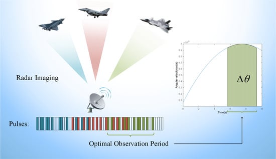
Inverse synthetic-aperture radar (ISAR) can achieve precise imaging of targets, which enables precise perception of battlefield information, and it has become one of the most important tasks for radar systems. In multi-target scenarios, a resource scheduling method is required to improve the sensing ability and the overall efficiency of a radar system due to the limited resources. Considering the motion state of the target will change as the observation distance increases and image defocusing can occur due to the prolonged coherence accumulation time and significant changes in the target’s motion state, the optimal observation period should be an important consideration factor in the resource scheduling method to further improve the imaging efficiency of radar system, which has not yet been involved in existing research. In this paper, we first derive the expressions of the target’s effective rotation angle and the equivalent rotation angular velocity and then define the target’s optimal observation period. Then, for multi-target imaging scenarios, we allocate pulse resources within a given time period based on sparse-aperture ISAR imaging technology. An adaptive radar resource scheduling algorithm for multi-target ISAR imaging is proposed, which prioritizes allocating resources based on the optimal observation periods for the targets. In the algorithm, a radar resource scheduling model for multi-target ISAR imaging is established, and a feedback-based closed-loop search optimization method is proposed to solve the model. Finally, the best scheduling strategy can be obtained, which includes imaging task duration and the pulse allocation sequence for each target. Simulation results validate the effectiveness of the algorithm.

1. Introduction

Inverse synthetic-aperture radar (ISAR) imaging technology is the use of ground-based radar to detect and image moving aerial and spaceborne targets, which enables the capture of detailed characteristics of the targets, such as dimensions and geometry, and is of wide value in the military and civil domains. Unlike optical imaging systems, radars can operate effectively under adverse weather conditions like clouds and fog, and they can also provide additional information on the range dimension. Therefore, target imaging has become one of the most important tasks of radar systems [1,2,3].

ISAR imaging technology achieves high resolution in the range direction by transmitting signals with a large time-bandwidth product and achieves high resolution in the azimuth direction by forming a large synthetic aperture through the relative motion between the radar and the target, thereby obtaining high-resolution two-dimensional images. Radar range resolution is primarily determined by the bandwidth of the transmitted signal, while azimuth resolution depends on the relative rotation angle between the radar and the target [4]. In order to achieve a higher azimuth resolution, radar often requires prolonged continuous observation of the target, which means consuming more time resources [5]. However, radar resources are often limited. In multi-target scenarios, a reasonable and effective radar resource scheduling algorithm will allocate radar resources appropriately, thereby effectively enhancing the overall performance of the radar system [6,7,8,9,10,11,12,13].

Several research teams have explored diverse radar resource scheduling methods for imaging tasks, each contributing to improved radar system performance. Reference [14] first studied a radar resource scheduling problem for imaging tasks based on sparse-aperture ISAR imaging technology. By efficiently alternating observations of different targets, it simultaneously imaged multiple targets within a period of time, significantly improving imaging efficiency. On this basis, Reference [15] introduced the pulse interleaving technique into the resource scheduling process. The utilization rate of radar system resources is further improved by effectively utilizing the time resources of pulse waiting periods. Reference [16] combined pulse interleaving with pre-allocation strategies to avoid pulse conflicts and enable adaptive scheduling of radar time resources. Additionally, Reference [17] introduced aperture segmentation technology to jointly allocate radar time and aperture resources. Reference [18] leveraged multiple-input multiple-output (MIMO) phased array radar technology for multi-target imaging, optimizing array elements, power, and frequency resources to achieve enhanced efficiency. Moreover, for the networked radar imaging resource scheduling problem, Reference [19] investigated the resource scheduling problem of distributed MIMO radar for multi-target imaging and solved the problem based on maximizing scheduling benefits. Furthermore, Reference [20] defined a cooperative game-theoretic framework for task assignment optimization in radar network multi-target imaging, achieving efficient distribution and scheduling of radar nodes to minimize total imaging duration. However, it is important to note that most existing research in this area assumes that the motion state of the target remains unchanged during the observation period, whereas, as the observation distance increases and the observation time lengthens, the motion state of the target will change during the observation period. Additionally, dynamic changes in the target motion state will directly impact the imaging quality and the coherent accumulation time for imaging, thereby further influencing the resource scheduling strategy in multi-target scenarios.

When dealing with targets exhibiting changing motion states, it becomes crucial to select an optimal observation period based on state prediction results from target tracking. As we all know, higher angular velocity in the relative rotation between the radar and the target results in shorter coherent accumulation time for imaging, leading to reduced consumption of radar resources. In addition, when the target motion is smooth, the Doppler information generated by the target echo is basically unchanged, facilitating better imaging results when employing range-Doppler (RD) algorithms [21,22]. However, it is important to note that prolonged coherence accumulation time or significant changes in target motion states can lead to image defocusing [23,24,25]. Therefore, the selection of the optimal observation period directly affects both the coherence accumulation time and the performance of target imaging, and the radar resource scheduling algorithms that consider the optimal observation periods will further enhance the imaging efficiency of the radar system.

In one of the working modes of a multifunction phased array radar, a certain amount of time is often allocated for an imaging task, which is called imaging task duration. To enhance the flexibility of resource allocation, a sparse-aperture ISAR imaging algorithm is employed for target imaging, transforming continuous observation into sparse-aperture observation. This involves transmitting only a subset of pulses during selected observation periods and then using a signal reconstruction algorithm at the receiver side to recover the complete signal for target imaging [26]. Based on this sparsifiability property, the radar can achieve imaging of multiple targets simultaneously within the same period of time. Therefore, it is necessary to study how to allocate pulse resources to each target within the imaging task duration, using as few resources as possible to image as many targets as possible. Based on the aforementioned considerations and analysis, an adaptive radar resource scheduling method for multi-target ISAR imaging based on optimal observation periods is proposed. After we derive the expressions of the target’s effective rotation angle and equivalent rotation angular velocity, we define and calculate each target’s optimal observation period. Then, a resource scheduling model is constructed, with the imaging task duration and the pulse allocation sequence for each target being optimization variables, and a feedback-based closed-loop search optimization method is proposed to solve the model. By solving this model, the optimal scheduling strategy (including the imaging task duration and the pulse allocation sequence for each target) that satisfies various system performance indices can be obtained.

The paper is structured as follows. Section 2 introduces the main methods proposed in this paper, which include the formulation of the optimal observation period, the construction of the resource scheduling model, and the algorithm for model solving. In Section 3, the effectiveness of the algorithm is verified through simulation experiments. Finally, Section 4 provides the conclusion.

2. Materials and Methods

Aiming to address the problems of insufficient resources and low imaging efficiency when imaging multiple targets by radar, this paper proposes an adaptive radar resource scheduling algorithm for multi-target imaging based on optimal observation periods. The principle of sparse-aperture ISAR imaging technology is introduced first. Subsequently, the expressions of the target’s effective rotation angle and the equivalent rotation angular velocity are derived, and the target’s optimal observation period is defined. The algorithm then incorporates various constraints to construct the resource scheduling model based on optimal observation periods. Finally, a feedback-based closed-loop search optimization method is applied to solve the model and derive the optimal scheduling strategy.

2.1. Sparse-Aperture ISAR Imaging Principle

When observing a target, inverse synthetic-aperture radar can categorize the target’s relative motion into three types: circular motion around the radar, translational motion, and rotation around its own axis [27,28]. Circular motion around the radar results in a consistent motion state for the target. Translational motion refers to movement along the radar’s line of sight, resulting in uniform Doppler shifts across all scattering points, which do not contribute to the imaging. Thus, after compensating for any translational component through appropriate signal processing techniques, ISAR imaging focuses on isolating and analyzing the rotational component of the target’s motion to synthesize images as if observing a purely rotating object.

Based on the derivation, the Doppler frequency of the echo signal from each scatter point in the rotating target is $f_d=\frac{2v_p}{\lambda }=\frac{2\omega }{\lambda }{x}_p$, where $v_p$ denotes radial velocity relative to radar line of sight, $\lambda$ is the wavelength of the transmitted signal, $\omega$ is the target’s equivalent rotational angular velocity, and $x_p$ represents cross-range distance from the rotation axis to the scatter point. Therefore, it is possible to extract cross-range distance information of a target from the Doppler frequency of echoes from target scatter points. As long as the Doppler resolution is high enough, it can represent the cross-range distribution of the target; this ability forms the basic principle behind RD algorithm imaging. According to the theoretical derivation, radar azimuth resolution is intrinsically related to a target’s effective rotation angle relative to radar. For uniform rotational motion, this can be expressed as:

$${\rho }_a=\frac{\lambda }{2\mathsf{\Delta }\theta }=\frac{\lambda }{2\omega T_c},$$

(1)

where $\mathsf{\Delta }\theta$ is the target’s effective rotation angle, and $T_c$ is the coherent accumulation time required for target imaging. When accounting for changes in a target’s equivalent rotational angular velocity, the radar azimuth resolution can be expressed as:

$${\rho }_a=\frac{\lambda }{2\mathsf{\Delta }\theta }=\frac{\lambda }{2{\int }_{t_0}^{t_0+T_c}\omega \left(t\right)dt},$$

(2)

where $\omega \left(t\right)$ represents the time-varying equivalent rotational angular velocity, and $t_0$ is the starting moment of imaging.

The range resolution of radar is usually determined by the bandwidth of the radar transmission signal. Under the condition of performing matched filtering on the echo, the range resolution of radar can be expressed as follows:

$${\rho }_r=\frac{c}{2B},$$

(3)

where c is the speed of light, and B is the bandwidth of the radar signal.

The sparse-aperture ISAR imaging algorithm, based on compressed sensing theory, offers a method to reduce radar resource consumption for target imaging by transforming continuous observations into sparse-aperture observations. This involves emitting only a small number of pulses towards the target at the transmission end. Subsequently, a signal reconstruction algorithm is utilized at the receiving end to recover and utilize the complete signal for target imaging [28]. The utilization of this algorithm is particularly effective due to sparsity in the Doppler domain within the target echo signal, whose main process is described as follows.

Assuming the coherent accumulation time for target imaging is $T_c$, the radar full-aperture echo signals of the target can be represented as $s_r\left(t_s,t_{\tau }\right), 0<t_s\le \mathsf{\Gamma }, 0<t_{\tau }\le T_c$, where $t_s$ represents the fast time, $t_{\tau }$ represents the slow time, and $\mathsf{\Gamma }$ is the pulse width. A total of $N_c$ pulses need to be transmitted, where $N_c=PRF·T_c$, $PRF$ is the pulse repetition frequency, and the full-aperture echo signal is represented in discrete form as $s_r\left(t_s,n\right),n=1,2,\dots ,N_c$. After completing the pulse compression processing in the range direction, we obtain $S_r\left(f_s,n\right)$. Further performing the azimuthal Fourier transform, we can obtain the two-dimensional imaging result of the target $S_r\left(f_s,f_{\tau }\right)$. Under sparse-aperture observation conditions, where only $M(M<N_c)$ pulses are transmitted towards the target, the signal after range compression processing can be represented as $S_r\left(f_s,m\right),m=1,2,\dots ,M$. In this case, the relationship between the full-aperture signal and the sparse-aperture signal satisfies $S_r\left(f_s,m\right)=\mathsf{\Phi }·S_r\left(f_s,n\right)$, where $\mathsf{\Phi }$ is the observation matrix, which here is a random partial identity matrix of $M\times N_c$ dimensions. Within the framework of compressed sensing theory, existing research [29] indicates that, if the observation dimension $M\ge c_{1}K·ln{N}_c$, where K is the sparsity of the target and $c_1$ is a constant, then, by solving the following optimization model, two-dimensional image reconstruction of the target can be achieved:

$$\begin{array}{l}min{∥S_r{\left(f_s,f_{\tau }\right)}^{\prime }∥}_1\\ \begin{array}{cc} s.t.& S_r\left(f_s,m\right)=\mathsf{\Phi }\mathsf{\Psi }{S}_r{\left(f_s,f_{\tau }\right)}^{\prime }\end{array}\end{array},$$

(4)

where ${∥·∥}_1$ represents the $l_1$ norm, and $\mathsf{\Psi }$ is a sparse transformation matrix, which is a inverse Fourier transform matrix here. Due to the simplicity and efficiency of the Orthogonal Matching Pursuit (OMP) algorithm [30], this paper uses the OMP algorithm to solve Equation (4), thereby obtaining a high-resolution two-dimensional image of the target.

2.2. Optimal Observation Period Formulation

It can be seen from Equation (2) that the radar azimuth resolution is related to the target’s effective rotation angle. The expressions of the effective rotation angle and the equivalent rotational angular velocity will be derived as follows.

Through the analysis of the sparse-aperture ISAR imaging algorithm, it can be understood that the process of the target rotating around its own axis is the process of effective rotation of the target. The effective rotation angle of the target is the angle at which the target rotates around its own reference point.

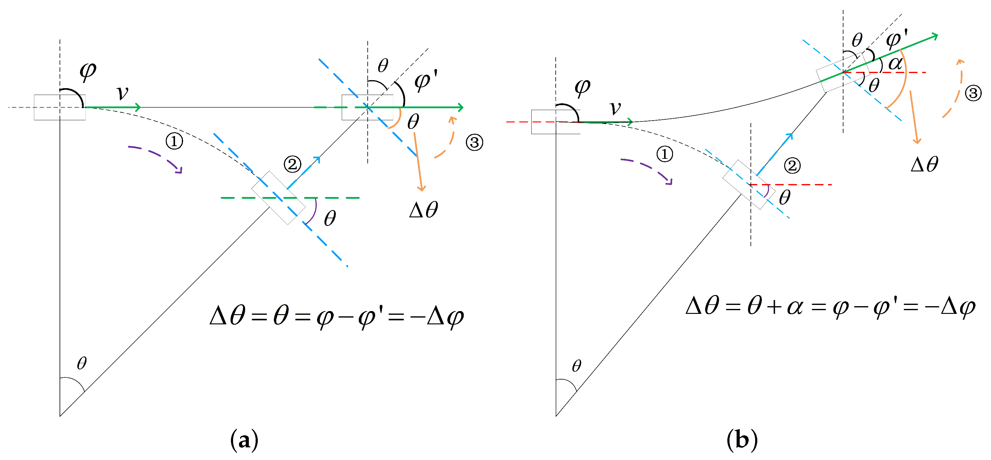
When radar performs two-dimensional ISAR imaging of a target, the radar’s line-of-sight direction and the target’s motion direction form the imaging plane of the radar on the target. With the assumption that the target does not exhibit significant maneuverability in the horizontal direction in a short period of time, the imaging plane remains unchanged during the imaging process. In this case, the target’s motion trajectory can be reflected on the two-dimensional plane. When the target is flying in a straight line, the motion states of the target at moment 0 and moment t are obtained as shown in Figure 1. Numbers ➀ to ➂ represent the three processes after the decomposition of the target movement. $\phi$ and ${\phi }^{\prime }$ are the yaw angles at moment 0 and moment, respectively. t. It can be seen that the effective rotation angle of target $\mathsf{\Delta }\theta$ is equal to the rotation angle of the target moving in a circular motion around radar $\theta$, which is also equal to the change in yaw angle along the radar’s line-of-sight direction $\left|\mathsf{\Delta }\phi \right|=\left|{\phi }^{\prime }-\phi \right|$, that is, $\mathsf{\Delta }\theta =\theta =\left|\mathsf{\Delta }\phi \right|$.

When the target is flying along a curved path, the motion states of the target at moment 0 and moment t are obtained, as shown in Figure 1. The effective rotation angle of the target is $\mathsf{\Delta }\theta =\alpha +\theta$, where $\alpha$ is the deviation of the target’s velocity direction in the geodetic reference system. At the same time, the effective rotation angle of the target is also equal to the change in yaw angle along the radar’s line-of-sight direction, that is, $\mathsf{\Delta }\theta =\alpha +\theta =\left|\mathsf{\Delta }\phi \right|$.

Based on the above analysis, the effective rotation angle of the target is the change in the yaw angle along the radar’s line of sight $\left|\mathsf{\Delta }\phi \right|$. Therefore, by acquiring information on target search and tracking, and by observing changes in the yaw angle along the radar’s line of sight, one can derive the value of the target’s equivalent rotational angular velocity over time by differentiating the yaw angle with respect to time: $\omega \left(t\right)=\mathrm{d}\phi \left(t\right)/\mathrm{d}t$. However, considering that errors may be larger when measuring a single variable, the effective rotation angle is further divided into two parts: one part is the rotation angle of the target moving in a circular motion around radar $\theta$, and another part is the deviation of the target’s velocity direction in the geodetic reference system $\alpha$. Therefore, equivalent rotational angular velocity can also be divided into two parts: ${\omega }_{\theta }\left(t\right)$ and ${\omega }_{\alpha }\left(t\right)$. Based on the relationship between linear velocity and angular velocity in a circular motion, an expression for ${\omega }_{\theta }\left(t\right)$ can be derived as follows:

$${\omega }_{\theta }\left(t\right)=\frac{\left|\mathbf{v}\left(t\right)\right|sin\phi \left(t\right)}{R\left(t\right)},$$

(5)

where $\mathbf{v}\left(t\right)$ is the target’s velocity vector, and $R\left(t\right)$ is the distance between the target and the radar. Expressions for $\alpha \left(t\right)$ and ${\omega }_{\alpha }\left(t\right)$ can be derived as follows:

$$\alpha \left(t\right)=arccos\frac{{\left|\mathbf{v}\left(0\right)\right|}^2+{\left|\mathbf{v}\left(t\right)\right|}^2-{\left|\mathbf{v}\left(t\right)-\mathbf{v}\left(0\right)\right|}^2}{2\left|\mathbf{v}\left(0\right)\right|\left|\mathbf{v}\left(t\right)\right|},$$

(6)

$${\omega }_{\alpha }\left(t\right)=\mathrm{d}\left(\alpha \left(t\right)\right)/\mathrm{d}t,$$

(7)

where $\left|\mathbf{v}\left(0\right)\right|$ is the velocity of the target at the start of the scheduling period. Therefore, the expression for the second type of equivalent rotational angular velocity is as follows:

$$\omega \left(t\right)={\omega }_{\theta }\left(t\right)\pm {\omega }_{\alpha }\left(t\right)=\frac{\left|\mathbf{v}\left(t\right)\right|sin\phi \left(t\right)}{R\left(t\right)}\pm \frac{\mathrm{d}\alpha \left(t\right)}{\mathrm{d}t}.$$

(8)

When the target is yawing in the positive direction of the z-axis of the geodetic coordinate system, a positive sign is chosen. In order to reduce the impact of measurement errors on the final result, the expressions for both types of equivalent rotational angular velocity are integrated to obtain the final expression as follows:

$$\omega \left(t\right)=(\frac{\left|\mathbf{v}\left(t\right)\right|sin\phi \left(t\right)}{R\left(t\right)}\pm \frac{\mathrm{d}\alpha \left(t\right)}{\mathrm{d}t}+\frac{\mathrm{d}\phi \left(t\right)}{\mathrm{d}t})/2.$$

(9)

From Equation (9), it can be seen that the target’s equivalent rotational angular velocity is directly related to the target’s velocity, distance, and yaw angle. When the target’s motion states change, the equivalent rotational angular velocity will inevitably change as well.

Therefore, in combination with the above analysis, considering that the target cannot exhibit significant maneuvering when being imaged with the RD algorithm lest it produce an obvious defocusing phenomenon, this paper selects time periods when the target’s equivalent rotational angular velocity is both large and stable as the optimal observation periods for imaging the target and evaluates the smoothness of these observation periods by analyzing the magnitude of angular acceleration.

2.3. Resource Scheduling Model Construction

To solve the resource scheduling problem in multi-target ISAR imaging tasks, we first need to model the problem. Firstly, the optimal scheduling strategy output by the model consists of two parts: the imaging task duration T and the pulse allocation sequences for each target, where the pulse allocation sequences for each target are stored in the scheduling vector x. The vector is initialized as a zero vector of length 1 $\times N_T$, where $N_T=T·PRF$ is the total number of pulses within the imaging task duration, and each element in the vector represents which target is being observed by the radar using the current pulse. If the kth target is imaged at the ith pulse, then $x\left(i\right)=k$, with the specific expression shown in Equation (10) as follows:

$$x\left(i\right)=\left\{\begin{array}{cc}0,& notused\\ 1,& k=1\\ 2,& k=2\\ \dots & \\ N,& k=N\end{array}\right\},$$

(10)

where N is the total number of targets to be imaged in the detection area.

Our goal is to accomplish the multi-target imaging tasks using as few resources as possible while ensuring the success rate of task scheduling. Therefore, the objective function should include the following points: (1) ensure a certain success rate of task scheduling; (2) ensure that targets with higher priority are allocated resources for imaging first; (3) minimize resource consumption as much as possible.

The first point, the success rate of task scheduling, can be measured by the ratio of the number of successfully scheduled targets to the total number of targets to be imaged. Similarly, for the second point, the ratio of the sum of priority levels of successfully scheduled targets to the sum of priority levels of all targets to be imaged can be used as a measure. Regarding the third point, in one of the working modes of a multi-function phased array radar, a specific time segment is often reserved for imaging tasks. Therefore, the shorter the imaging task duration, the less resource consumption. Additionally, since we allocate sparse pulse sequences to each target, we define a metric called pulse utilization rate to measure resource utilization within the imaging task duration. If the pulse utilization rate is too low, it indicates significant resource waste within the imaging task duration and should be further reduced by shortening the imaging task duration.

Based on the above analysis, the following three performance indicators are defined:

(1)

Success Rate of Task Scheduling (SRTS)

$$SRTS=\frac{n_s}{N},$$

(11)

where $n_s$ is the number of targets successfully scheduled, $n_s={\displaystyle \sum _{k=1}^N}{X}_k$.

(2)

Priority Implementation Rate (PIR)

$$PIR=\frac{{\displaystyle \sum _{k=1}^N}{P}_k{X}_k}{{\displaystyle \sum _{k=1}^N}{P}_k},$$

(12)

where $P_k$ is the priority of the kth target, and $X_k$ can only take the values 1 or 0. $X_k=1$ indicates that the kth target is scheduled, while $X_k=0$ indicates that it is not. Then, $X_k$ can be expressed as:

$$X_k=\left\{\begin{array}{cc}1& {\displaystyle \sum _{i=1}^{N_T}}\frac{i}{\left|i\right|}\left|\left(x\right(i)=k)\right.\ne 0\\ 0& else\end{array}\right..$$

(13)

(3)

Pulse Utilization Rate (PUR)

$$PUR=\frac{M_s}{N_c},$$

(14)

where $M_s$ is the total number of pulses used within the imaging task duration, $M_s={\displaystyle \sum _{k=1}^N}{\displaystyle \sum _{i=1}^{N_T}}\frac{i}{\left|i\right|}\left|\left(x\right(i)=k)\right.$, and $N_c$ is the total number of pulses during the imaging task duration.

Based on the performance indicators set above, with the scheduling vector x and the imaging task duration T as the variables to be optimized, a radar resource scheduling model for multi-target ISAR imaging is constructed:

$$\begin{array}{cc}\hfill & \underset{x,T}{max}\{l_1·\frac{{\displaystyle \sum _{k=1}^N}{P}_k·X_k}{{\displaystyle \sum _{k=1}^N}{P}_k}+l_2·\frac{{\displaystyle \sum _{k=1}^N}{X}_k}{N}+l_3·\frac{{\displaystyle \sum _{k=1}^N}{\displaystyle \sum _{i=1}^{T·PRF}}\frac{i}{\left|i\right|}\left|\left(x\right(i)=k)\right.}{T·PRF}\}\hfill \\ \hfill & \begin{array}{cc}\hfill s.t.& T_a<T<T_b,T\in Z^{+}\hfill \\ \hfill & t_s\le t_k\le t_s+T-T_k\hfill \\ \hfill & \mathsf{\Delta }{\theta }_k={\int }_{t_k}^{t_k+T_k}{\omega }_k\left(t\right)dt,N_k=T_k·PRF\hfill \\ \hfill & max\left({\varpi }_k(t_k:t_k+T_k)\right)<{\varpi }_0\hfill \\ \hfill & M_k=\sum _{i=1}^{N_T}\frac{i}{\left|i\right|}\left|\left(x\right(i)=k)\right.\hfill \\ \hfill & M_k\ge c_1·K_k·ln{N}_k\hfill \\ \hfill & {\displaystyle \sum _{k=1}^N}{M}_k·X_k/\phantom{M_k·X_{k}PRF}PRF\le T\hfill \end{array}.\hfill \end{array}$$

(15)

The objective function is the weighted sum of the three performance indicators; $l_1$, $l_2$, and $l_3$ are, respectively, the weights of these three indicators, and they are respectively set to 0.4, 0.3, and 0.3 here. The first constraint ensures that imaging task duration falls within a predefined range $[T_a,T_b]$. The second constraint indicates that the target’s observation period must be within the imaging task duration, where $t_s$ is the start time of scheduling, and $t_k$ and $T_k$ are, respectively, the start time of observation and coherent accumulation time for the kth target. The third constraint requires sufficient rotation angle $\mathsf{\Delta }{\theta }_k$ during observations to achieve desired azimuth resolution, and $N_k$ is the number of pulses emitted during coherent accumulation time. The fourth constraint represents that the observation period should satisfy the condition of smoothness, where ${\varpi }_k$ is the angular acceleration, which can be obtained by differentiating the equivalent rotational angular velocity with respect to time t, and ${\varpi }_0$ is the threshold of angular acceleration that satisfies the imaging quality requirements. The fifth constraint indicates that the target’s observation dimension can be retrieved through scheduling vector x. The sixth constraint indicates that the observation dimension must satisfy conditions required for reconstructing the original signal using the OMP algorithm. The seventh constraint states that the total number of transmitted pulses during observations cannot surpass available pulses as defined by the imaging task duration.

2.4. Algorithm for Model Solving

Through analysis, it can be determined that Equation (15) presents a multi-dimensional and computationally intensive optimization challenge in resource scheduling, and it is challenging to solve using conventional gradient-based mathematical methods. Therefore, in response to this problem, we have developed a feedback-based closed-loop search optimization method. This method is inspired by the evolutionary algorithm’s approach of continuously generating and refining candidate solutions to find the optimal solution. Feedback is introduced into the candidate solution mutation mechanism, allowing for directed mutation of candidate solutions based on the output of each iteration, ultimately converging on an optimal solution. The solution method consists of two main parts: one part is a specific method for allocating pulse sequences to each target when the imaging task duration is determined, which we call the inner loop allocation method; the other part is the closed-loop search optimization process for the imaging task duration, referred to as the outer loop search method. Next, we will provide a detailed description of the solution method.

2.4.1. Prior Information Acquisition

First, we need to obtain the necessary prior information. The radar first transmits a small number of pulses to the targets to obtain information about the targets’ size, sparsity, and other relevant data. Then, utilizing the target tracking information, the future motion states of the target are predicted, including parameters such as velocity, distance, and yaw angle information. Based on this, the target’s priority, equivalent rotational angular velocity, and optimal observation period can be calculated.

(1)

Calculate the target’s azimuth resolution and coherent accumulation angle.

Using the method described in Reference [14], the target’s azimuth size $S_{kx}$ and sparsity $K_k$ are estimated based on the coarse ISAR image obtained from transmitting a small number of pulses. Then, assuming a reference size $S_{x\_ref}$ and a reference azimuth resolution ${\rho }_{ref}$, the azimuth resolution of the target can be obtained based on the target’s size as follows:

$${\rho }_k=\frac{S_{kx}}{S_{x\_ref}}{\rho }_{ref}.$$

(16)

Then, based on the expression for azimuth resolution, the expression for the coherent accumulation angle can be obtained as follows:

$$\mathsf{\Delta }{\theta }_k=\frac{\lambda }{2{\rho }_k}.$$

(17)

(2)

Calculate the priority of the target.

Typically, we consider targets with high flight velocity, close proximity to the radar, and movement towards the radar to pose a greater threat and therefore require a higher priority. Thus, when calculating the priority of a target, we focus on three factors: the target’s flight velocity ${\mathbf{v}}_k\left(t\right)$, the distance from the target to the radar $R_k\left(t\right)$, and the yaw angle ${\phi }_k\left(t\right)$. Taking into account fluctuations in the target’s motion state, the priority is set as follows:

$$P_k={\omega }_1\frac{{R_k}^{\prime }}{max\left({R_k}^{\prime }\right)}+{\omega }_2\frac{{{\mathbf{v}}_k}^{\prime }}{max\left({{\mathbf{v}}_k}^{\prime }\right)}+{\omega }_3\frac{{{\phi }_k}^{\prime }}{max\left(\left|{{\phi }_k}^{\prime }\right|\right)},$$

(18)

where ${R_k}^{\prime }=1/min\left(R_k\left(t\right)\right)$, ${{\mathbf{v}}_k}^{\prime }=max\left(\left|{\mathbf{v}}_k\left(t\right)\right|\right)$, and ${{\phi }_k}^{\prime }=-cos\left({\phi }_k\left(0\right)\right)$. ${R_k}^{\prime }$ is the reciprocal of the shortest distance from target k to the radar within the imaging task duration, representing the threat level due to proximity; ${{\mathbf{v}}_k}^{\prime }$ is the maximum velocity of target k within the imaging task duration; and ${{\phi }_k}^{\prime }$ is the negative cosine value of the initial yaw angle of target k, used to characterize the threat level of the target’s flight direction. ${\omega }_1$, ${\omega }_2$, and ${\omega }_3$ are, respectively, the weights of these three factors, and weights can be set for different scenarios according to their requirements.

(3)

Calculate the optimal observation period for the target.

First, based on the predicted data of the target’s motion velocity, distance, and yaw angle over time within the imaging task duration, the data of the target’s equivalent rotational angular velocity over time ${\omega }_k\left(t\right)$ can be calculated via Equation (9). Then, the angular acceleration ${\varpi }_k\left(t\right)$ can be obtained by differentiating the equivalent rotational angular velocity with respect to time t, which is used to evaluate the smoothness of the angular velocity.

The optimal observation period for each target can be determined by solving the following optimization model:

$$\begin{array}{cc}\hfill & min{T}_c\hfill \\ & \begin{array}{cc}s.t.\hfill & {\int }_{t_0}^{t_0+T_c}{\omega }_k\left(t\right)dt=\mathsf{\Delta }{\theta }_k\hfill \\ \hfill & 0\le t_0\le T-T_c\hfill \\ \hfill & 0<T_c<T\hfill \\ \hfill & {\varpi }_k=d\left({\omega }_k\left(t\right)\right)/dt\hfill \\ \hfill & max\left({\varpi }_k(t_0:t_0+T_c)\right)<{\varpi }_0\hfill \end{array},\hfill \end{array}$$

(19)

where $t_0$ and $T_c$ are the variables to be optimized in the model, $\left[t_0,t_0+T_c\right]$ represents the optimal observation period being sought, T is the imaging task duration, and ${\varpi }_0$ is the threshold of angular acceleration that satisfies the imaging quality requirements, representing the requirement for smoothness of angular acceleration within the optimal observation period. The solution to this model can be obtained through a single mathematical traversal.

2.4.2. Inner Loop Allocation Method

When the imaging task duration is determined, the radar imaging resource optimization scheduling problem mainly aims to maximize the SRTS and PIR and to allocate pulse sequences to each target within the imaging task duration. The mathematical model serves as a simplification of the model constructed in this paper and can be expressed as follows:

$$\begin{array}{cc}\hfill & \underset{x}{max}\{0.5·\frac{{\displaystyle \sum _{k=1}^N}{P}_k·X_k}{{\displaystyle \sum _{k=1}^N}{P}_k}+0.5·\frac{{\displaystyle \sum _{k=1}^N}{X}_k}{N}\}\hfill \\ \hfill & \begin{array}{cc}s.t.\hfill & t_s\le t_k\le t_s+T-T_k\hfill \\ \hfill & \mathsf{\Delta }{\theta }_k={\int }_{t_k}^{t_k+T_k}{\omega }_k\left(t\right)dt,N_k=T_k·PRF\hfill \\ \hfill & max\left({\varpi }_k(t_k:t_k+T_k)\right)<{\varpi }_0\hfill \\ \hfill & M_k={\displaystyle \sum _{i=1}^{N_T}}\frac{i}{\left|i\right|}\left|\left(x\right(i)=k)\right.\hfill \\ \hfill & M_k\ge c_1·K_k·ln{N}_k\hfill \\ \hfill & {\displaystyle \sum _{k=1}^N}{M}_k·X_k/\phantom{M_k·X_{k}PRF}PRF\le T\hfill \end{array}.\hfill \end{array}$$

(20)

For the solution to Equation (20), an inner loop allocation method is proposed. Due to the fact that radar imaging targets are often threatening, it is necessary to prioritize allocating resources for imaging to high-priority (i.e., high threat level) targets. Therefore, the main idea of the method is to allocate pulses to each target individually based on priority and on the optimal observation period for each target. To ensure that the pulses allocated to each target meet the sparse reconstruction condition and achieve a better imaging quality, the pulse sequence allocated to the target should satisfy conditions such as continuous observation during the observation period, a sufficient number of pulses, and relatively even distribution of sparse pulses. To achieve the realization of the third condition, we divide the observation period into several small segments and then allocate a certain number of pulses to the target in each segment. For example, if a total of M pulses needs to be allocated, and we divide the observation pulses into n segments, then $M/n$ pulses need to be allocated to the target in each segment. By employing this method, we ensure a certain degree of uniform distribution of pulse sequences within the observation period.

The specific steps of the inner loop allocation method are as follows:

Step 1: Perceive the characteristics of the target and predict the target’s motion state;

Step 2: Evaluate the priority of the targets;

Step 3: Calculate the optimal observation period for each target within the imaging task duration;

Step 4: Sort targets according to priority and allocate observation pulses to each target sequentially. When allocating, prioritize giving each target its optimal observation period. If resources are insufficient within this optimal period, then, based on experience, search for an available suboptimal observation period near it. The allocated pulses must comply with sparse reconstruction conditions;

Step 5: When all targets have been assigned or when resources are insufficient, the allocation process ends, and the pulse allocation sequence for each target can be obtained.

2.4.3. Outer Loop Search Method

For the outer loop search method, we introduce a feedback structure based on evolutionary algorithms, which quickly converges to the optimal solution of the problem after a limited number of iterations, obtaining the optimal imaging task duration.

Firstly, an evaluation indicator called Degree of Excellence (DoE) is defined according to the objective function in the model, as shown in Equation (21) as follows:

$$DoE=\frac{SRTS-S_0}{\left|SRTS-S_0\right|}·(l_1·PIR+l_2·SRTS+l_3·PUR),$$

(21)

where $\frac{SRTS-S_0}{\left|SRTS-S_0\right|}$ represents the positive or negative nature of the DoE. Only when SRTS meets certain requirements can DoE be positive, and $l_1$, $l_2$, and $l_3$ are respectively set to 0.4, 0.3, and 0.3.

Then, we design the feedback structure as shown in Figure 2.

The mutation operator in the figure is defined as follows:

$$muor=\lfloor 10\times (PUR-SRTS)\rfloor ,$$

(22)

$$operator=\left\{\begin{array}{c}\begin{array}{cc}1,& muor\le 0\&DoE\le 0\end{array}\hfill \\ \begin{array}{cc}-1,& muor\le -T\&DoE>0\end{array}\hfill \\ \begin{array}{cc}\mathbf{break},& muor=0\&DoE>0\end{array}\hfill \\ \begin{array}{cc}muor,& else\end{array}\hfill \end{array}\right.,$$

(23)

where $muor$ is a coarse operator that is designed based on experience, and it is feasible in most cases. For example, in the case where DoE is a positive value, when SRTS is high but PUR is low, it indicates that the imaging task duration has become too long, and the imaging task duration should be mutated towards shortening. At this point, $muor$ takes a negative value. Since we usually set the imaging task duration as an integer, the operators here are also set as integers. Compared to setting the operator as a decimal, setting it as an integer can significantly reduce the number of iterations, thereby reducing the computational complexity of the algorithm. The adjustment step size of the mutation operator is set to 1; a more detailed definition for the operator is shown in Equation (23). When $muor$ is calculated not as a positive value and DoE is also not positive, the obtained solution does not meet the condition of SRTS, and the imaging task duration should not be further shortened. Therefore, in this case, the operator is set to 1 for calibration. When $muor$ is calculated as less than $-T$ and DoE is a positive value, it indicates that the mutation operator value is too large. In order to avoid a negative value for the imaging task duration, the operator is set to −1 for calibration. When $muor$ is calculated as equal to 0 and DoE is a positive value, it indicates that both PUR and SRTS have reached a high level. The obtained solution at this point is satisfactory, and the iterative process can be terminated.

The main idea of the outer loop search method is as follows: initially, based on empirical values, an initial solution is determined, which includes an imaging task duration and its corresponding pulse allocation sequence for each target. Then, we calculate the SRTS, PIR, and PUR, and the DoE of the current solution can also be obtained. Following this, a mutation operator is constructed as feedback based on SRTS and PUR, which is utilized to mutate the imaging task duration. After mutation, a new imaging task duration can be obtained, and then the algorithm proceeds to the next iteration. After a limited number of iterations, if T starts to oscillate slightly in a regular pattern and DoE no longer increases, we consider that T has converged. At this point, the mutation stops, and the scheduling strategy with the highest DoE is selected as the optimal scheduling strategy, which includes an imaging task duration and its corresponding pulse allocation sequence for each target.

Finally, the adaptive radar resources scheduling algorithm for multi-target ISAR imaging based on optimal observation periods is described in Algorithm 1.

Algorithm 1 Adaptive Radar Resource Scheduling Algorithm for Multi-Target Imaging Based on Optimal Observation Periods

Input: N, $S_k$, $K_k$, ${\mathbf{v}}_k\left(t\right)$, $R_k\left(t\right)$, ${\phi }_k\left(t\right)$, and $T_0$; Output: $x_{best}$ and $T_{best}$;   1: Calculate the equivalent rotational angular velocity ${\omega }_k\left(t\right)$ and angular acceleration ${\varpi }_k\left(t\right)$ according to the input;   2: Calculate the target’s azimuth resolution ${\rho }_k$ via (16), the coherent accumulation angle $\mathsf{\Delta }{\theta }_k$ via (17), and the priority $P_k$ via (18);   3: Initialize $maxDoE=0$, $T=T_0$;   4: Sort the targets in order of priority to get the sorted order I;   5: while ¬(T has converged) do   6:    Initialize $x=[0,0,\dots ,0]$;   7:    for i=1:N do   8:        $k=I\left(i\right)$;   9:        Calculate the optimal observation period for the target by solving the optimization model of Equation (19);   10:      Calculate the observation dimension $M_k=c_1·K_k·ln{N}_k$, the observation period $x_k=x(\frac{t_k}{PRF}:\frac{t_k+T}{PRF})$, and the free pulse in $x_k$: $free\_pulse=find(x_k=0)$;   11:      if $count(free\_pulse)\ge M_k$ then   12:         Select $M_k$ pulse in $free\_pulse$ as $K_{pulse}$, make $x\left(K_{pulse}\right)=k$;   13:         Update x;   14:      else   15:         Find another available period around the optimal period;   16:         Update x;   17:         if no available period exit then   18:           Break;   19:         end if   20:      end if   21:    end for   22:    Get the $PIR$, $SRTS$, $PUR$ and calculate the $DoE$, $operator$;   23:    if $DoE>maxDoE$ then   24:      $maxDoE=DoE$;   25:      $T_{best}=T$;   26:      $x_{best}=x$;   27:    end if   28:    $T=T+operator$;   29: end while   30: return $T_{best}$, $x_{best}$

3. Simulations

3.1. Algorithm Effectiveness Verification

Assuming the radar emits a linear frequency modulated signal, the carrier frequency of the emitted signal $f_c=10$ GHz, the bandwidth $B=300$ MHz, the range resolution ${\rho }_r=0.5$ m, the pulse repetition frequency $PRF=1000$ Hz, the pulse width $T_p=1$ µs, the baseline size of the target in azimuth $S_{x\_ref}=25$ m, the required azimuth resolution ${\rho }_{ref}=0.5$ m, the threshold for SRTS $S_0=0.99$, the angular acceleration threshold is set to ${\varpi }_0=2\times {10}^{-4}$ through several simulation experiments, and ${\omega }_1$, ${\omega }_2$, and ${\omega }_3$ are respectively set to 0.3, 0.3, and 0.4 according to the expert experience.

Assuming there are a total of 20 targets to be imaged within the radar detection area, the target parameters are shown in

Table 1. Target parameters.

	Size (m)	Sparsity		Size (m)	Sparsity
Target 1	21.45	40	Target 11	25.5	45
Target 2	41.87	87	Target 12	21	46
Target 3	22.5	47	Target 13	26	40
Target 4	65.5	134	Target 14	28.5	52
Target 5	23	50	Target 15	30	62
Target 6	23.5	48	Target 16	21.5	43
Target 7	24	42	Target 17	24	42
Target 8	23	45	Target 18	18.5	41
Target 9	66	146	Target 19	19	39
Target 10	17	36	Target 20	28	54

. Among them, size and sparsity represent the size and sparsity of the targets in the azimuth direction. Figure 3 shows the scattering point models of two of these targets (Target 4 and Target 8). Each target is approximately 50 km away from the radar and moves at a uniform or variable speed at different angles within the radar detection area. The angular velocity of each target over time is shown in Figure 4.

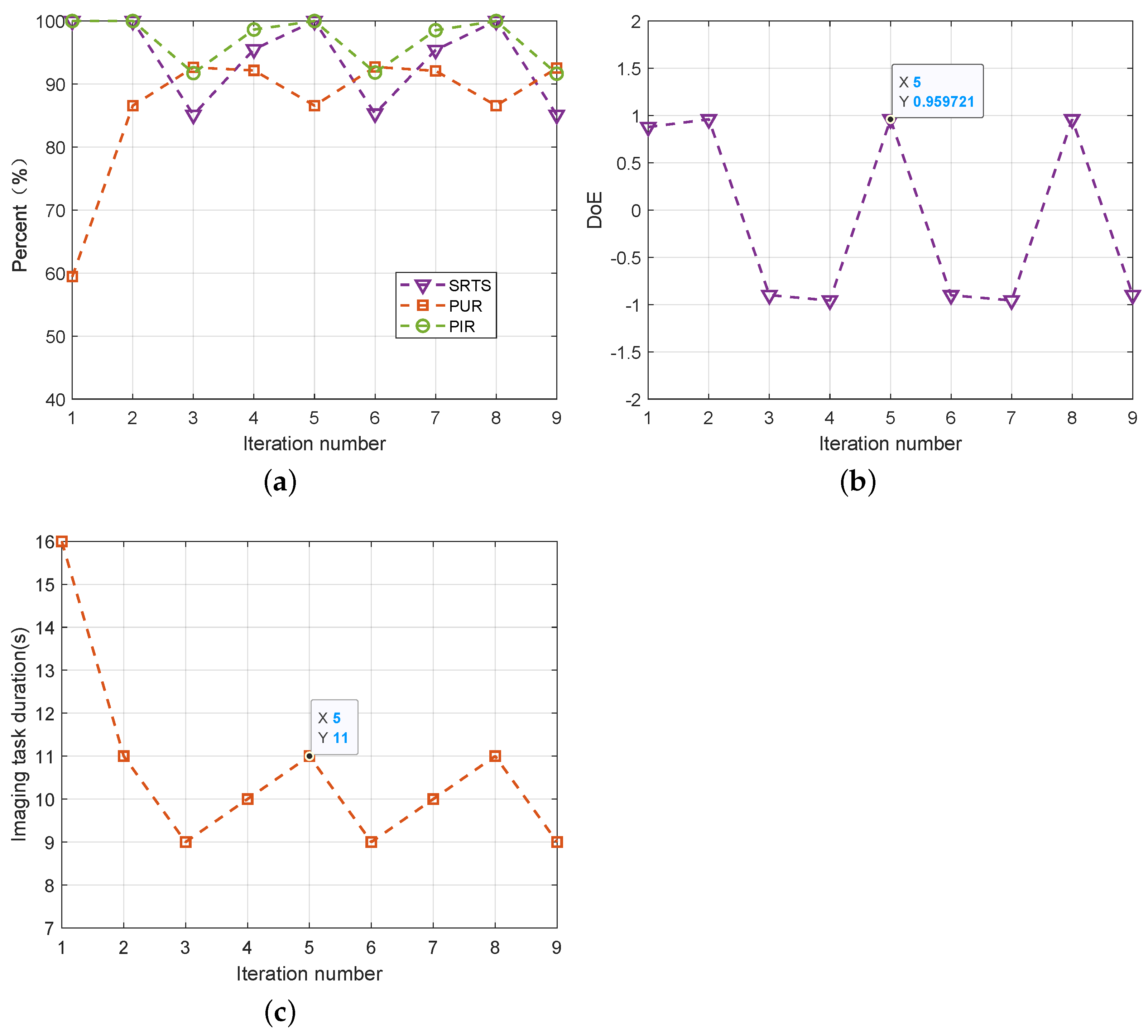
Using the algorithm proposed in this paper, an optimal scheduling strategy for radar imaging of 20 targets can be achieved after a finite number of iterations. To avoid randomness, 100 Monte Carlo experiments were conducted for the inner loop allocation method in each iteration, and the changes in three performance indicators with the number of iterations are shown in Figure 5a. Furthermore, the graphs of DoE and imaging task duration varying with the number of iterations are calculated and shown in Figure 5b,c.

From Figure 5, it can be observed that the parameters in all three subplots start oscillating after the 3rd iteration, and the solution with the highest DoE will be selected as the optimal scheduling strategy. From Figure 5b, it can be seen that the solution obtained in the 5th iteration has the highest DoE, and from the corresponding position in Figure 5c, the imaging task duration is 11 s. Therefore, we can conclude that, for the scenario with 20 targets in this experiment, an imaging task duration of 11 s can maximize the overall system efficiency. Thus, an imaging task duration of 11 s and its corresponding pulse allocation sequence for each target constitute the optimal scheduling strategy.

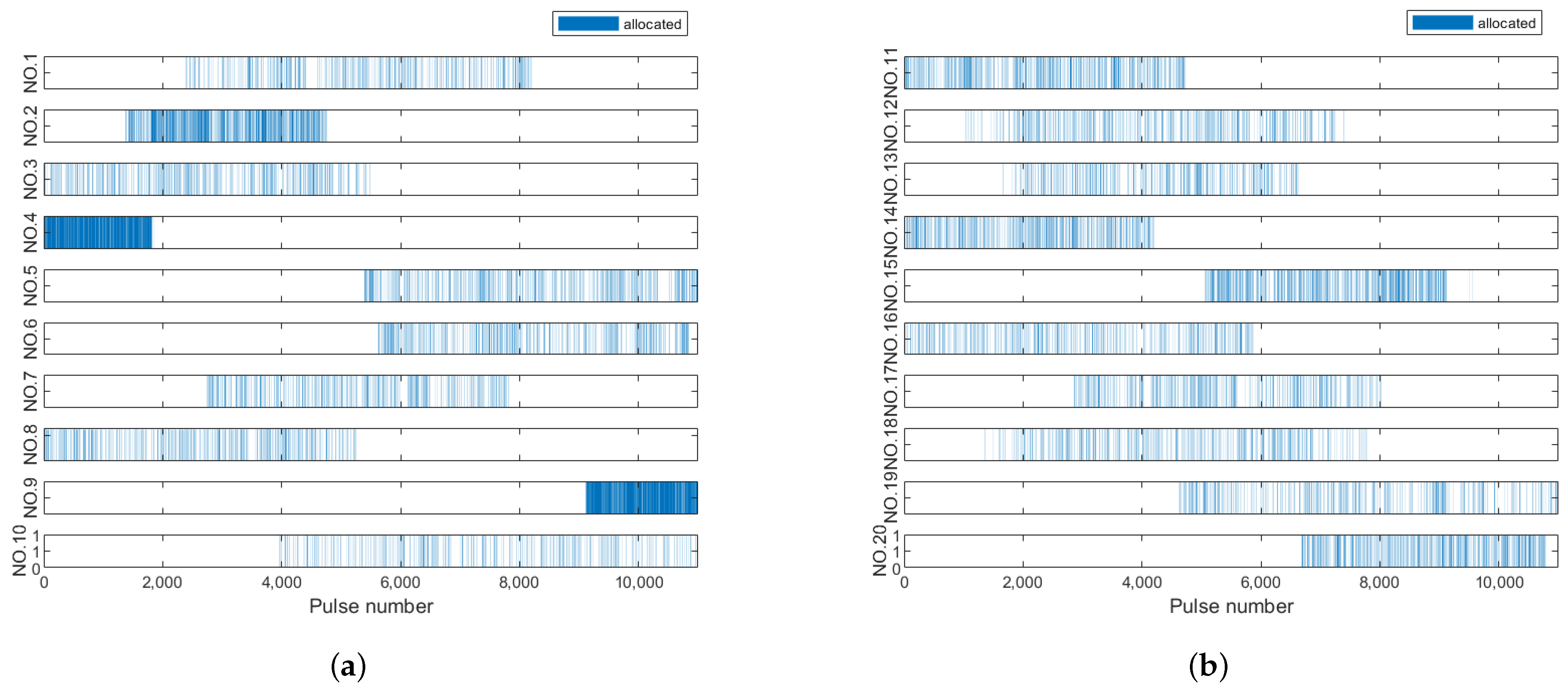
At the same time, the experimental results provide the pulse allocation sequence for each target when the imaging task duration is set to 11 s, as shown in Figure 6. When PRF is set to 1000 Hz, 11 s means emitting 11,000 pulses. Each subplot in Figure 6 represents the sequence of observation pulses assigned to each target by the radar, and the assigned pulses are indicated by blue lines.

From Figure 6, it can be observed that the proposed algorithm successfully assigns observation pulses to all of the targets, achieving an SRTS of 100% and a PIR of 100%; the PUR is determined as 86.57% by calculation. For Target 7, which has the highest priority, its optimal observation period of [2744, 7821] is allocated first. However, due to limited resources, Target 1, which has the lowest priority, does not receive its optimal observation period of [1, 5817]. Instead, the period [2372, 8178] is allocated. For Target 4 and Target 9, which are large in size and have a greater number of scattering points, the required coherent accumulation time is shorter due to their higher resolution. However, due to their greater sparsity, a larger number of observation pulses is needed. Although the coherent accumulation time for other targets is slightly longer, their sparsity is lower, and the distribution of observation pulses is more dispersed.

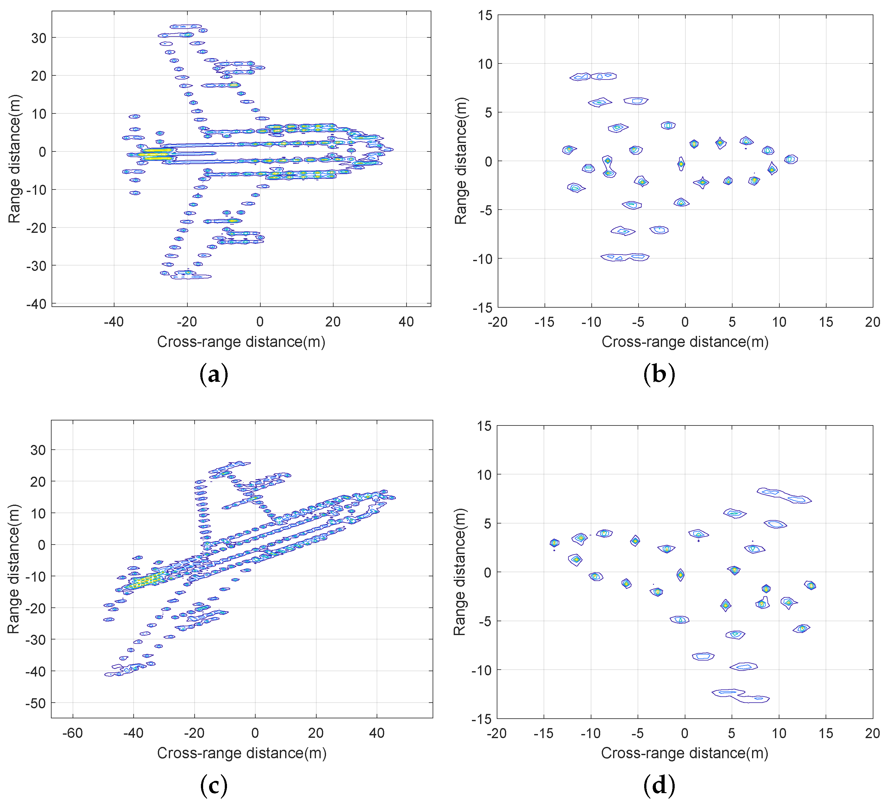
Finally, based on the scheduling results, the targets are observed and imaged using the sparse-aperture ISAR imaging algorithm, with the results of some typical targets shown in Figure 7. Lines of different colors in the figure represent different magnitudes of scattering coefficients. The imaging results of Target 4, Target 8, Target 9, and Target 17 are displayed. As can be seen from Figure 7, the shapes and structures of the targets in the imaging results are clear and consistent with their true scattering distributions.

The image contrast of the imaging result for each target is shown in

Table 2. The image contrast of the imaging result for each target.

Image Contrast
Target 1	18.7298	Target 6	16.7991	Target 11	15.43178	Target 16	17.7603
Target 2	17.2339	Target 7	16.7066	Target 12	18.8842	Target 17	16.4868
Target 3	17.4812	Target 8	17.5831	Target 13	18.5087	Target 18	19.2912
Target 4	7.7819	Target 9	7.2393	Target 14	15.2905	Target 19	16.7248
Target 5	17.7054	Target 10	18.779	Target 15	15.4148	Target 20	12.2694

. Image contrast is the normalized standard deviation of the image. The greater the image contrast, the higher the focus of the image and the better the image quality.

The experiment proves that the proposed algorithm achieves a rational allocation of radar resources among various targets. At the same time, according to the data in Table 2, it can be demonstrated that the imaging results obtained by observing the targets based on the scheduling results are satisfactory in terms of quality.

3.2. Comparative Performance Analysis

In order to verify the performance advantages of the algorithm proposed in this paper, it is compared with the existing algorithms. The main idea of the existing resource optimization scheduling algorithm for multi-target imaging based on single-base radar [14] is to allocate a limited number of observation pulses to each target according to target feature cognition, and then target imaging can be achieved based on sparse-aperture ISAR imaging algorithm. Specifically, it first evaluates the priority or scheduling benefit of each target based on the target detection and identification outcomes. Then, according to the priority or scheduling benefit, it randomly assigns a limited number of observation pulses to each target sequentially without considering the impact of optimal observation periods on the resource scheduling strategy. Finally, the target imaging can be achieved by using the sparse-aperture ISAR imaging algorithm according to the scheduling results (hereinafter referred to as Algorithm 2).

Furthermore, in order to validate the necessity of including an angular velocity smoothness constraint and performing imaging task duration optimization in the algorithm proposed in this paper, we consider using only the maximum angular velocity as the sole criterion for optimal observation period selection to illustrate its impact and make it a comparative algorithm (hereinafter referred to as Algorithm 3).

Since Algorithms 2 and 3 do not take into account the optimization of the imaging task duration, the imaging task duration is firstly fixed at 10 s. The scheduling performance of the three algorithms is shown in

Table 3. Scheduling performance of the three algorithms.

	SRTS	PIR	PUR
Algorithm 1	0.955	0.986431	0.921626
Algorithm 2	0.869	0.896871	0.834812
Algorithm 3	0.99	0.993156	0.921178

.

From Table 3, it can be seen that all the performance indicators of the proposed algorithm are significantly better than Algorithm 2 and, compared with Algorithm 3, the performance is comparable.

Taking Target 8 as an example, the scheduling and imaging results of the three algorithms are shown in Figure 8. To facilitate the observation of the relationship between the pulse allocation method and the equivalent rotation angular velocity, we have displayed the pulse allocation sequence in the angular velocity–time diagram of Target 8, as shown in Figure 8a,c,e.

From Figure 8, it can be observed that the proposed algorithm, which considers angular velocity smoothness constraints, selects a slightly lower but relatively stable angular velocity time period as the optimal observation period during scheduling, resulting in a higher quality image with an image contrast of 17.5831. Algorithm 2 schedules based on priority from front to back. Given that Target 8 has a higher priority, it selects an earlier time period for observation, also yielding good image quality, with an image contrast value of 17.5397. Algorithm 3, on the other hand, does not account for the smoothness of target motion and selects observation time periods solely based on higher angular velocity. Consequently, this approach leads to images with noticeable defocusing and a significantly lower image contrast of only 15.6305 compared to the first two algorithms.

Therefore, although Algorithm 3 appears to have performance indicators comparable to the algorithm proposed in this paper, its imaging quality is not guaranteed.

In addition, the scheduling performance of the three algorithms was compared under varying numbers of targets. The algorithm proposed in this paper can achieve joint optimization of imaging task duration and the pulse allocation sequence for each target, while Algorithms 2 and 3 require a fixed imaging task duration, which is set to 10 s. The imaging task duration optimization result of the proposed algorithm is shown in Figure 9, and the comparison of performance indicators between different algorithms is shown in Figure 10.

From Figure 9 and Figure 10, it can be seen that the proposed algorithm can adaptively adjust the length of the imaging task duration according to the number of targets, ensuring that both the PUR and SRTS remain at a high level. As the number of targets increases, the rate of growth in imaging task duration accelerates in order to ensure that the pulse sequence meets the sparse reconstruction condition. Additionally, the graph shows that, before reaching 20 targets, while achieving the same or higher SRTS as the other two algorithms, the proposed algorithm can obtain a higher PUR. After exceeding 20 targets, although there is a decline in PUR for the proposed algorithm, it still demonstrates a clear advantage over the other two algorithms in two important aspects: priority implementation rate (PIR) and success rate of task scheduling (SRTS).

Therefore, based on the comprehensive performance comparison analysis above, it can be proven that the algorithm proposed in this paper has an overall performance advantage.

4. Conclusions

In this paper, we addressed the problem of radar resource allocation in multi-target imaging scenarios. Initially, we defined the optimal observation periods of the targets under varying motion states. Subsequently, an adaptive radar resource scheduling algorithm for multi-target ISAR imaging based on optimal observation periods was proposed. This algorithm considers the imaging task duration and the pulse allocation sequence for each target as optimization variables and involves the construction of the radar resource scheduling model for multi-target ISAR imaging. Then, a feedback-based closed-loop search optimization method was proposed to solve this model, ultimately achieving a rational allocation of radar resources among the targets and an enhancement in the overall performance of the radar system.

The collaborative work mechanism and integration of resources among multiple radars in a radar network can enhance its capability beyond that of individual radars, rendering it more suitable for ISAR imaging missions involving aerial and space targets in modern warfare scenarios. Hence, our future research will focus on developing a resource scheduling method for a radar network tailored to 2D and 3D imaging tasks involving multiple targets to improve the efficiency of radar systems.

References

- Bai, X.; Zhang, Y.; Liu, S. High-Resolution Radar Imaging of Off-Grid Maneuvering Targets Based on Parametric Sparse Bayesian Learning. IEEE Trans. Geosci. Remote Sens. 2022, 60, 5112611. [Google Scholar] [CrossRef]
- Tian, X.; Bai, X.; Xue, R.; Qin, R.; Zhou, F. Fusion Recognition of Space Targets with Micro-Motion. IEEE Trans. Aerosp. Electron. Syst. 2022, 58, 3116–3125. [Google Scholar] [CrossRef]
- Wang, Y.; Zhang, Y.; Bai, X. High-Resolution ISAR Imaging With SSFCS Based on Nonparametric Bayesian Learning and Genetic Algorith. IEEE Trans. Geosci. Remote Sens. 2023, 61, 5106612. [Google Scholar] [CrossRef]
- Hovanessian, S.A. Introduction to Synthetic Array and Imaging Radars; Artech House Publishers: Dedham, MA, USA, 1980. [Google Scholar]
- Ausherman, D.A.; Kozma, A.; Walker, J.L.; Jones, H.M.; Poggio, E.C. Developments in Radar Imaging. IEEE Trans. Aerosp. Electron. Syst. 1984, AES-20, 363–400. [Google Scholar] [CrossRef]
- Shi, C.; Tang, Z.; Ding, L.; Yan, J. Multi-Domain Resource Allocation for Asynchronous Target Tracking in Heterogeneous Multiple Radar Networks with Non-Ideal Detection. IEEE Trans. Aerosp. Electron. Syst. 2023, 60, 2016–2033. [Google Scholar] [CrossRef]
- Shi, C.; Wang, Y.; Salous, S.; Zhou, J.; Yan, J. Joint Transmit Resource Management and Waveform Selection Strategy for Target Tracking in Distributed Phased Array Radar Network. IEEE Trans. Aerosp. Electron. Syst. 2022, 58, 2762–2778. [Google Scholar] [CrossRef]
- Yan, J.; Jiao, H.; Pu, W.; Shi, C.; Dai, J.; Liu, H. Radar sensor network resource allocation for fused target tracking: A brief review. Inf. Fusion 2022, 86–87, 104–115. [Google Scholar] [CrossRef]
- Yan, J.; Pu, W.; Zhou, S.; Liu, H.; Greco, M.S. Optimal Resource Allocation for Asynchronous Multiple Targets Tracking in Heterogeneous Radar Networks. IEEE Trans. Signal Process. 2022, 68, 4055–4068. [Google Scholar] [CrossRef]
- Yan, J.; Pu, W.; Zhou, S.; Liu, H.; Bao, Z. Collaborative detection and power allocation framework for target tracking in multiple radar system. Inf. Fusion 2020, 55, 173–183. [Google Scholar] [CrossRef]
- Li, A.; Liao, K.; Ouyang, S. ISAR imaging resource-scheduling algorithm in network radar based on information fusion. J. Eng. 2019, 20, 7078–7082. [Google Scholar] [CrossRef]
- Xu, F.; Wang, R.; Mao, D.; Zhang, Y.; Zhang, Y.; Huang, Y.; Yang, J. Resource Allocation Optimization of Distributed Radar Imaging System Based on Spatial Spectrum Analysis. In Proceedings of the IGARSS 2019—2019 IEEE International Geoscience and Remote Sensing Symposium, Yokohama, Japan, 28 July–2 August 2019; pp. 9101–9104. [Google Scholar] [CrossRef]
- Shao, S.; Zhang, L.; Liu, H. An optimal imaging time interval selection technique for marine targets ISAR imaging based on sea dynamic prior information. IEEE Sens. J. 2019, 19, 4940–4953. [Google Scholar] [CrossRef]
- Chen, Y.; Zhang, Q.; Yuan, N.; Luo, Y.; Lou, H. An adaptive ISAR-imaging-considered task scheduling algorithm for multi-function phased array radars. IEEE Trans. Signal Process. 2019, 63, 5096–5110. [Google Scholar] [CrossRef]
- Meng, D.; Xu, H.; Zhang, Q.; Chen, Y.J. Adaptive scheduling algorithm for ISAR imaging radar based on pulse interleaving. In Machine Learning and Intelligent Communications; Springer: Berlin/Heidelberg, Germany, 2017; pp. 169–178. [Google Scholar] [CrossRef]
- Wang, H.; Liao, K.; Ouyang, S.; Wang, H.; Yang, L. Resource scheduling algorithm optimization for multitarget inverse synthetic aperture radar imaging in radar network. J. Appl. Remote 2021, 15, 016521. [Google Scholar] [CrossRef]
- Du, Y.; Liao, K.F.; Ouyang, S.; Li, J.J.; Huang, G.J. Time and Aperture Resource Allocation Strategy for Multitarget ISAR Imaging in a Radar Network. IEEE Sens. J. 2020, 20, 3196–3206. [Google Scholar] [CrossRef]
- Chen, Y.J.; Zhang, Q.; Luo, Y.; Li, K.M. Multi-Target Radar Imaging Based on Phased-MIMO Technique—Part II: Adaptive Resource Allocation. IEEE Sens. J. 2017, 17, 6198–6209. [Google Scholar] [CrossRef]
- Hu, T.; Liao, K.; Ouyang, S.; Wang, H. Resource Scheduling for Multitarget Imaging in a Distributed Netted Radar System Based on Maximum Scheduling Benefits. Sensors 2022, 22, 6400. [Google Scholar] [CrossRef] [PubMed]
- Wang, D.; Li, K.M.; Zhang, Q.; Lu, X.F.; Luo, Y. A cooperative task allocation game for multi-target imaging in radar networks. IEEE Sens. J. 2021, 21, 7541–7550. [Google Scholar] [CrossRef]
- Chen, V.; Qian, S. Joint time-frequency transform for radar range-Doppler imaging. IEEE Trans. Aerosp. Electron. Syst. 1998, 34, 486–499. [Google Scholar] [CrossRef]
- Stankovic, L.; Thayaparan, T.; Dakovic, M.; Popovic-Bugarin, V. Micro-Doppler removal in the radar imaging analysis. IEEE Trans. Aerosp. Electron. Syst. 2013, 49, 1234–1250. [Google Scholar] [CrossRef]
- Wang, Y.; Chen, X. 3-D Interferometric Inverse Synthetic Aperture Radar Imaging of Ship Target With Complex Motion. IEEE Trans. Geosci. Remote Sens. 2018, 56, 3693–3708. [Google Scholar] [CrossRef]
- Xu, G.; Xing, M.; Xia, X.G.; Zhang, L.; Chen, Q.; Bao, Z. 3D Geometry and Motion Estimations of Maneuvering Targets for Interferometric ISAR With Sparse Aperture. IEEE Trans. Image Process. 2016, 25, 2005–2020. [Google Scholar] [CrossRef] [PubMed]
- Wang, J.; Wu, Y.; Deng, X.; Zhang, L.; Wang, J.; Zhou, L. Highly Maneuvering Target Detection Based on Neural Network and Generalized Radon-Fourier Transform. IEEE Geosci. Remote Sens. Lett. 2023, 20, 3507805. [Google Scholar] [CrossRef]
- Zhang, L.; Xing, M.; Qiu, C.W.; Li, J.; Bao, Z. Achieving Higher Resolution ISAR Imaging With Limited Pulses via Compressed Sampling. IEEE Geosci. Remote Sens. Lett. 2009, 6, 567–571. [Google Scholar] [CrossRef]
- Xu, G.; Zhang, B.; Chen, J.; Hong, W. Structured Low-Rank and Sparse Method for ISAR Imaging With 2-D Compressive Sampling. IEEE Trans. Geosci. Remote Sens. 2022, 60, 5239014. [Google Scholar] [CrossRef]
- Xu, G.; Zhang, B.; Chen, J.; Wu, F.; Sheng, J.; Hong, W. Sparse Inverse Synthetic Aperture Radar Imaging Using Structured Low-Rank Method. IEEE Trans. Geosci. Remote Sens. 2022, 60, 5213712. [Google Scholar] [CrossRef]
- Luo, Y.; Zhang, Q.; Hong, W.; Wu, Y. Waveform design and high-resolution imaging of cognitive radar based on compressive sensing. Sci. China Inf. Sci. 2012, 55, 2590–2603. [Google Scholar] [CrossRef]
- Cheng, P.; Wang, X.; Zhao, J.; Cheng, J. A Fast and Accurate Compressed Sensing Reconstruction Algorithm for ISAR Imaging. IEEE Access 2019, 7, 157019–157026. [Google Scholar] [CrossRef]
Figure 1.
Derivation diagram of the target’s equivalent rotation angle. (a) Target flying in a straight line. (b) Target flying along a curved path.
Figure 2.
Feedback structure.
Figure 3.
Scattering point models. (a) Target 4. (b) Target 8.
Figure 4.
Angular velocity of 20 target over time.
Figure 5.
Indicators varying with iteration number. (a) Three performance indicators varying with iteration number. (b) Degree of Excellence (DoE) varying with iteration number. (c) Imaging task duration varying with iteration number.
Figure 6.
Pulse allocation sequences for 20 targets when the imaging task duration is set to 11 s. (The blue line indicates that the pulse at the current position is assigned to observe the corresponding target). (a) The first 10 targets. (b) The last 10 targets.
Figure 7.
Imaging results. (a) Target 4. (b) Target 8. (c) Target 9. (d) Target 17.
Figure 8.
The scheduling and imaging results of the three algorithms. (The red lines represent the pulses assigned to Target 8 for observation, and they are sparsely distributed.) (a) The scheduling result of the proposed algorithm for Target 8. (b) The imaging result of the proposed algorithm for Target 8. (c) The scheduling result of Algorithm 2 for Target 8. (d) The imaging result of Algorithm 2 for Target 8. (e) The scheduling result of Algorithm 3 for Target 8. (f) The imaging result of Algorithm 3 for Target 8.
Figure 9.
Imaging task duration varying with the number of targets for the proposed algorithm.
Figure 10.
Comparison of performance indicators between different algorithms. (a) PIR varying with the number of targets. (b) SRTS varying with the number of targets. (c) PUR varying with the number of targets.