
Optimizing Optical Coastal Remote-Sensing Products: Recommendations for Regional Algorithm Calibration


1
Programa de Pós-Graduação em Oceanologia, Instituto de Oceanografia, Universidade Federal do Rio Grande (FURG), Av. Itália km 8, Rio Grande 96203-900, RS, Brazil
2
Faculty of Geo-Information Science and Earth Observation, University of Twente, 7500 AE Enschede, The Netherlands
*
Author to whom correspondence should be addressed.
Remote Sens. 2024, 16(9), 1497; https://doi.org/10.3390/rs16091497
Submission received: 8 February 2024
/
Revised: 13 April 2024
/
Accepted: 16 April 2024
/
Published: 24 April 2024
(This article belongs to the Section Ocean Remote Sensing)
Abstract
:The remote sensing of turbidity and suspended particulate matter (SPM) relies on atmospheric corrections and bio-optical algorithms, but there is no one method that has better accuracy than the others for all satellites, bands, study areas, and purposes. Here, we evaluated different combinations of satellites (Landsat-8, Sentinel-2, and Sentinel-3), atmospheric corrections (ACOLITE and POLYMER), algorithms (single- and multiband; empirical and semi-analytical), and bands (665 and 865 nm) to estimate turbidity and SPM in Patos Lagoon (Brazil). The region is suitable for a case study of the regionality of remote-sensing algorithms, which we addressed by regionally recalibrating the coefficients of the algorithms using a method for geophysical observation models (GeoCalVal). Additionally, we examined the results associated with the use of different statistical parameters for classifying algorithms and introduced a new metric (GoF) that reflects performance. The best performance was achieved via POLYMER atmospheric correction and the use of single-band algorithms. Regarding SPM, the recalibrated coefficients yielded a better performance, but, for turbidity, a tradeoff between two statistical parameters occurred. Therefore, the uncertainties in the atmospheric corrections and algorithms used were analyzed based on previous studies. In the future, we suggest the use of in situ radiometric data to better evaluate atmospheric corrections, radiative transfer modeling to bridge data gaps, and multisensor data merging for compiling climate records.

1. Introduction
Estuaries and coastal lagoons are two types of coastal inland water bodies that share similarities and differences in terms of their formation processes and oceanographic characteristics [1]. However, both environments contain suspended particulate matter (SPM) [2,3], which is relevant to their water quality, biogeochemistry, and bottom morphology [4].
The attenuation of light throughout the water column and the consequent limitation of biological production [5] can be linked to the relationship between SPM and turbidity. Turbidity is an optical property that reflects the attenuation (commonly scattering) of light and depends not only on the concentration and characteristics of SPM (shape, size, and sediment type) but also on the incident light field and the absorption of colored dissolved organic matter (CDOM) [6]. If turbidity is considered a measure of light attenuation (such as for turbidimetry), then CDOM could enhance turbidity, as attenuation is the result of both scattering and absorption [6]. In contrast, if it is considered a measure of scattering (such as for nephelometry), then CDOM could reduce turbidity (as it absorbs light, with less light available for scattering), especially at shorter visible wavelengths [6,7]. However, at longer wavelengths, CDOM imposes a negligible influence.
Turbidity and SPM, often interchangeably employed, are considerably different in terms of how they are measured: SPM concentrations are determined gravimetrically [8], whereas turbidity is commonly measured via the side scattering of red (or near-infrared (NIR)) wavelengths using a turbidimeter [6,9]. The negligible impact of CDOM absorption within the red–NIR spectral region renders turbidity measurements a reliable proxy for SPM concentration. This relationship is often effectively described through a linear model [2]; however, exceptions apply.
Traditional approaches for quantifying these parameters rely on in situ measurements of turbidity or SPM and usually involve costly, laborious, and time-consuming processes, limiting the study of the spatiotemporal variability in large areas and revealing associated uncertainties [8]. Since turbidity and SPM are associated with light scattering, however, they can be studied using remote sensing [10]. This alternative provides several advantages, allowing a synoptic view of large areas and frequent revisits at a low cost. However, various combinations of atmospheric corrections and algorithms could lead to different results, making the selection of the best combination for each study area and purpose a nontrivial task [11].
The initial challenge in applying satellite turbidity and SPM algorithms lies in the necessary atmospheric correction of remote-sensing products. The complete correction of atmospheric effects (considering both Rayleigh and aerosol scattering) is fundamental for remote-sensing estimations of these variables [12]. Traditional approaches have been developed for oceanic regions where the NIR water reflectance is negligible, and this part of the spectrum can be used to estimate the contribution of aerosols [13]. However, in coastal regions, up to 89% of the top-of-atmosphere reflectance in the NIR region may originate from in-water constituents [12]. In this case, the reflectance is not only due to aerosols but also due to SPM, and this requires a different approach [14,15,16]. Atmospheric corrections for coastal waters can be divided into several approaches, including dark spectral fitting [17], NIR (or shortwave infrared (SWIR) [14]) similarity spectrum [18], neural networks [19,20], radiative transfer modeling (as described by [21]), and spectral matching [16]. The advantages and disadvantages of all these methods have been described in the literature [20,22]. For example, ACOLITE [17] relies on dark spectral fitting (DSF) as a default option (alternatively, ACOLITE can use the SWIR similarity spectrum [14]) and exhibits lower spatial noise in Rw and derived products [22], while POLYMER [16] is based on a bio-optical model and spectral matching, providing the advantage of correcting sun glint and adjacency effects [23]. These differences introduce specificity into the application of atmospheric corrections [11]. Thus, the same correction can be identified as yielding a better or worse performance depending on the region studied, band used, or final product derived [20,22,24,25,26].
In addition, remote-sensing algorithms for turbidity and SPM data exhibit certain assumptions and limitations [9,27]. Algorithms can be generically divided into (i) empirical algorithms based on the relationship between the satellite reflectance and the variable of interest [28] and (ii) analytical and semi-analytical algorithms relying on the inherent optical properties of seawater and (for semi-analytical algorithms) a certain degree of empirical approximation [29,30]. Analytical or semi-analytical algorithms often consider standard optical properties and are, therefore, regarded as a more global approach. Empirical algorithms, however, could yield better results when adjusted to the area of interest [25] but should not be applied in regions other than those used in calibration [9,27]. The adjusting of algorithms requires in situ radiometric data that do not contain uncertainties resulting from atmospheric correction and might not be available for the study area. Therefore, an evaluation of turbidity/SPM satellite estimates is necessary because these estimates are more realistic (as the combination of atmospheric corrections and algorithms is evaluated) and because more accessible data (such as in situ turbidity and SPM data) are easier to obtain than reflectance data.
Both empirical and semi-analytical algorithms fail in regions with optical properties different from those used during calibration, which can be associated with the effect of other optical properties (such as CDOM [24]) and changes in specific scattering coefficients [31]. Moreover, reflectance becomes saturated in highly turbid waters, and the saturation interval is defined by the characteristics of the suspended particles (mass-specific absorption and scattering coefficients) and by the wavelength (saturation occurs first at shorter wavelengths) [32]. To avoid saturation, some algorithms use a band-switching scheme that applies shorter wavelengths (red) for low reflectance and longer wavelengths (NIR) for high reflectance [2,33].
The regional calibration of algorithms is an alternative [10,34], combining the advantages of two distinct methodologies—a global and semi-analytical relationship between the reflectance and the variable of interest—combined with empirical adjustments to account for the specificity of the study area (related, for example, to the mass-specific coefficient [32]). Recalibration can be performed using satellite reflectance data, potentially improving the algorithm performance in regions with limited in situ radiometric data, with the disadvantage of adding uncertainty associated with the atmospheric correction process [10,34]. Additionally, spectral convolution is an important step when applying remote-sensing algorithms due to the spectral differences between hyperspectral (commonly used for algorithm development) and multispectral (most satellites) sensors [10]. Spectrally convoluted coefficients are specific to each satellite sensor [35].
The objective of this work was to explore the advantages and limitations of this combination (atmospheric corrections and algorithms for turbidity/SPM) and to provide tools for the accurate regional calibration of derived remote-sensing products. The study area is the Patos Lagoon (Brazil). The initial step of this evaluation was conducted by Távora et al. [36] using the Aqua/MODIS satellite, a single atmospheric correction [37], and three SPM algorithms [2,27,38]. Here, we expanded this assessment to other satellites, atmospheric corrections, and algorithms, providing valuable information on the uncertainty in each method and facilitating knowledge-based decisions for future studies. The task of identifying the best performance is sometimes subjective, as it depends on the statistical parameter used to rank the algorithms. To address this issue, we present a new metric (GoF) that summarizes multiple statistical parameters. Távora et al. also suggested that Patos Lagoon exhibits optical properties that differ from those considered in the semi-analytical algorithm of Nechad et al. [27]. Thus, the study area could serve as a case study for the regionality of turbidity and SPM estimates, which was addressed in previous works [10,34] by regionally recalibrating the coefficients of the turbidity algorithm for Landsat 5, 7, and 8. Therefore, we also provided regionally recalibrated coefficients specific to the study area, expanding this work to include SPM and other satellites, applying a more robust recalibration method, and examining the improvements and limitations associated with this approach.
2. Materials and Methods
2.1. Study Area
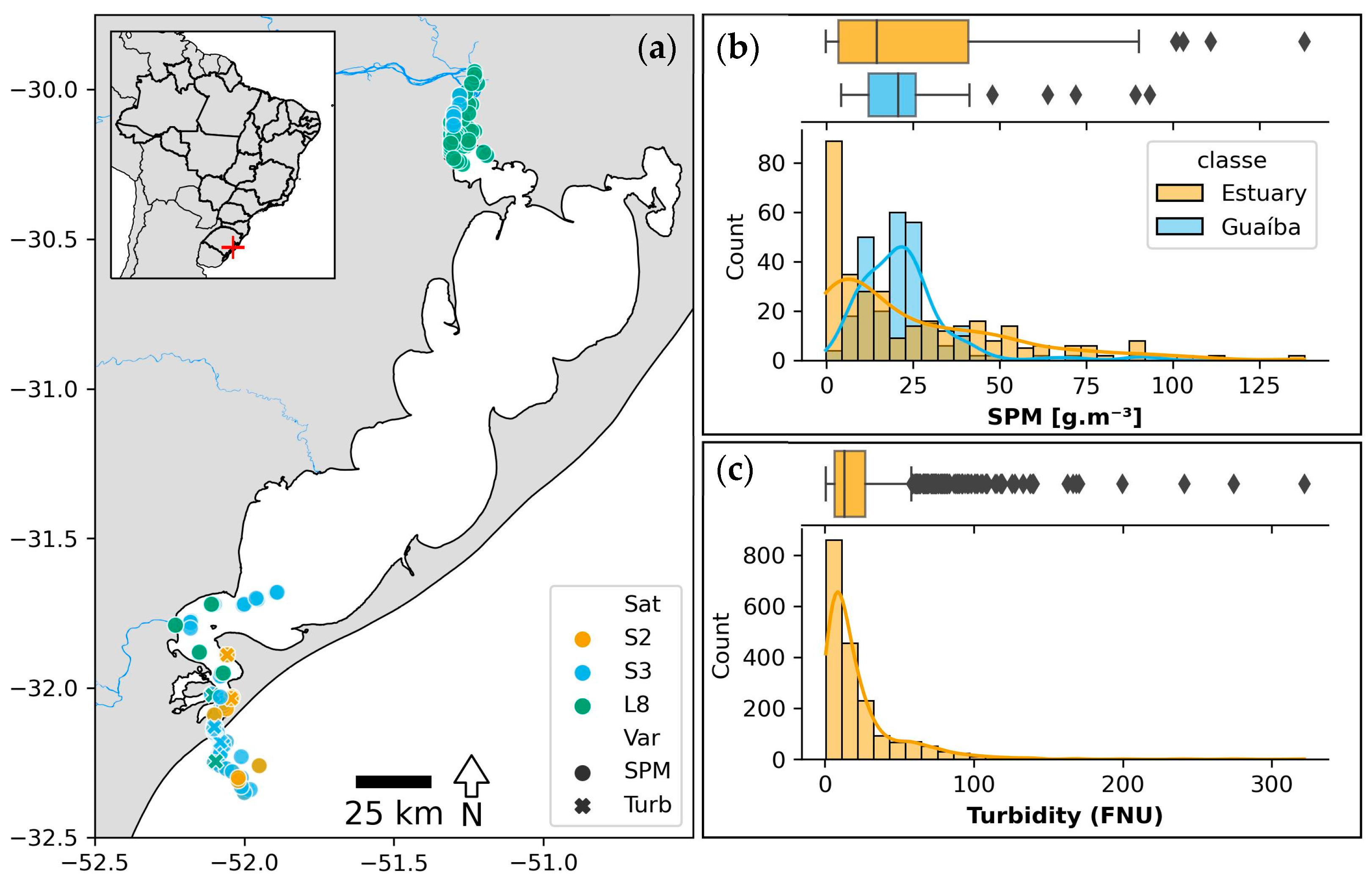
Patos Lagoon (Figure 1) is located on the southern coast of Brazil and is considered the world’s largest choked coastal lagoon [39]. It is approximately 250 km long and 40 km wide and connected to the South Atlantic Ocean through a single narrow channel (width <700 m). Circulation is driven by winds and river discharge, as the channel functions as a lowpass filter, attenuating tides [40]. At high river discharge (>2000 m3·s−1), the dynamics are controlled by the discharge, favoring freshwater flushing [41]. At low discharge (<2000 m3·s−1), the circulation is mainly controlled by winds. South quadrant winds generate saline water inflow, while north-quadrant winds generate outflow [41].
SPM enters the system through three main tributaries: the Guaíba River, Camaquã River, and São Gonçalo Channel (which connects Patos Lagoon to Mirim Lagoon) [42]. High-input periods (common in winter and spring, as well as in El Niño years) lead to higher SPM concentrations, with the entire lagoon becoming turbid [36,42]. Low-input periods (common in summer and autumn and in La Niña years) lead to lower SPM concentrations, with river plumes restricted to the mouths of tributaries [36,42]. The mean SPM concentrations are approximately 38 g·m−3 in the innermost portion of the lagoon and approximately 10 g·m−3 in the lower estuary [3].
Turbidity is one of the most important parameters for aquatic metabolism in the lagoon, altering light penetration and, thus, primary production [5]. A direct and linear relationship between turbidity and SPM has been observed in the region [43], allowing the use of turbidity as a proxy for SPM concentration. Furthermore, turbidity can be used to delimit Patos Lagoon coastal plumes using remote sensing [34]. Turbidity values in the Patos Lagoon estuarine zone usually range from 0 to 100 NTU but can exceed 300 NTU (Figure 1).
2.2. Data
2.2.1. In Situ Data
The in situ turbidity and SPM data for Patos Lagoon and the spatial and frequency distributions of the data are shown in Figure 1. In situ turbidity data were obtained from Brazilian Coast Monitoring System (SiMCosta; simcosta.furg.br/home) buoys RS1, RS2, and RS4 between 2016 and 2021. The buoys are located in the estuarine region of Patos Lagoon, and the 700 nm wavelength is used for measuring turbidity. Only data that passed the quality control tests (gross range test, spike test, rate of change test, and flat line test) were considered. This dataset was complemented by in situ turbidity measurements from various research projects in Patos Lagoon described in [44] (in preparation).
In situ SPM data were obtained from Távora et al. [45]. The database includes measurements conducted during different research projects between 1978 and 2019, covering the entire length of Patos Lagoon. The data passed quality tests [46], ensuring consistency. In this work, only measurements conducted in situ and close to the surface (depths up to 1 m) were considered.
2.2.2. Remote-Sensing Data
Scenes from satellites/sensors Landsat-8/Operational Land Imager (OLI), Sentinel-2 Multispectral Instrument (MSI), and Sentinel-3 Ocean and Land Color Instrument (OLCI), hereinafter referred to as L8, S2, and S3, respectively, were obtained for the study area (swaths between 30.00°S and 52.75°W and 32.75°S and 50.30°W), covering the 2013–2022, 2016–2022, and 2016–2022 periods, respectively. For S2, only scenes with cloud coverage lower than 10% and tiles containing matchups with in situ data were considered. For S3, only scenes that covered the entire study area were considered. For L8, all available scenes were used.
2.3. Methods
2.3.1. Atmospheric Correction
Satellite scenes were further processed for atmospheric correction using two distinct methods, namely, POLYMER [16] and ACOLITE dark spectral fitting (DSF) [17]. This choice was based on previous comparisons of these two methods, showing that they have distinct spectral uncertainties [11] and performances for different final products [25]. In Patos Lagoon, previous works have applied ACOLITE [10,42] and POLYMER [34], but without a direct comparison of these methods. Additionally, [10] lists the advantages and limitations of each correction. Both methods were developed for coastal regions, and the main difference is the approach used for estimating the aerosol contribution. While POLYMER uses spectral matching between a polynomial and bio-optical model [47], ACOLITE identifies pixels and bands with negligible water reflectance (Rw) values. Additionally, POLYMER can perform atmospheric correction even with sun glint. A 20 m resolution was used for S2 in both atmospheric correction methods.
2.3.2. Matchups
Regarding turbidity, matchups were selected based on a maximum time difference of 30 min between the satellite overpass and in situ data acquisition times. Regarding SPM, data obtained on the same day were considered matchups, as the database does not provide temporal information. For each matchup, a 3 × 3 pixel window was extracted near the coordinates of in situ measurements. Pixels marked as invalid using atmospheric correction flags, negative reflectance values, or quality water index polynomial (QWIP) scores >±0.3 were removed. The QWIP was developed by Dierssen et al. [48] and provides a metric for quality control of water reflectance data based on the apparent visible wavelength (AVW) [49] of diverse optical water types. Windows with a coefficient of variation (ratio of the standard deviation to the mean) greater than 0.2 and with less than 50% valid pixels (in this case, less than 5 pixels) were also excluded, following IOCCG recommendations [50]. The remaining windows were aggregated by the median, and the results were used in the turbidity and SPM algorithms. The number of available matchups depends on the atmospheric correction, algorithm, and band, ranging from 37 to 346 and from 18 to 101 for turbidity and SPM, respectively. The exact number of matchups for each combination is shown in Section 3.
2.3.3. Turbidity and SPM Algorithms
The turbidity algorithms used include those of Nechad et al. [9] and Dogliotti et al. [33] (hereafter referred to as N09 and D15, respectively), applied to the red (~665 nm for S2 and S3 and ~655 nm for L8) and near-infrared (~865 nm for the three satellites) bands. These algorithms were selected because they are widely applied in coastal regions and represent two distinct approaches: N09 is a single-band algorithm that may struggle with reflectance saturation, while D15 aims to contour saturation by switching between two bands (red and NIR). The N09 algorithm can be expressed as follows:
where T is the turbidity (in FNU), Rw is the water reflectance, and A and C are empirical coefficients defined by the author. The A coefficient is largely calibrated based on in situ measurements and controls the linear relationship between the reflectance and turbidity, while the C coefficient is generally calculated based on standard optical properties and defines the saturation limit without impacting the linear regime. Spectrally convoluted coefficients for each satellite sensor were used (Section 2.3.4).
The D15 algorithm is based on the same equation but uses a switching mechanism. For Rw values lower than 0.05, the algorithm uses the red band, while for Rw values higher than 0.07, the infrared band is used. Between these values, both bands are used, applying a linear weighting function within the reflectance range. The original coefficients provided by the authors were used.
To estimate the SPM concentration, the algorithms employed were those of Nechad et al. [27], Novoa et al. [2], and Távora et al. [29], which are hereafter referred to as N10, N17, and T20, respectively. The N10 and N09 algorithms use the same equation (Equation (1)) but with different values for the A and C coefficients (again, spectrally convoluted coefficients were used). The N17 algorithm was developed for the Gironde Estuary (France) and contains a switching mechanism. It uses a linear model with the green band for low reflectance values, a linear model with the red band for intermediate reflectance values, and a polynomial with the near-infrared band for high reflectance values. Each band receives varying weights depending on the water reflectance and saturation interval.
Finally, the T20 algorithm is also based on Equation (1) but considers all available bands above 600 nm (except for the range between 670 and 700 nm, due to the chlorophyll fluorescence signal). In addition to the SPM concentration, the uncertainties in the SPM estimates are provided. In this work, only the bands between 630 and 850 nm were used, as these bands improved the algorithm performance. T20 also requires the sea surface temperature (SST) as input. Data from other instruments of the same satellites could be used (such as the Thermal Infrared Sensor, TIRS, for L8), but they are not available for all satellites used (S2 does not provide an SST product). Therefore, the SST was obtained from the Climate Change Initiative (SST CCI) L4 product. The SST CCI product was developed by Merchant et al. [51] and provides SST data obtained from different satellite sensors. The L4 product has a spatial resolution of 0.05° × 0.05° with daily coverage, and it showed favorable agreement with the in situ SST data for Patos Lagoon (Figure A1). Because the spatial resolution of these images is coarser than that of the satellite sensors, the SST values for each pixel were assigned based on the closest value to the SST CCI data.
2.3.4. Convolution and Regional Recalibration Methods
The A and C coefficients (Equation (1)) provided for N09 and N10 [9,27] were convoluted through the relative spectral response (RSR) of the satellite sensors based on the protocol of Távora et al. [10] (https://github.com/julianatavora/High-resolution-satellites-primer-codes/tree/main/spectral_conv, accessed on 21 August 2023). This is an important step in adjusting the obtained coefficients via in situ radiometry to match the spectral characteristics of each satellite sensor.
Furthermore, to reduce the bias and better adjust the turbidity and SPM estimates for Patos Lagoon, a regional recalibration of the N09 and N10 coefficients was performed. Recalibration was performed using the GeoCalVal method [52], adapted for nonlinear models (Equation (1)). GeoCalVal allows calibration/validation datasets to be split objectively, creating different combinations of sets by using bootstrapping and jackknife sampling methods. As a result, the model provides the frequency distributions of the calibrated coefficients and validation metrics for different combinations of sets. The method was developed for the calibration and validation of geophysical observation models, and its applicability is not limited to the variables used here (SPM and turbidity) but extends to other cases (for example, to chlorophyll-a absorption and soil moisture, as in the paper that introduces the method [52]).
The median value of coefficient A (Equation (1)) and the statistical parameters (Section 2.3.5) were calculated. The C parameter in Equation (1) was fixed at the convolved value for the S3A satellite (Table 1). Fixing the C value has been shown to improve performance. This could be explained by the fact that this coefficient controls the saturation limit, as we did not observe a complete saturation curve in our data (Figure A2). To allow before-and-after comparison, the N09 and N10 algorithms using the original coefficients were also evaluated following the same method (i.e., using the same validation sets). The win rate (shown below) was calculated after calibration and validation using the entire dataset.
2.3.5. Statistical Parameters
Based on Seegers et al. [53], five statistical parameters were used to evaluate the performance of the different combinations of atmospheric corrections and turbidity/SPM algorithms: Kendall’s tau correlation coefficient, root-mean-square error (RMSE), mean absolute error (MAE), mean absolute percentage error (MAPE), and bias.
where n is the number of matchups for each algorithm and y and ŷ are the measured and estimated variables (turbidity or SPM), respectively.
The win rate (WR) was also used as a statistical parameter because it directly compares residuals and provides a way of classifying algorithm performance [53,54]. For each pair of algorithms, the winning percentage was calculated (one algorithm receives a win when its residual is lower than that of the other). This process was performed for all algorithm combinations. Finally, the WR of each algorithm was obtained as the average winning percentage between all combinations. For a given Algorithm A, WR can be expressed as follows:
where is the number of combinations with two elements that contain Algorithm A, m is the number of algorithms, A and B are two different algorithms, n is the number of simultaneous matchups between A and B, and the residual is the difference between the algorithm estimate and in situ measurement.
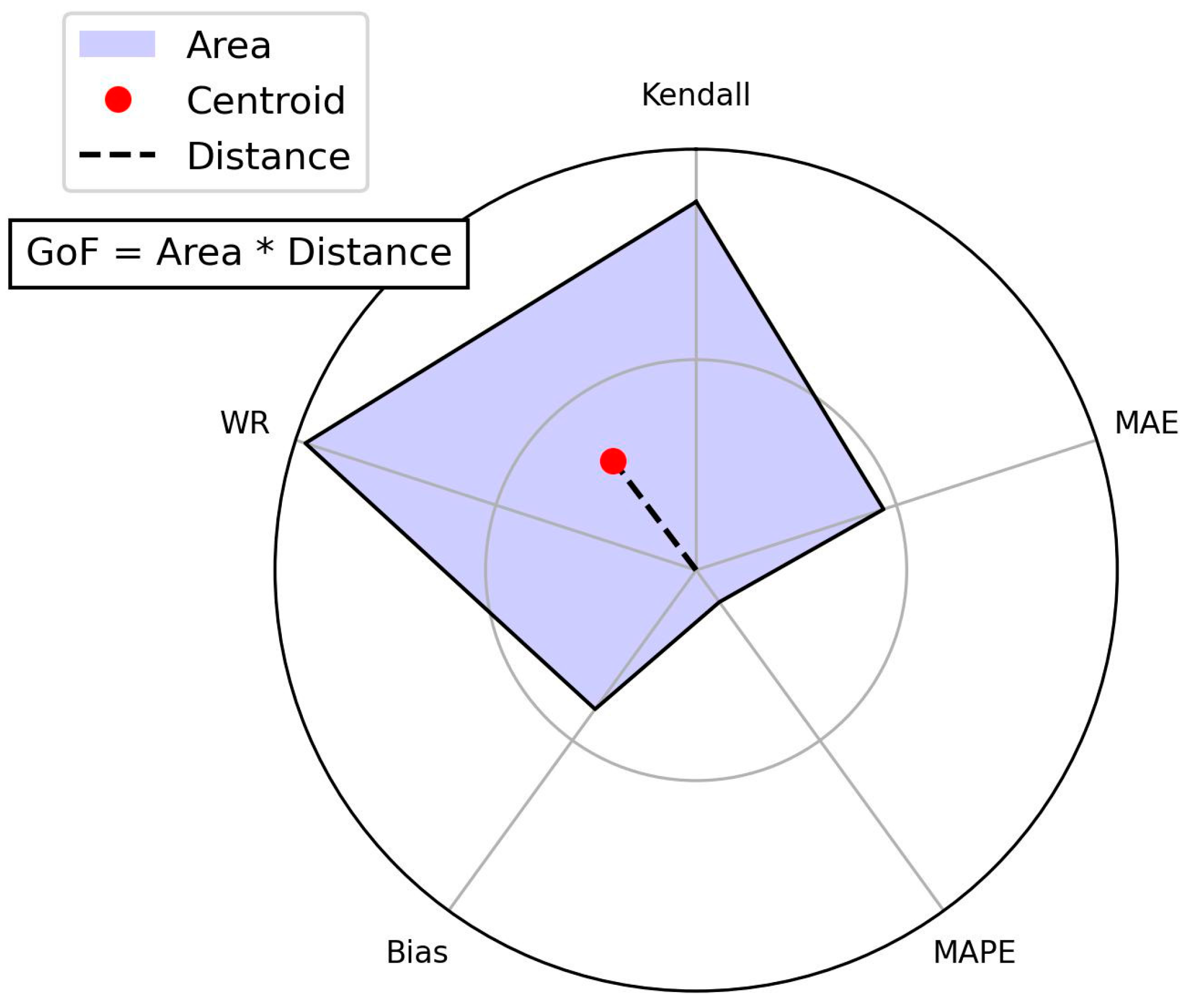
Given the diversity of metrics and ways to rank the performance, a robust alternative is to use radar plots to calculate the area associated with each approach [55]. Here, we adopted the product between the radar plot area and the distance between the centroid and plot center as a metric of the goodness of fit (GoF), as shown in Figure 2. This new metric (hereafter referred to as GoF) favors both the best overall performance (smallest area) and the most balanced performance (the centroid is closest to the center). The selected statistical parameters considered by GoF provide metrics for correlation (nonparametric Kendall correlation coefficient), accuracy (MAE and MAPE, given absolute and relative errors, respectively), bias (allowing identification of over- or underestimation), and comparative performance (WR, pairwise comparison of the residuals). The RMSE was not considered, to avoid redundancy with the MAE, because it is not designed for nonnormal statistical distributions [53]. All the parameters were scaled between 0 (best performance) and 10 (worst performance) based on values close to the minimum and maximum (Kendall = [0, 1], MAE = [0, 60], MAPE = [0, 800], bias = [0, 60], and WR = [0, 100]). Thus, the lowest GoF values indicate the best combination of atmospheric correction and algorithm for each remote-sensing product. The specific formulas applied to calculate GoF are those of the statistical parameters (Equations (3)–(6)), the area and centroid of a polygon, and the feature scaling of the parameters. Thus, GoF can be applied to any comparison between measured and estimated data (including other optical remote-sensing products and chlorophyll-a and CDOM). The Supplementary Material provides a Python script to estimate GoF using some example data.
3. Results
3.1. Performance of the Different Combinations of Atmospheric Corrections and Algorithms
The spectral convoluted coefficients from N09 and N10 for the L8, S2, and S3 satellites and the red and NIR bands are provided in Table 1.
The statistical parameters for each of the satellites, atmospheric corrections, and turbidity algorithms are shown in Figure 3 (the radar plots are shown in Figure A3). The best performance was associated with percentage uncertainties (measured via MAPE) between 27% and 42%, with MAE values between 10 and 11 FNU. The MAPE allows us to rank the algorithms based on the normalized accuracy, which does not occur with the MAE. In cases with higher (lower) in situ concentrations, it is expected that the errors measured by the MAE will also be greater (less). For the three satellites, the best combination of atmospheric correction and algorithm (according to MAPE) was POLYMER and N09, differing only in the band used (655 nm for L8 and 865 nm for S2 and S3).
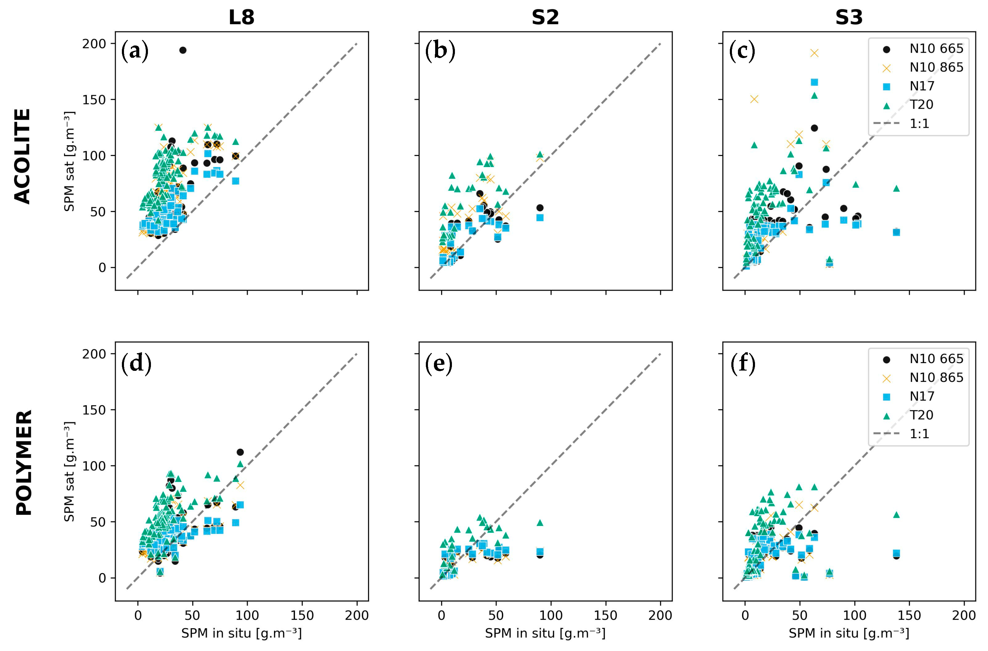
The performance of the SPM algorithms is shown in Figure 4 (refer to Figure A4 for the radar plots) and was, in general, not as satisfactory as that of the turbidity algorithms. The lower MAPE for each satellite varied between 68% and 81%, with MAE values between 10 and 12 g·m−3. Again, the best combination (according to MAPE) was POLYMER atmospheric correction and a single-band algorithm (N10, with the 865 nm band for L8, the 665 nm band for S3, and the same performance for the S2 bands).
The win rate (WR) offers another way to rank the performance (as in Pahlevan et al. [11]) through the direct comparison of the residuals. Regarding turbidity and SPM, the best WR was assigned to the same combination as for the MAPE (POLYMER and N09; POLYMER and N10). As an exception, the best performance changed for S2, from N09 and N10 to D15 and N17, respectively. Additionally, the best band for S3 ranged from 665 to 865 nm, corresponding to the same WR values as those for D15 and N17. The differences between the best performance values of MAPE and WR reflect the distinction between comparing the algorithms with all the estimates (as via MAPE) and only in cases where both have valid results (as via WR). WR does not consider the amplitude of the residuals, so a high WR value can be related to a high MAPE value in cases where the algorithm performs well in most cases but fails and exhibits large errors in a few cases. For S2 and S3, the high WR for the band-switching algorithms (D15 and N17) indicates the efficiency of this mechanism in choosing the ideal band for each reflectance interval in most cases, as it aims to avoid saturation and benefits from the better sensibility of shorter (longer) wavelengths to lower (higher) turbidity and SPM values [56]. Additionally, this advantage may be more notable in cases with higher turbidity and SPM variability, as observed in the Patos Lagoon estuary, which constitutes most of the matchups for S2 and S3 (Figure 1).
In addition to the MAPE and WR, it is important to measure the degree of under- or overestimation by the bias. The algorithms using POLYMER underestimated turbidity (negative bias), while the algorithms using ACOLITE overestimated turbidity (positive bias, except for S3), as shown in Figure 5, where the estimates using POLYMER (ACOLITE) are usually below (above) the 45° line. This pattern was not clearly observed for the SPM algorithms (Figure 6), which may reflect the theoretical differences between these two variables, as turbidity does not depend only on the SPM concentration but also on the size, composition, and shape of particles. Figure 6c,f also show large errors for SPM estimates using the S3 satellite and N10, N17, and T20 algorithms. This is possibly caused by the adjacency of land pixels and the sensor’s lower spatial resolution, as discussed in Section 4.2.
Regarding T20, almost all the metrics showed high uncertainty when using ACOLITE (Figure 4), with the SPM concentration overestimated when using this atmospheric correction (Figure 6). This could be attributed to the broader range of bands used by T20 to estimate SPM, as the spectral uncertainty in the atmospheric correction procedure can propagate and lead to unrealistic results when algorithms that depend on several bands are applied (as in the classification of optical water types [20]). POLYMER and ACOLITE represent two distinct approaches (spectral matching and dark spectral fitting, respectively) that may lead to different atmospheric correction spectral errors (as described by [22]). For Patos Lagoon, the results obtained using POLYMER and T20 (Figure 4) suggest that this atmospheric correction provides more realistic spectra, with lower uncertainty in Rw and better SPM estimates than those of ACOLITE.
The different statistical parameters led to different interpretations of the best combination of atmospheric correction, algorithm, and band (Figure 3 and Figure 4). This task was simplified by analyzing the GoF metric, which provides a summary of the selected parameters (Figure 2). Table 2 lists the best combinations for estimating turbidity and SPM based on GoF; these combinations were mostly associated with POLYMER, except for SPM estimates using S2.
3.2. Regional Recalibration of Coefficients
The validation statistical parameters for turbidity and SPM are shown in Figure 7 and Figure 8, respectively (the radar plots are shown in Figure A5 and Figure A6, respectively). The recalibrated A coefficients for all satellites (L8, S2, and S3), atmospheric corrections (ACOLITE and POLYMER) and bands (665 and 865 nm) are listed in Table A1.
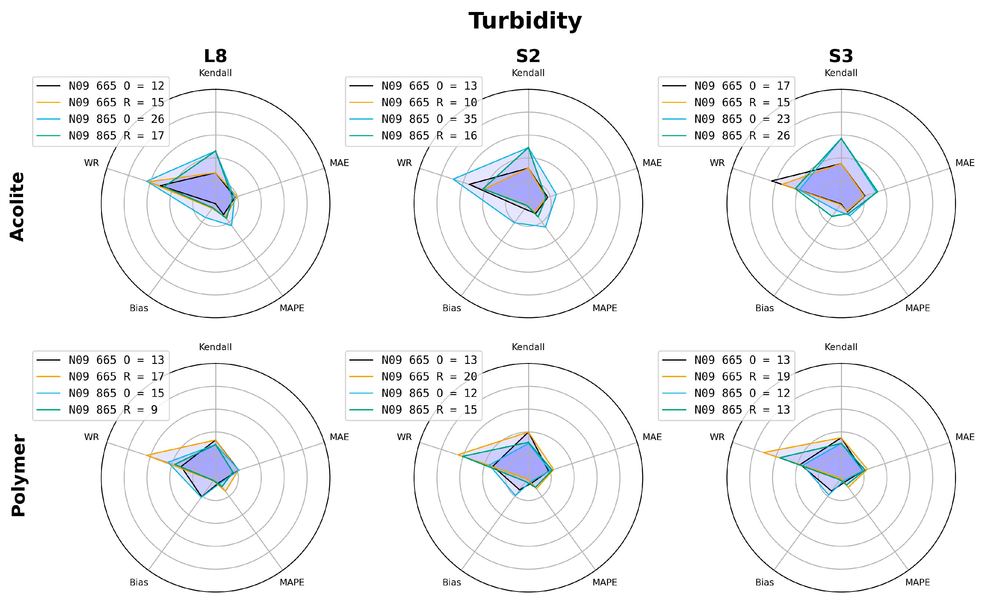
The turbidity test results indicated that for five of the cases, recalibration led to better performance (lower GoF value in Figure 7). In general, this improvement was not followed by a change in the accuracy (RMSE, MAE, and MAPE) of the algorithms but rather a reduction in bias. This phenomenon is shown in Figure 9, where the estimates (especially those using POLYMER) are closer to the 1:1 line.
However, for seven of the combinations, the GoF metric shown in Figure 7 increases after recalibration, which could be attributed to a better fit for high- or low-turbidity data points. As the GeoCalVal method samples from the full range and the lowest values represent most of the data (refer to the data points with a turbidity lower than 40 FNU in Figure 9), an expected result is that the final coefficient is better suited for estimating the lowest values. This led to a worsening in the estimates of the highest turbidities, causing the GoF value to increase for the S3-ACOLITE-N09-865 nm combination (Figure 7). However, this was not the case for most combinations because the high turbidity data points pushed the least square fit toward higher coefficients. In this way, the performance decreased at the lowest turbidities but improved at the highest turbidities. As a result, for most of the cases shown in Figure 7, the GoF metric increases after recalibration, indicating that this approach was ineffective at improving the turbidity estimates in these cases.
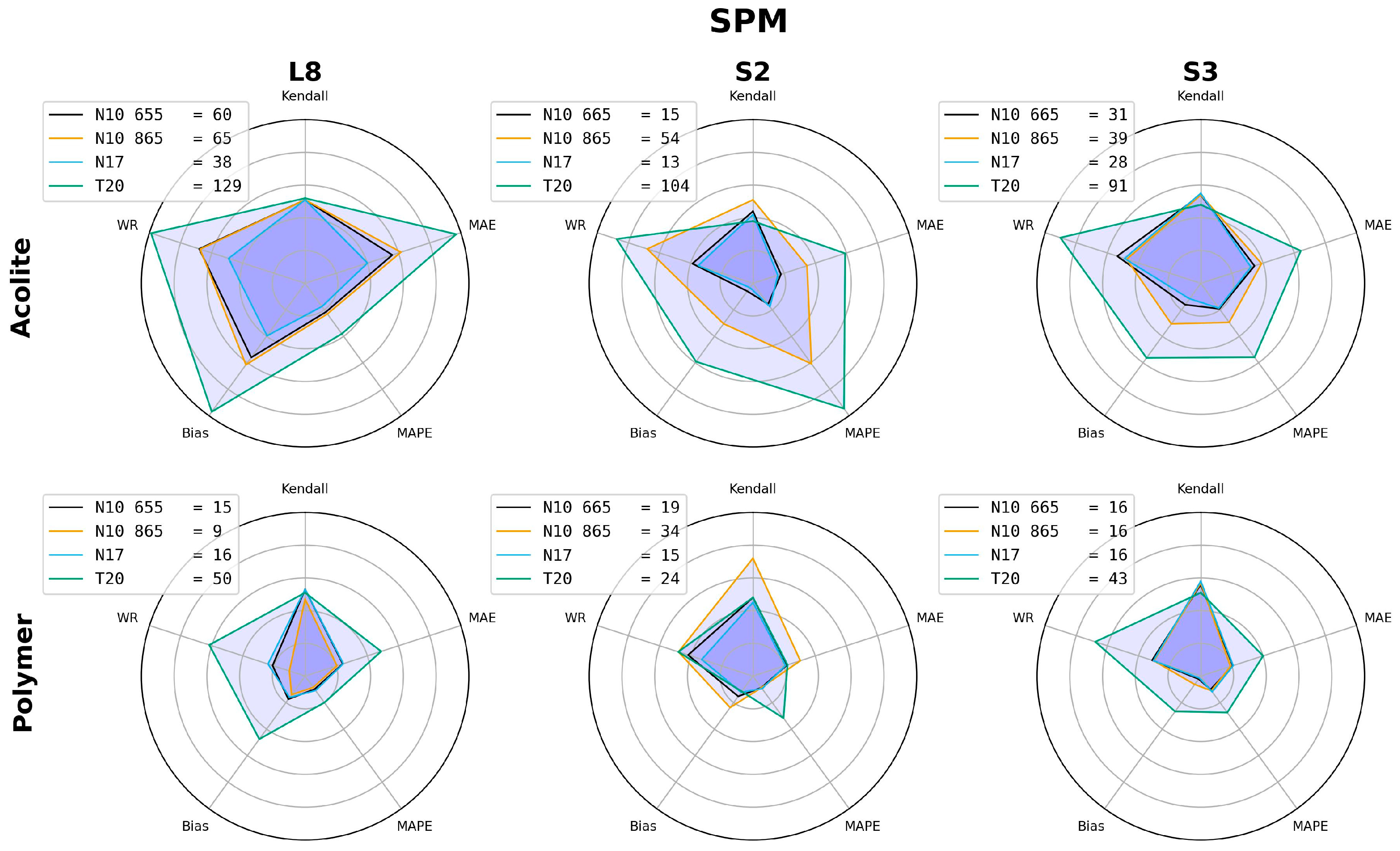
However, with regard to the SPM estimates, recalibration led to improvements in the performance of most of the algorithms (Figure 8) and the estimates were closer to the 1:1 line (Figure 10). As an exception, the S3-POLYMER-N10-665 nm combination did not yield an improvement. Nevertheless, in this case, the performance was the same as that before recalibration. This is associated with the same pattern described previously, with a better fit at low SPM concentrations.
Table 3 lists the recommended combinations of atmospheric corrections, bands, and coefficients for estimating turbidity and SPM in Patos Lagoon. The SPM algorithm provided an encouraging result in terms of recalibration: the regionally recalibrated coefficients (shown in bold font in Table 3) provided better results than the original coefficients in all the cases. Despite the better performance of N17 for S2 (Table 2), the N09 algorithm was recommended (Table 3) because it provided similar values for the statistical parameters but a lower MAPE value.
Figure 11 shows the mean SPM concentration in the Patos Lagoon estuary based on all S2 scenes, ACOLITE atmospheric correction, the N10 algorithm, and the red band (665 nm). The concentrations obtained using the original coefficients (Figure 11a) were consistently higher than those obtained with the recalibrated coefficients (Figure 11b). If we consider an optical depth of 1 m for the red band (as in [56]), then the total SPM mass (sum of the concentration of all pixels multiplied by the pixel volume) is 2.78 × 10⁴ tons and 2.33 × 10⁴ tons for the original and recalibrated coefficients, respectively. This resulted in a difference of 4.53 × 10³ tons, illustrating the impact caused by not regionally calibrating the coefficients, especially considering the importance of SPM in coastal management.
4. Discussion
4.1. Previous Studies of Patos Lagoon and Results without Regional Recalibration
Previous studies on turbidity in Patos Lagoon based on remote sensing focused on applying algorithms to study the plume [34,57] and water quality in the region [10]. For the L8 and S2 satellites, POLYMER atmospheric correction and N09-recalibrated coefficients [34] achieved better performance in the NIR band (based on Kendall’s tau correlation coefficient). Compared to [10], who used Landsat 5, 7, 8, and 9 satellites and ACOLITE atmospheric correction, the results of [34] indicated that POLYMER yields better performance for Patos Lagoon. In this study, the GoF metric was applied and the best performance for estimating turbidity was associated with POLYMER atmospheric correction and the NIR band, following these studies.
Regarding SPM, previous works focused mainly on its dynamics in the region, investigating its variability as a function of circulation [58], wind and river discharge [3], interannual variability associated with ENSO cycles [36], and input from tributaries [42]. Two of these studies focused on evaluating SPM algorithms for the region.
Bortolin et al. [42] evaluated the performance of SPM estimates using Landsat 5, 7, and 8 satellites, ACOLITE atmospheric correction, and the T20 algorithm. Based on the same database used in this study [45], the authors obtained RMSE = −37 g·m−3 and MAPE = 79. This performance was better than that obtained in this study for L8 (RMSE = 60 g·m−3, MAPE = 305%), showing underestimation of the SPM concentration (in contrast to the overestimation found here). This could be explained by the methodological differences involved, especially the larger number of matchups used here (n = 98 vs. n = 47 for Bortolin et al.), which led to greater (and more realistic) optical and SPM variability, a more challenging estimate, and, thus, poorer performance. Additionally, differences between the studies regarding the versions of ACOLITE, sources of sea surface temperature data (important to the T20 algorithm for estimating water absorption), and sensors may cause these differences.
Távora et al. [36] used the Aqua/MODIS satellite and compared three SPM algorithms (N10, N16, and HAN16 [38]), with atmospheric correction from [37]. Their results indicated that the best performance was associated with switching the band algorithms (N17 and HAN16). Among the multiband algorithms, N17 was identified as the best (RMSE = 14.6 g·m−3 and MAPE = 36.9%). In this study, the N17 algorithm was identified as the algorithm with the best performance for S2 using ACOLITE. However, Távora et al. reported a better performance than that obtained in this study using S3, which has spatial and temporal resolutions closer to those of Aqua/MODIS (RMSE = 22 g·m−3 and MAPE = 95%) for the S3-POLYMER-N17 combination. Távora et al. used a much larger dataset (n = 1241 against n = 69 used here), which was mainly obtained from turbidity in situ measurements and converted into SPM. As turbidity can be more easily estimated (compared to SPM, Figure 3 and Figure 4), this difference may explain the better performance. Again, differences related to the atmospheric correction, sensors, temporal coverage, and matchup selection (especially the window size and maximum time and distance difference allowed) may also have contributed to the findings.
Moreover, the spatial variability in the algorithm performance cannot be overlooked. Both Bortolin et al. [42] and Távora et al. [36] reported higher accuracy (lower RMSE and MAPE) for the Guaíba region. Távora et al. [36] showed that different algorithms performed better in the estuarine (HAN16) and Guaíba (N17) regions, with larger differences between the algorithms in the central part of the lagoon (reaching approximately 10 g·m−3). The central region of Patos Lagoon represents a data gap in this study (Figure 1). The lack of information is one of the issues in the study area, with a large number of studies focusing on the estuarine region but only a few focusing on the limnic portion [59].
4.2. Regional Recalibration and Sources of Uncertainty
The results before recalibration showed an unsatisfactory performance for the algorithms in the study area. We addressed this poor performance by regionally recalibrating the empirical coefficients of N09 and N10, leading to bias reduction, although a trade-off between MAE and bias was observed. The need for recalibrating coefficients may be associated with uncertainties in atmospheric correction (as orbital data were used here) and the optical properties of Patos Lagoon (which may differ from those used during the calibration of the original coefficients).
Adjacency effects are associated with surfaces with contrasting reflectance, where photons from the higher reflectance surface (usually the land) are scattered into the instantaneous field of view (IFOV) of the sensor, mixing with the signal from the lower reflectance surface (usually water) [60]. This effect depends upon the characteristics of the atmosphere (aerosol optical depth), the target (water reflectance), and the background (land cover’s albedo) [60,61,62]. Paulino et al. [62] evaluated adjacency effects on Brazilian inland waters, showing that this effect is relevant for distances between 0.1 and 2 km from land. On the other hand, Bulgarelli and Zibordi [61] observed adjacency effects up to a few tens of kilometers from the coast. According to them, adjacency introduces a bias into remote-sensing reflectance, with a magnitude that depends on the atmospheric correction applied. For ACOLITE, adjacency effects could cause an overestimation of the SPM concentration, as already observed by Renosh et al. [26] for the Gironde Estuary due to the proximity between land pixels and automated turbidity stations. This approach is relevant considering the narrow channel that connects Patos Lagoon to the Atlantic Ocean (Figure 1). Regarding POLYMER, the atmospheric correction is based on the residual between Rw (given by a bio-optical model) and the Rayleigh-corrected reflectance [16]. This approach aims to correct for sun glint, but adjacency effects are also included in the residual and can thus be corrected via POLYMER [23]. In contrast, the underestimation of turbidity and SPM by POLYMER may reflect the restriction imposed by its bio-optical model [22]. In the present work, turbidity and SPM estimates using the NIR band (865 nm) were not systematically overestimated, as would be expected in the presence of adjacency effects [62]. Hence, one may consider that adjacency did not significantly affect the estimates.
Nevertheless, Figure 6c,f showed large errors for SPM estimates using the S3 satellite and N10, N17, and T20 algorithms. Most of the under- or overestimated points in Figure 6c,f are from the channel that connects Patos Lagoon to the ocean (Figure 1), suggesting that these points may be affected by the adjacency of land pixels. The S3 spatial resolution (300 m) contributes to this explanation, given that the narrowest part of the channel is 500 m wide and the matchups were extracted using a 3 × 3-pixel window. This effect was less evident for the POLYMER atmospheric correction (Figure 6f), for which two possible reasons arose: (i) POLYMER might have corrected for adjacency effects [23]; (ii) some of the matchups using POLYMER were excluded based on the quality control flags (invalid pixels, large window variability, negative water reflectance, and QWIP).
The effect of the sensors’ spatial resolutions (20, 30, and 300 m, respectively, for S2, L8, and S3) on the accuracy of the estimates was not investigated here, as it would involve isolating the effect of spatial sampling. The study of Pahlevan et al. [63], for example, found differences of up to 18% in the reflectance obtained from sensors with distinct spatial resolutions (OLI, MODIS, and VIIRS). According to the authors, this can be attributed to the footprint size (and associated sensor viewing angle) and to in-water variability. Dorji and Fearns [64] studied turbid waters in northern Western Australia and found that the in-water variability may cause an underestimation of SPM concentration by lower resolution sensors (such as MODIS) due to intrapixel variability. On the other hand, Luo et al. [12] found overestimated turbidity estimates in lower-resolution sensors in the Gironde Estuary, caused by pixel contamination by land and muddy shallow waters. These results show that the bias introduced by the spatial resolution differences depends on the target’s background (i.e., the water variability around the in situ measurements).
The atmospheric corrections with a better performance were not always the same for the red and NIR bands, which could be explained by the spectral errors of each method [22]. This introduces additional complexity to the choice of the best atmospheric correction, especially for band-switching algorithms (D15 and N17). Renosh et al. [26] faced the same problem in the Gironde Estuary, obtaining a better performance associated with different corrections for the red and NIR bands for S3. The authors used the N17 algorithm and chose the atmospheric correction with better performance in the NIR band, since most of the SPM range in the study area was estimated using this band.
Regarding optical properties, algorithms commonly assume a fixed value for specific backscattering coefficients [9,27]. However, this coefficient varies according to the size, shape, and composition of particles [31]. In some cases, as observed by Mabit et al. [24] in Québec coastal waters, there may be an inverse relationship between the mass-specific coefficient and SPM concentration, rendering remote-sensing estimates of SPM unfeasible. For Patos Lagoon, this variability is probably associated with differences in the characteristics of the material supplied by its tributaries. This explains the spatial variability in the algorithm performance observed in previous studies. Variability in the structure of phytoplankton communities [65] and in the production of particulate material by these organisms [66] may also be relevant factors. Organic particles, for example, have been associated with lower backscattering coefficients in other regions (e.g., in the Artic Ocean [67]). The influence of CDOM on SPM estimates should also be considered. Although its effect at longer wavelengths is often considered negligible [27], Mabit et al. [24] reported a positive correlation between the residuals of an SPM algorithm and CDOM absorption, with an increase (decrease) in CDOM absorption associated with an underestimation (overestimation) of the SPM concentration. However, their study revealed a case with a low SPM concentration (mostly less than 10 mg·L−1), and CDOM optically dominated waters.
The saturation of Rw at high turbidity and SPM concentrations is another challenge facing algorithms [32]. In theory, the absence of saturation in the data (Figure A2) favors the use of single-band algorithms (as in [24]), while moderate SPM concentrations (between 10 and 60 g·m−3; Figure 1) favor the use of the red band (the ideal bands for each concentration interval are reported in [56], a study of the Rhone River and its plume). In this study, the best performance was obtained with single-band algorithms (N09 and N10). However, the red band did not perform better than the NIR band, possibly revealing the influence of high turbidity and SPM values on statistical parameters.
Within this context, the RMSE values were consistently greater than the MAE values. The RMSE is not recommended for cases where the data are not normally distributed, which may lead to an underestimation of the algorithm performance [53,68]. Regarding the S3 turbidity estimates (Figure 3 and Figure 5), a group of data points with high turbidity and low reflectance amplified the negative bias of the N09 algorithm estimates, causing an increase in the values of several parameters (RMSE, MAE, and MAPE). Additionally, the various statistical parameters led to different results for the best performers for each satellite. A novel GoF metric (Figure 2) was proposed here and was shown to be a reliable answer to this problem, allowing objective classification of the performance. Thus, this metric is recommended for future studies and can be directly applied to other algorithms and regions. Attention must be given to the normalization of statistical parameters (maximum and minimum values considered), as the resultant polygon is sensitive to these values.
We also highlighted the importance of using the GeoCalVal method. Regarding S2 and SPM, only a few matchups were available. A simple calibration approach (randomly splitting the data into fractions of 70% and 30% as calibration and validation datasets, respectively) could lead to high uncertainty in the calibrated coefficients (different datasets could yield different results). GeoCalVal, however, provides the opportunity to analyze all combinations. For N09 and N10, the statistical parameters obtained using the entire dataset (Figure 3 and Figure 4, respectively) were very close to those obtained using GeoCalVal (Figure 7 and Figure 8, respectively), indicating the robustness of the method.
However, there are still uncertainties that remain unidentified. An ideal scenario would be to use in situ radiometric data to directly evaluate atmospheric corrections and measure optical properties in the study area. Theenathayalan et al. [25] studied Vembanad Lake and suggested the following possible path: the low availability of field data was overcome by using a simulated reflectance dataset for the study area based on a radiative transfer model. The data were used to develop regional algorithms for chlorophyll-a and SPM concentrations, which outperformed previously established algorithms. Unfortunately, this approach relies on in situ reflectance and optical property data (absorption and scattering) to calibrate the radiative transfer model, which were unavailable in this study.
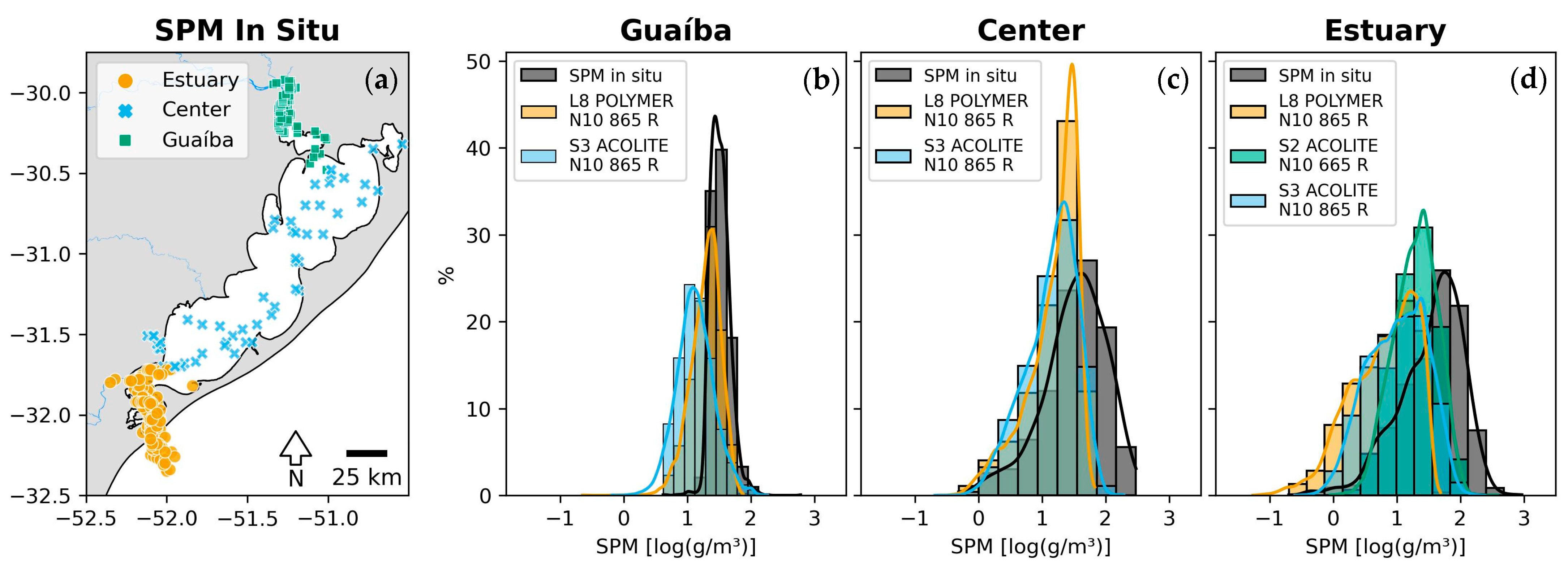
Differences in the performances of SPM algorithms between Patos Lagoon’s South and North parts (Guaíba and Estuary in Figure 1, respectively) had already been observed in previous works (as discussed in Section 4.1); they affect the regional recalibration of the coefficients. Figure 12 shows the SPM frequency distribution of all available in situ and satellite derived data (including those that are not matchups), estimated using the best combination for each satellite (Table 3). For optimally adjusted estimates, the distributions should show a similar pattern (e.g., [10]). However, the distributions in Figure 12 do not match exactly, indicating differences regarding the characteristics of the particulate matter throughout Patos Lagoon. A robust alternative would be to locally recalibrate the coefficients, treating the Guaíba and estuarine regions (Figure 1) independently, but the number of available matchups in the present work is insufficient (0 to 94 for the Guaíba, and 7 to 59 for the estuary). For the central portion, all available in situ SPM data are from before 2013 and, therefore, before the satellites were launched (2013 for L8, 2015 for S2A, and 2016 for S3A). Patos Lagoon is part of a long-term monitoring project [69], and the SiMCosta program provides measurements taken by moored buoys, but these data are limited to the estuary and the number of measurements synchronous to the satellites’ overpasses is still small. This limitation could be overcome by continuous and spatially distributed monitoring along the lagoon continuum. The Gironde Estuary is a positive example, with high-frequency water quality measurements taken by the MAGEST program [70] being useful for ocean color studies [12]. Automated stations for radiometric data acquisition (such as the AERONET-OC [71]) and global in situ datasets (such as GLORIA [72]) are also alternatives, but some regions (including Patos Lagoon) might be undersampled. Moreover, the large dimensions of Patos Lagoon (about 250 km long) and the financial difficulties found in developing countries currently limit a more complete evaluation of remote-sensing estimates.
Although multiple sensors were used (L8/OLI, S2/MSI, and S3/OLCI), an integration and intercomparison exercise was not one of our goals. Several approaches exist for data merging to reduce the systematic bias between sensors [73], which is fundamental for building climate records [74]. A simple and effective method is to match the cumulative distribution function (CDF) of satellite and in situ data, as used for satellite soil moisture estimates [75]. This is another possible future step for Patos Lagoon, especially considering the potential impact of climate change on coastal environments [76].
5. Conclusions
In this work, different combinations of atmospheric corrections and bio-optical algorithms for turbidity and SPM in Patos Lagoon were evaluated. The main conclusions are as follows:
- Based on the newly proposed GoF metric, the best algorithm performance was generally linked to POLYMER atmospheric correction, single-band algorithms (N09 and N10), and the NIR band (865 nm), with percentage errors (MAPEs) between 27% and 42% for turbidity and between 68% and 81% for SPM;
- Regional recalibration of the empirical coefficients for N09 and N10 led to a reduction in bias. We recommend the use of recalibrated coefficients for estimating the SPM concentration in Patos Lagoon via remote sensing. For turbidity, the original coefficients yielded a better performance for S2 and S3;
- The method used for recalibrating the coefficients (GeoCalVal) and the metric used to rank the performances (GoF) can be directly applied to other regions and optical remote-sensing products;
Future studies should focus on using field radiometric data, allowing the direct evaluation of atmospheric corrections and a better understanding of the optical variability of Patos Lagoon. The use of radiative transfer models is also a suitable alternative for filling these gaps, and merging data from multisensor climate records may provide important information on the impact of climate change in the region.
Supplementary Materials
The following Supplementary Material is available online from https://github.com/rafael-simao/GoF: a Jupyter Notebook with code in Python to estimate the goodness of fit (GoF) metric using some example data.
Author Contributions
Conceptualization, R.S., J.T., M.S.S. and E.F.; Data curation, R.S. and J.T.; Formal analysis, R.S.; Funding acquisition, E.F.; Investigation, R.S. and J.T.; Methodology, R.S., J.T., M.S.S. and E.F.; Project administration, J.T., M.S.S. and E.F.; Resources, E.F.; Software, R.S., J.T. and M.S.S.; Supervision, J.T., M.S.S. and E.F.; Validation, R.S., J.T., M.S.S. and E.F.; Visualization, R.S., J.T., M.S.S. and E.F.; Writing—original draft, R.S., J.T., M.S.S. and E.F.; Writing—review and editing, R.S., J.T., M.S.S. and E.F. All authors have read and agreed to the published version of the manuscript.
Funding
The authors are grateful to the LOAD Project—Long-Term Analysis of Suspended Particulate Matter Concentrations Affecting Port Areas in Developing Countries (ONR grant N62909-19-1-2145); the SUNSET Project—South Brazilian Shelf Sediment Transport: Sources and Consequences (CAPES/COFECUB, Process 88887.192855/2018-00); and the Dutch Research Council (NWO) under the SPARKLES project (NWA.1507.21.001, Grant number 16422) for sponsoring this research. Elisa Helena Fernandes is a CNPq research fellow (PQ2 No 304684/2022-8). Rafael A. Simão was supported by a CNPq Master’s scholarship, process No. 131424/2022-0. We thank the resources provided by CAPES to support the Graduate Program in Oceanology at FURG.
Data Availability Statement
The original contributions presented in the study are included in the article and supplementary material, further inquiries can be directed to the corresponding author.
Acknowledgments
The authors are grateful to SiMCosta for readily providing turbidity data for the Patos Lagoon Estuary, to USGS/NASA for the Landsat-8 imagery, to ESA for the Sentinel-2 and Sentinel-3 imagery, to RBINS for the ACOLITE atmospheric correction, and to HYGEOS for the POLYMER atmospheric correction. We also thank the Laboratório de Oceanografia Costeira e Estuarina (LOCOSTE) of the Universidade Federal do Rio Grande (FURG) for supporting this research.
Conflicts of Interest
The authors declare no conflicts of interest.
Appendix A. Additional Plots and Tables
Figure A1.
Time series of the sea surface temperature (SST) of Patos Lagoon based on in situ measurements (SiMCosta buoys) and reanalysis data (SST CCI L4 product).
Figure A1.
Time series of the sea surface temperature (SST) of Patos Lagoon based on in situ measurements (SiMCosta buoys) and reanalysis data (SST CCI L4 product).

Figure A2.
Optical saturation based on the NIR (x-axis) and red (y-axis) reflectance. The red line denotes the fitted regression between these two bands (as in [32]).
Figure A2.
Optical saturation based on the NIR (x-axis) and red (y-axis) reflectance. The red line denotes the fitted regression between these two bands (as in [32]).

Figure A3.
Radar plots of the statistical parameters for the turbidity estimates. The number after each algorithm and band denotes the area of the associated polygon. The best performance (smaller area) occurs closer to the center.
Figure A3.
Radar plots of the statistical parameters for the turbidity estimates. The number after each algorithm and band denotes the area of the associated polygon. The best performance (smaller area) occurs closer to the center.

Figure A4.
Radar plots of the statistical parameters for the SPM estimates. The number after each algorithm and band denotes the area of the associated polygon. The best performance (smaller area) occurs closer to the center.
Figure A4.
Radar plots of the statistical parameters for the SPM estimates. The number after each algorithm and band denotes the area of the associated polygon. The best performance (smaller area) occurs closer to the center.

Figure A5.
Radar plots of the statistical parameters for the turbidity estimates using the original (O) and recalibrated (R) coefficients. The number after each algorithm and band denotes the area of the associated polygon. The best performance (smaller area) occurs closer to the center.
Figure A5.
Radar plots of the statistical parameters for the turbidity estimates using the original (O) and recalibrated (R) coefficients. The number after each algorithm and band denotes the area of the associated polygon. The best performance (smaller area) occurs closer to the center.

Figure A6.
Radar plots of the statistical parameters for the SPM estimates generated using the original (O) and recalibrated (R) coefficients. The number after each algorithm and band denotes the area of the associated polygon. The best performance (smaller area) occurs closer to the center.
Figure A6.
Radar plots of the statistical parameters for the SPM estimates generated using the original (O) and recalibrated (R) coefficients. The number after each algorithm and band denotes the area of the associated polygon. The best performance (smaller area) occurs closer to the center.


Table A1.
Recalibrated A coefficients for turbidity (N09 algorithm) and SPM (N10 algorithm) for each combination of satellites (L8, S2, and S3), atmospheric corrections (ACOLITE and POLYMER), and bands (665 and 865 nm).
Table A1.
Recalibrated A coefficients for turbidity (N09 algorithm) and SPM (N10 algorithm) for each combination of satellites (L8, S2, and S3), atmospheric corrections (ACOLITE and POLYMER), and bands (665 and 865 nm).
| L8 | S2 | S3 | ||||||||||
|---|---|---|---|---|---|---|---|---|---|---|---|---|
| AC | ACOLITE | POLYMER | ACOLITE | POLYMER | ACOLITE | POLYMER | ||||||
| Band | 655 | 865 | 655 | 865 | 665 | 865 | 665 | 865 | 665 | 865 | 665 | 865 |
| Turbidity | 283.43 | 1616.89 | 700.11 | 6435.35 | 247.24 | 1418.96 | 440.81 | 4636.58 | 271.42 | 1751.17 | 447.48 | 3826.15 |
| SPM | 136.11 | 1229.06 | 219.57 | 2272.39 | 292.43 | 1724.03 | 551.38 | 5213.88 | 236.63 | 1033.23 | 298.97 | 2062.85 |
References
- Kjerfve, B. Chapter 1 Coastal Lagoons. In Coastal Lagoon Processes; Elsevier Oceanography Series; Elsevier: Amsterdam, The Netherlands, 1994; pp. 1–8. ISBN 978-0-444-88258-5. [Google Scholar]
- Novoa, S.; Doxaran, D.; Ody, A.; Vanhellemont, Q.; Lafon, V.; Lubac, B.; Gernez, P. Atmospheric Corrections and Multi-Conditional Algorithm for Multi-Sensor Remote Sensing of Suspended Particulate Matter in Low-to-High Turbidity Levels Coastal Waters. Remote Sens. 2017, 9, 61. [Google Scholar] [CrossRef]
- Tavora, J.; Fernandes, E.H.L.; Thomas, A.C.; Weatherbee, R.; Schettini, C.A.F. The Influence of River Discharge and Wind on Patos Lagoon, Brazil, Suspended Particulate Matter. Int. J. Remote Sens. 2019, 40, 4506–4525. [Google Scholar] [CrossRef]
- Vantrepotte, V.; Gensac, E.; Loisel, H.; Gardel, A.; Dessailly, D.; Mériaux, X. Satellite Assessment of the Coupling between in Water Suspended Particulate Matter and Mud Banks Dynamics over the French Guiana Coastal Domain. J. S. Am. Earth Sci. 2013, 44, 25–34. [Google Scholar] [CrossRef]
- Bordin, L.H.; Machado, E.D.C.; Mendes, C.R.B.; Fernandes, E.H.L.; Camargo, M.G.; Kerr, R.; Schettini, C.A. Daily Variability of Pelagic Metabolism in a Subtropical Lagoonal Estuary. J. Mar. Syst. 2023, 240, 103861. [Google Scholar] [CrossRef]
- Kitchener, B.G.; Wainwright, J.; Parsons, A.J. A Review of the Principles of Turbidity Measurement. Prog. Phys. Geogr. Earth Environ. 2017, 41, 620–642. [Google Scholar] [CrossRef]
- Hongve, D.; Åkesson, G. Comparison of Nephelometric Turbidity Measurements Using Wavelengths 400–600 and 860 Nm. Water Res. 1998, 32, 3143–3145. [Google Scholar] [CrossRef]
- Neukermans, G.; Ruddick, K.; Loisel, H.; Roose, P. Optimization and Quality Control of Suspended Particulate Matter Concentration Measurement Using Turbidity Measurements: Optimizing [SPM] Measurement. Limnol. Oceanogr. Methods 2012, 10, 1011–1023. [Google Scholar] [CrossRef]
- Nechad, B.; Ruddick, K.G.; Neukermans, G. Calibration and Validation of a Generic Multisensor Algorithm for Mapping of Turbidity in Coastal Waters; Bostater, C.R., Jr., Mertikas, S.P., Neyt, X., Velez-Reyes, M., Eds.; SPIE: Berlin, Germany, 2009; p. 74730H. [Google Scholar]
- Tavora, J.; Jiang, B.; Kiffney, T.; Bourdin, G.; Gray, P.C.; Carvalho, L.S.; Hesketh, G.; Schild, K.M.; Souza, L.F.; Brady, D.C.; et al. Recipes for the Derivation of Water Quality Parameters Using the High-Spatial-Resolution Data from Sensors on Board Sentinel-2A, Sentinel-2B, Landsat-5, Landsat-7, Landsat-8, and Landsat-9 Satellites. J. Remote Sens. 2023, 3, 0049. [Google Scholar] [CrossRef]
- Pahlevan, N.; Mangin, A.; Balasubramanian, S.V.; Smith, B.; Alikas, K.; Arai, K.; Barbosa, C.; Bélanger, S.; Binding, C.; Bresciani, M.; et al. ACIX-Aqua: A Global Assessment of Atmospheric Correction Methods for Landsat-8 and Sentinel-2 over Lakes, Rivers, and Coastal Waters. Remote Sens. Environ. 2021, 258, 112366. [Google Scholar] [CrossRef]
- Luo, Y.; Doxaran, D.; Vanhellemont, Q. Retrieval and Validation of Water Turbidity at Metre-Scale Using Pléiades Satellite Data: A Case Study in the Gironde Estuary. Remote Sens. 2020, 12, 946. [Google Scholar] [CrossRef]
- Gordon, H.R.; Wang, M. Retrieval of Water-Leaving Radiance and Aerosol Optical Thickness over the Oceans with SeaWiFS: A Preliminary Algorithm. Appl. Opt. 1994, 33, 443–452. [Google Scholar] [CrossRef] [PubMed]
- Vanhellemont, Q.; Ruddick, K. Turbid Wakes Associated with Offshore Wind Turbines Observed with Landsat 8. Remote Sens. Environ. 2014, 145, 105–115. [Google Scholar] [CrossRef]
- Bailey, S.W.; Franz, B.A.; Werdell, P.J. Estimation of Near-Infrared Water-Leaving Reflectance for Satellite Ocean Color Data Processing. Opt. Express 2010, 18, 7521–7527. [Google Scholar] [CrossRef] [PubMed]
- Steinmetz, F.; Deschamps, P.-Y.; Ramon, D. Atmospheric Correction in Presence of Sun Glint: Application to MERIS. Opt. Express 2011, 19, 9783–9800. [Google Scholar] [CrossRef] [PubMed]
- Vanhellemont, Q.; Ruddick, K. Atmospheric Correction of Metre-Scale Optical Satellite Data for Inland and Coastal Water Applications. Remote Sens. Environ. 2018, 216, 586–597. [Google Scholar] [CrossRef]
- Salama, M.S.; Radwan, M.; Van Der Velde, R. A Hydro-Optical Model for Deriving Water Quality Variables from Satellite Images (HydroSat): A Case Study of the Nile River Demonstrating the Future Sentinel-2 Capabilities. Phys. Chem. Earth Parts A/B/C 2012, 50–52, 224–232. [Google Scholar] [CrossRef]
- Brockmann, C.; Doerffer, R.; Peters, M.; Stelzer, K.; Embacher, S.; Ruescas, A. Evolution of the C2RCC Neural Network for Sentinel 2 and 3 for the Retrieval of Ocean Colour Products in Normal and Extreme Optically Complex Waters. In Proceedings of the Conference Held Living Planet Symposium, Prague, Czech Republic, 9–13 May 2016. [Google Scholar]
- Hieronymi, M.; Bi, S.; Müller, D.; Schütt, E.M.; Behr, D.; Brockmann, C.; Lebreton, C.; Steinmetz, F.; Stelzer, K.; Vanhellemont, Q. Corrigendum: Ocean Color Atmospheric Correction Methods in View of Usability for Different Optical Water Types. Front. Mar. Sci. 2023, 10, 1307517. [Google Scholar] [CrossRef]
- Vermote, E.F.; Tanre, D.; Deuze, J.L.; Herman, M.; Morcette, J.-J. Second Simulation of the Satellite Signal in the Solar Spectrum, 6S: An Overview. IEEE Trans. Geosci. Remote Sens. 1997, 35, 675–686. [Google Scholar] [CrossRef]
- Vanhellemont, Q.; Ruddick, K. Atmospheric Correction of Sentinel-3/OLCI Data for Mapping of Suspended Particulate Matter and Chlorophyll-a Concentration in Belgian Turbid Coastal Waters. Remote Sens. Environ. 2021, 256, 112284. [Google Scholar] [CrossRef]
- Steinmetz, F.; Ramon, D. Sentinel-2 MSI and Sentinel-3 OLCI Consistent Ocean Colour Products Using POLYMER; Frouin, R.J., Murakami, H., Eds.; SPIE: Honolulu, HI, USA, 2018; p. 10. [Google Scholar]
- Mabit, R.; Araújo, C.A.S.; Singh, R.K.; Bélanger, S. Empirical Remote Sensing Algorithms to Retrieve SPM and CDOM in Québec Coastal Waters. Front. Remote Sens. 2022, 3, 834908. [Google Scholar] [CrossRef]
- Theenathayalan, V.; Sathyendranath, S.; Kulk, G.; Menon, N.; George, G.; Abdulaziz, A.; Selmes, N.; Brewin, R.; Rajendran, A.; Xavier, S.; et al. Regional Satellite Algorithms to Estimate Chlorophyll-a and Total Suspended Matter Concentrations in Vembanad Lake. Remote Sens. 2022, 14, 6404. [Google Scholar] [CrossRef]
- Renosh, P.R.; Doxaran, D.; Keukelaere, L.D.; Gossn, J.I. Evaluation of Atmospheric Correction Algorithms for Sentinel-2-MSI and Sentinel-3-OLCI in Highly Turbid Estuarine Waters. Remote Sens. 2020, 12, 1285. [Google Scholar] [CrossRef]
- Nechad, B.; Ruddick, K.; Park, Y. Calibration and Validation of a Generic Multisensor Algorithm for Mapping of Total Suspended Matter in Turbid Waters. Remote Sens. Environ. 2010, 114, 854–866. [Google Scholar] [CrossRef]
- Yu, X.; Lee, Z.; Shen, F.; Wang, M.; Wei, J.; Jiang, L.; Shang, Z. An Empirical Algorithm to Seamlessly Retrieve the Concentration of Suspended Particulate Matter from Water Color across Ocean to Turbid River Mouths. Remote Sens. Environ. 2019, 235, 111491. [Google Scholar] [CrossRef]
- Távora, J.; Boss, E.; Doxaran, D.; Hill, P. An Algorithm to Estimate Suspended Particulate Matter Concentrations and Associated Uncertainties from Remote Sensing Reflectance in Coastal Environments. Remote Sens. 2020, 12, 2172. [Google Scholar] [CrossRef]
- Salama, M.S.; Verhoef, W. Two-Stream Remote Sensing Model for Water Quality Mapping: 2SeaColor. Remote Sens. Environ. 2015, 157, 111–122. [Google Scholar] [CrossRef]
- Babin, M.; Morel, A.; Fournier-Sicre, V.; Fell, F.; Stramski, D. Light Scattering Properties of Marine Particles in Coastal and Open Ocean Waters Asrelated to the Particle Mass Concentration. Limnol. Oceanogr. 2003, 48, 843–859. [Google Scholar] [CrossRef]
- Luo, Y.; Doxaran, D.; Ruddick, K.; Shen, F.; Gentili, B.; Yan, L.; Huang, H. Saturation of Water Reflectance in Extremely Turbid Media Based on Field Measurements, Satellite Data and Bio-Optical Modelling. Opt. Express 2018, 26, 10435–10451. [Google Scholar] [CrossRef] [PubMed]
- Dogliotti, A.I.; Ruddick, K.G.; Nechad, B.; Doxaran, D.; Knaeps, E. A Single Algorithm to Retrieve Turbidity from Remotely-Sensed Data in All Coastal and Estuarine Waters. Remote Sens. Environ. 2015, 156, 157–168. [Google Scholar] [CrossRef]
- Tavora, J.; Gonçalves, G.A.; Fernandes, E.H.; Salama, M.S.; Van Der Wal, D. Detecting Turbid Plumes from Satellite Remote Sensing: State-of-Art Thresholds and the Novel PLUMES Algorithm. Front. Mar. Sci. 2023, 10, 1215327. [Google Scholar] [CrossRef]
- Vanhellemont, Q. Adaptation of the Dark Spectrum Fitting Atmospheric Correction for Aquatic Applications of the Landsat and Sentinel-2 Archives. Remote Sens. Environ. 2019, 225, 175–192. [Google Scholar] [CrossRef]
- Távora, J.; Fernandes, E.; Bitencourt, L.; Orozco, P. El-Niño Southern Oscillation (ENSO) Effects on the Variability of Patos Lagoon Suspended Particulate Matter. Reg. Stud. Mar. Sci. 2020, 40, 101495. [Google Scholar] [CrossRef]
- Wang, M.; Shi, W. The NIR-SWIR Combined Atmospheric Correction Approach for MODIS Ocean Color Data Processing. Opt. Express 2007, 15, 15722. [Google Scholar] [CrossRef] [PubMed]
- Han, B.; Loisel, H.; Vantrepotte, V.; Mériaux, X.; Bryère, P.; Ouillon, S.; Dessailly, D.; Xing, Q.; Zhu, J. Development of a Semi-Analytical Algorithm for the Retrieval of Suspended Particulate Matter from Remote Sensing over Clear to Very Turbid Waters. Remote Sens. 2016, 8, 211. [Google Scholar] [CrossRef]
- Kjerfve, B. Comparative oceanography of coastal lagoons. In Estuarine Variability; Elsevier: Amsterdam, The Netherlands, 1986; pp. 63–81. ISBN 978-0-12-761890-6. [Google Scholar]
- Fernandes, E.; Mariño-Tapia, I.; Dyer, K.; Möller, O. The Attenuation of Tidal and Subtidal Oscillations in the Patos Lagoon Estuary. Ocean. Dyn. 2004, 54, 348–359. [Google Scholar] [CrossRef]
- Moller, O.; Castaing, P.; Salomon, J.-C.; Lazure, P. The Influence of Local and Non-Local Forcing Effects on the Subtidal Circulation of Patos Lagoon. Estuaries 2001, 24, 297–311. [Google Scholar] [CrossRef]
- Bortolin, E.C.; Távora, J.; Fernandes, E. Long-Term Variability on Suspended Particulate Matter Loads from the Tributaries of the World’s Largest Choked Lagoon. Front. Mar. Sci. 2022, 9, 836739. [Google Scholar] [CrossRef]
- Andrade Neto, J.S.D.; Rigon, L.T.; Toldo, E.E., Jr.; Schettini, C.A.F. Descarga Sólida Em Suspensão Do Sistema Fluvial Do Guaíba, RS, e Sua Variabilidade Temporal. Pesq. Geoc 2012, 39, 161. [Google Scholar] [CrossRef]
- Möller, O.; Távora, J.; Möller, B.; Fernandes, E. Instituto de Oceanografia, Universidade Federal do Rio Grande (FURG), Rio Grande, Rio Grande do Sul, Brazil. 2024; in preparation. [Google Scholar]
- Távora, J.; Fernandes, E.; Möller, O.O. Patos Lagoon, Brazil, Suspended Particulate Matter (SPM) Data Compendium. Geosci. Data J. 2021, 9, 235–255. [Google Scholar] [CrossRef]
- Valente, A.; Sathyendranath, S.; Brotas, V.; Groom, S.; Grant, M.; Taberner, M.; Antoine, D.; Arnone, R.; Balch, W.M.; Barker, K.; et al. A Compilation of Global Bio-Optical in Situ Data for Ocean-Colour Satellite Applications. Earth Syst. Sci. Data 2016, 8, 235–252. [Google Scholar] [CrossRef]
- Park, Y.-J.; Ruddick, K. Model of Remote-Sensing Reflectance Including Bidirectional Effects for Case 1 and Case 2 Waters. Appl. Opt. 2005, 44, 1236. [Google Scholar] [CrossRef] [PubMed]
- Dierssen, H.M.; Vandermeulen, R.A.; Barnes, B.B.; Castagna, A.; Knaeps, E.; Vanhellemont, Q. QWIP: A Quantitative Metric for Quality Control of Aquatic Reflectance Spectral Shape Using the Apparent Visible Wavelength. Front. Remote Sens. 2022, 3, 869611. [Google Scholar] [CrossRef]
- Vandermeulen, R.A.; Mannino, A.; Craig, S.E.; Werdell, P.J. 150 Shades of Green: Using the Full Spectrum of Remote Sensing Reflectance to Elucidate Color Shifts in the Ocean. Remote Sens. Environ. 2020, 247, 111900. [Google Scholar] [CrossRef]
- IOCCG. Uncertainties in Ocean Colour Remote Sensing; IOCCG Report Series; International Ocean Colour Coordinating Group: Dartmouth, NS, Canada, 2019. [Google Scholar]
- Merchant, C.J.; Embury, O.; Bulgin, C.E.; Block, T.; Corlett, G.K.; Fiedler, E.; Good, S.A.; Mittaz, J.; Rayner, N.A.; Berry, D.; et al. Satellite-Based Time-Series of Sea-Surface Temperature since 1981 for Climate Applications. Sci. Data 2019, 6, 223. [Google Scholar] [CrossRef] [PubMed]
- Salama, M.S.; Van Der Velde, R.; Van Der Woerd, H.J.; Kromkamp, J.C.; Philippart, C.J.M.; Joseph, A.T.; O’Neill, P.E.; Lang, R.H.; Gish, T.; Werdell, P.J.; et al. Technical Note: Calibration and Validation of Geophysical Observation Models. Biogeosciences 2012, 9, 2195–2201. [Google Scholar] [CrossRef]
- Seegers, B.N.; Stumpf, R.P.; Schaeffer, B.A.; Loftin, K.A.; Werdell, P.J. Performance Metrics for the Assessment of Satellite Data Products: An Ocean Color Case Study. Opt. Express 2018, 26, 7404. [Google Scholar] [CrossRef] [PubMed]
- Broomell, S.B.; Budescu, D.V.; Por, H.-H. Pair-Wise Comparisons of Multiple Models. Judgm. Decis. Mak. 2011, 6, 821–831. [Google Scholar] [CrossRef]
- Tran, M.D.; Vantrepotte, V.; Loisel, H.; Oliveira, E.N.; Tran, K.T.; Jorge, D.; Mériaux, X.; Paranhos, R. Band Ratios Combination for Estimating Chlorophyll-a from Sentinel-2 and Sentinel-3 in Coastal Waters. Remote Sens. 2023, 15, 1653. [Google Scholar] [CrossRef]
- Ody, A.; Doxaran, D.; Verney, R.; Bourrin, F.; Morin, G.P.; Pairaud, I.; Gangloff, A. Ocean Color Remote Sensing of Suspended Sediments along a Continuum from Rivers to River Plumes: Concentration, Transport, Fluxes and Dynamics. Remote Sens. 2022, 14, 2026. [Google Scholar] [CrossRef]
- Costi, J.; Moraes, B.C.; Marques, W.C. A Regional Algorithm for Investigating the Patos Lagoon Coastal Plume Using Aqua/MODIS and Oceanographic Data. Mar. Syst. Ocean Technol. 2017, 12, 166–177. [Google Scholar] [CrossRef]
- Pagot, M.; Rodríguez, A.; Hillman, G.; Corral, M.; Oroná, C.; Niencheski, L.F. Remote Sensing Assessment of Suspended Matter and Dynamics in Patos Lagoon. J. Coast. Res. 2007, 10047, 116–129. [Google Scholar] [CrossRef]
- Barbosa, F.G.; Lanari, M. Bibliometric Analysis of Peer-Reviewed Literature on the Patos Lagoon, Southern Brazil. An. Acad. Bras. Ciênc. 2022, 94, e20210861. [Google Scholar] [CrossRef] [PubMed]
- Tanre, D.; Herman, M.; Deschamps, P.Y. Influence of the Background Contribution upon Space Measurements of Ground Reflectance. Appl. Opt. 1981, 20, 3676. [Google Scholar] [CrossRef] [PubMed]
- Bulgarelli, B.; Zibordi, G. On the Detectability of Adjacency Effects in Ocean Color Remote Sensing of Mid-Latitude Coastal Environments by SeaWiFS, MODIS-A, MERIS, OLCI, OLI and MSI. Remote Sens. Environ. 2018, 209, 423–438. [Google Scholar] [CrossRef] [PubMed]
- Paulino, R.S.; Martins, V.S.; Novo, E.M.L.M.; Barbosa, C.C.F.; De Carvalho, L.A.S.; Begliomini, F.N. Assessment of Adjacency Correction over Inland Waters Using Sentinel-2 MSI Images. Remote Sens. 2022, 14, 1829. [Google Scholar] [CrossRef]
- Pahlevan, N.; Sarkar, S.; Franz, B.A. Uncertainties in Coastal Ocean Color Products: Impacts of Spatial Sampling. Remote Sens. Environ. 2016, 181, 14–26. [Google Scholar] [CrossRef] [PubMed]
- Dorji, P.; Fearns, P. Impact of the Spatial Resolution of Satellite Remote Sensing Sensors in the Quantification of Total Suspended Sediment Concentration: A Case Study in Turbid Waters of Northern Western Australia. PLoS ONE 2017, 12, e0175042. [Google Scholar] [CrossRef] [PubMed]
- Haraguchi, L.; Carstensen, J.; Abreu, P.C.; Odebrecht, C. Long-Term Changes of the Phytoplankton Community and Biomass in the Subtropical Shallow Patos Lagoon Estuary, Brazil. Estuar. Coast. Shelf Sci. 2015, 162, 76–87. [Google Scholar] [CrossRef]
- Abreu, P.C.; Odebrecht, C.; González, A. Particulate and Dissolved Phytoplankton Production of the Patos Lagoon Estuary, Southern Brazil: Comparison of Methods and Influencing Factors. J. Plankton Res. 1994, 16, 737–753. [Google Scholar] [CrossRef]
- Reynolds, R.A.; Stramski, D.; Neukermans, G. Optical Backscattering by Particles in Arctic Seawater and Relationships to Particle Mass Concentration, Size Distribution, and Bulk Composition. Limnol. Oceanogr. 2016, 61, 1869–1890. [Google Scholar] [CrossRef]
- Willmott, C.; Robeson, S.; Matsuura, K. Climate and Other Models May Be More Accurate Than Reported. EOS 2017, 98, 13–14. [Google Scholar] [CrossRef]
- Cordeiro, C.A.M.M.; Aued, A.W.; Barros, F.; Bastos, A.C.; Bender, M.; Mendes, T.C.; Creed, J.C.; Cruz, I.C.S.; Dias, M.S.; Fernandes, L.D.A.; et al. Long-Term Monitoring Projects of Brazilian Marine and Coastal Ecosystems. PeerJ 2022, 10, e14313. [Google Scholar] [CrossRef] [PubMed]
- Etcheber, H.; Schmidt, S.; Sottolichio, A.; Maneux, E.; Chabaux, G.; Escalier, J.-M.; Wennekes, H.; Derriennic, H.; Schmeltz, M.; Quéméner, L.; et al. Monitoring Water Quality in Estuarine Environments: Lessons from the MAGEST Monitoring Program in the Gironde Fluvial-Estuarine System. Hydrol. Earth Syst. Sci. 2011, 15, 831–840. [Google Scholar] [CrossRef]
- Zibordi, G.; Mélin, F.; Berthon, J.-F.; Holben, B.; Slutsker, I.; Giles, D.; D’Alimonte, D.; Vandemark, D.; Feng, H.; Schuster, G.; et al. AERONET-OC: A Network for the Validation of Ocean Color Primary Products. J. Atmos. Ocean. Technol. 2009, 26, 1634–1651. [Google Scholar] [CrossRef]
- Lehmann, M.K.; Gurlin, D.; Pahlevan, N.; Alikas, K.; Conroy, T.; Anstee, J.; Balasubramanian, S.V.; Barbosa, C.C.F.; Binding, C.; Bracher, A.; et al. GLORIA—A Globally Representative Hyperspectral in Situ Dataset for Optical Sensing of Water Quality. Sci. Data 2023, 10, 100. [Google Scholar] [CrossRef] [PubMed]
- IOCCG. Ocean-Colour Data Merging; IOCCG Report Series; International Ocean Colour Coordinating Group: Dartmouth, NS, Canada, 2007. [Google Scholar]
- Sathyendranath, S.; Brewin, R.; Brockmann, C.; Brotas, V.; Calton, B.; Chuprin, A.; Cipollini, P.; Couto, A.; Dingle, J.; Doerffer, R.; et al. An Ocean-Colour Time Series for Use in Climate Studies: The Experience of the Ocean-Colour Climate Change Initiative (OC-CCI). Sensors 2019, 19, 4285. [Google Scholar] [CrossRef] [PubMed]
- Brocca, L.; Hasenauer, S.; Lacava, T.; Melone, F.; Moramarco, T.; Wagner, W.; Dorigo, W.; Matgen, P.; Martínez-Fernández, J.; Llorens, P.; et al. Soil Moisture Estimation through ASCAT and AMSR-E Sensors: An Intercomparison and Validation Study across Europe. Remote Sens. Environ. 2011, 115, 3390–3408. [Google Scholar] [CrossRef]
- Cloern, J.E.; Abreu, P.C.; Carstensen, J.; Chauvaud, L.; Elmgren, R.; Grall, J.; Greening, H.; Johansson, J.O.R.; Kahru, M.; Sherwood, E.T.; et al. Human Activities and Climate Variability Drive Fast-paced Change across the World’s Estuarine–Coastal Ecosystems. Glob. Chang. Biol. 2016, 22, 513–529. [Google Scholar] [CrossRef] [PubMed]
Figure 1.
(a) Patos Lagoon (South Brazil) with in situ and satellite matchups for turbidity and SPM. Satellites are shown in different colors (orange, blue, and green indicate Sentinel-2 (S2), Sentinel-3 (S3), and Landsat-8 (L8), respectively), while SPM and turbidity matchups are marked with circles and crosses, respectively. The in situ data frequency distributions for (b) SPM and (c) turbidity are split into southern (estuary, in orange) and northern (Guaíba, in blue) areas of the lagoon.

Figure 2.
Radar plot with the selected statistical parameters (Kendall, MAE, MAPE, and WR). The resultant polygon area (in blue), centroid (red circle), and distance between the radar plot center and polygon centroid (dashed black line) are represented. The goodness of fit (GoF) metric summarizes the algorithm performance and is given by the product of the area and distance.

Figure 3.
Heatmaps of the turbidity algorithm performance, given in FNU (RMSE, MAE, and bias) or percentage (MAPE and WR) for satellites (a) L8, (b) S2, and (c) S3. The best (worst) performance is shown in green (red).
Figure 3.
Heatmaps of the turbidity algorithm performance, given in FNU (RMSE, MAE, and bias) or percentage (MAPE and WR) for satellites (a) L8, (b) S2, and (c) S3. The best (worst) performance is shown in green (red).

Figure 4.
Heatmaps of the SPM algorithm performance, given in g·m−3 (RMSE, MAE, and bias) or percentage (MAPE and WR) for satellites (a) L8, (b) S2, and (c) S3. The best (worst) performance is shown in green (red).
Figure 4.
Heatmaps of the SPM algorithm performance, given in g·m−3 (RMSE, MAE, and bias) or percentage (MAPE and WR) for satellites (a) L8, (b) S2, and (c) S3. The best (worst) performance is shown in green (red).

Figure 5.
Scatter plots showing the relationships between the measured and estimated turbidity values for satellites (a,d) L8, (b,e) S2, and S3 (c,f), and atmospheric corrections from (a–c) ACOLITE and POLYMER (d–f). For each satellite and atmospheric correction, multiple algorithms (D15 and N09) and bands (665 and 865 nm) are shown.

Figure 6.
Scatter plots showing the relationships between the measured and estimated SPM concentrations for satellites (a,d) L8, (b,e) S2, and S3 (c,f), and atmospheric corrections from (a–c) ACOLITE and POLYMER (d–f). For each satellite and atmospheric correction, multiple algorithms (N10, N17, and T20) and bands (665 and 865 nm) are shown.

Figure 7.
Heatmaps of the performance of the turbidity N09 algorithm using original (O) and recalculated (R) coefficients for satellites (a) L8, (b) S2, and (c) S3. The results are given in FNU (RMSE, MAE, and bias) or percentage (MAPE and WR). The best (worst) performance is shown in green (red).
Figure 7.
Heatmaps of the performance of the turbidity N09 algorithm using original (O) and recalculated (R) coefficients for satellites (a) L8, (b) S2, and (c) S3. The results are given in FNU (RMSE, MAE, and bias) or percentage (MAPE and WR). The best (worst) performance is shown in green (red).

Figure 8.
Heatmaps of the SPM N10 algorithm performance using the original (O) and recalculated (R) coefficients for satellites (a) L8, (b) S2, and (c) S3. The results are given in g·m−3 (RMSE, MAE, and bias) or percentage (MAPE and WR). The best (worst) performance is shown in green (red).
Figure 8.
Heatmaps of the SPM N10 algorithm performance using the original (O) and recalculated (R) coefficients for satellites (a) L8, (b) S2, and (c) S3. The results are given in g·m−3 (RMSE, MAE, and bias) or percentage (MAPE and WR). The best (worst) performance is shown in green (red).

Figure 9.
Scatter plots showing the relationships between the measured and estimated turbidity values for satellites (a,d) L8, (b,e) S2, and (c,f) S3, and atmospheric corrections from (a–c) ACOLITE and (d–f) POLYMER. For each satellite and atmospheric correction, multiple algorithms (N09) and bands (665 and 865 nm) are shown with the original (o) or recalibrated (r) coefficients.

Figure 10.
Scatter plots showing the relationships between the measured and estimated SPM concentrations for satellites (a,d) L8, (b,e) S2, and (c,f) S3, and atmospheric corrections from (a–c) ACOLITE and (d–f) POLYMER. For each satellite and atmospheric correction, multiple algorithms (N10) and bands (665 and 865 nm) are shown with the original (o) or recalibrated (r) coefficients.

Figure 11.
Mean SPM concentration in the Patos Lagoon estuary based on S2 scenes, ACOLITE atmospheric correction, the N10 algorithm, the 665 nm band, and (a) original or (b) regionally recalibrated coefficients.
Figure 11.
Mean SPM concentration in the Patos Lagoon estuary based on S2 scenes, ACOLITE atmospheric correction, the N10 algorithm, the 665 nm band, and (a) original or (b) regionally recalibrated coefficients.

Figure 12.
(a) Spatial distribution of in situ SPM data, along with the frequency distributions for SPM concentrations measured in situ and satellite-derived using the best combinations for each satellite (L8, S2, and S3) and recalibrated coefficients. The distributions are given for all available data points shown in (a) (including those that are not matchups), divided into three parts of Patos Lagoon: (b) Guaíba, (c) center, and (d) estuary.

Table 1.
Convoluted coefficients for the turbidity (N09) and SPM (N10) algorithms.
| Satellite | Algorithm | Wavelength (nm) | A | C |
|---|---|---|---|---|
| L8 | N09 | 655 | 242.27 | 0.1682 |
| 865 | 2108.56 | 0.2115 | ||
| N10 | 655 | 304.30 | 0.1682 | |
| 865 | 2974.41 | 0.2115 | ||
| S2A | N09 | 665 | 268.52 | 0.1725 |
| 865 | 2107.81 | 0.2115 | ||
| N10 | 665 | 347.18 | 0.1725 | |
| 865 | 2974.24 | 0.2115 | ||
| S2B | N09 | 665 | 270.20 | 0.1726 |
| 864 | 2098.48 | 0.2115 | ||
| N10 | 665 | 349.33 | 0.1726 | |
| 864 | 2961.96 | 0.2115 | ||
| S3A | N09 | 665 | 281.95 | 0.1729 |
| 865 | 2116.68 | 0.2115 | ||
| N10 | 665 | 358.57 | 0.1729 | |
| 865 | 2986.40 | 0.2115 | ||
| S3B | N09 | 665 | 281.49 | 0.1729 |
| 865 | 2114.65 | 0.2115 | ||
| N10 | 665 | 357.753 | 0.1729 | |
| 865 | 2983.70 | 0.2115 |
Table 2.
Best combinations of atmospheric correction (AC), algorithm (Alg), and band for each satellite and product based on the GoF metric.
Table 2.
Best combinations of atmospheric correction (AC), algorithm (Alg), and band for each satellite and product based on the GoF metric.
| Sat | Product | AC | Alg | Band | Strengths | Pitfalls |
|---|---|---|---|---|---|---|
| L8 | Turbidity | POLYMER | N09 | 655 | MAPE, WR | RMSE, Bias |
| SPM | POLYMER | N10 | 865 | All | - | |
| S2 | Turbidity | POLYMER | N09 | 865 | Kendall, MAPE | RMSE, Bias |
| SPM | ACOLITE | N17 | All | - | ||
| S3 | Turbidity | POLYMER | N09 | 865 | Kendall, MAPE, WR | RMSE, Bias |
| SPM | POLYMER | N10 | 865 | RMSE, MAE, WR | Kendall |
Table 3.
Best combinations of atmospheric corrections (ACs), algorithms (Alg), bands, and coefficients (A and C) for each satellite and product based on the GoF metric. Regionally recalibrated coefficients are shown in bold font.
Table 3.
Best combinations of atmospheric corrections (ACs), algorithms (Alg), bands, and coefficients (A and C) for each satellite and product based on the GoF metric. Regionally recalibrated coefficients are shown in bold font.
| Sat | Product | AC | Alg | Band | A | C | Strengths | Pitfalls |
|---|---|---|---|---|---|---|---|---|
| L8 | Turbidity | POLYMER | N09 | 865 | 6435.35 | 0.2115 | All | - |
| SPM | ACOLITE | N10 | 655 | 136.11 | 0.1729 | RMSE, MAE, MAPE, WR | Kendall | |
| POLYMER | N10 | 865 | 2272.39 | 0.2115 | All | - | ||
| S2 | Turbidity | POLYMER | N09 | 865 | 2107.81 (S2A) | 0.2115 | RMSE, Bias | Kendall, MAPE |
| 2098.48 (S2B) | ||||||||
| SPM | ACOLITE | N10 | 665 | 292.43 | 0.1729 | All | - | |
| S3 | Turbidity | POLYMER | N09 | 865 | 2116.68 (S3A) | 0.2115 | Bias, RMSE | Kendall, MAPE, WR |
| 2114.65 (S3B) | ||||||||
| SPM | ACOLITE | N10 | 865 | 1033.23 | 0.2115 | All | - |
Disclaimer/Publisher’s Note: The statements, opinions and data contained in all publications are solely those of the individual author(s) and contributor(s) and not of MDPI and/or the editor(s). MDPI and/or the editor(s) disclaim responsibility for any injury to people or property resulting from any ideas, methods, instructions or products referred to in the content. |
© 2024 by the authors. Licensee MDPI, Basel, Switzerland. This article is an open access article distributed under the terms and conditions of the Creative Commons Attribution (CC BY) license (https://creativecommons.org/licenses/by/4.0/).
Share and Cite
MDPI and ACS Style
Simão, R.; Távora, J.; Salama, M.S.; Fernandes, E. Optimizing Optical Coastal Remote-Sensing Products: Recommendations for Regional Algorithm Calibration. Remote Sens. 2024, 16, 1497. https://doi.org/10.3390/rs16091497
AMA Style
Simão R, Távora J, Salama MS, Fernandes E. Optimizing Optical Coastal Remote-Sensing Products: Recommendations for Regional Algorithm Calibration. Remote Sensing. 2024; 16(9):1497. https://doi.org/10.3390/rs16091497
Chicago/Turabian StyleSimão, Rafael, Juliana Távora, Mhd. Suhyb Salama, and Elisa Fernandes. 2024. "Optimizing Optical Coastal Remote-Sensing Products: Recommendations for Regional Algorithm Calibration" Remote Sensing 16, no. 9: 1497. https://doi.org/10.3390/rs16091497
Note that from the first issue of 2016, this journal uses article numbers instead of page numbers. See further details here.