
Evaluation of Ten Deep-Learning-Based Out-of-Distribution Detection Methods for Remote Sensing Image Scene Classification


1
School of Geography and Ocean Science, Nanjing University, Nanjing 210023, China
2
Key Laboratory of Land and Ocean Safety Decision Technology, Ministry of Education, Nanjing University, Nanjing 210023, China
3
Situation Autonomous Awareness Integrated Research Platform for Key Technologies, Ministry of Education, Nanjing University, Nanjing 210023, China
4
Jiangsu Provincial Key Laboratory of Geographic Information Science and Technology, Nanjing 210023, China
5
Collaborative Innovation Center of South China Sea Studies, Nanjing 210023, China
*
Author to whom correspondence should be addressed.
Remote Sens. 2024, 16(9), 1501; https://doi.org/10.3390/rs16091501
Submission received: 10 March 2024
/
Revised: 19 April 2024
/
Accepted: 21 April 2024
/
Published: 24 April 2024
(This article belongs to the Special Issue Advanced Artificial Intelligence for Remote Sensing: Methodology and Applications)
Abstract
:Although deep neural networks have made significant progress in tasks related to remote sensing image scene classification, most of these tasks assume that the training and test data are independently and identically distributed. However, when remote sensing scene classification models are deployed in the real world, the model will inevitably encounter situations where the distribution of the test set differs from that of the training set, leading to unpredictable errors during the inference and testing phase. For instance, in the context of large-scale remote sensing scene classification applications, it is difficult to obtain all the feature classes in the training phase. Consequently, during the inference and testing phases, the model will categorize images of unidentified unknown classes into known classes. Therefore, the deployment of out-of-distribution (OOD) detection within the realm of remote sensing scene classification is crucial for ensuring the reliability and safety of model application in real-world scenarios. Despite significant advancements in OOD detection methods in recent years, there remains a lack of a unified benchmark for evaluating various OOD methods specifically in remote sensing scene classification tasks. We designed different benchmarks on three classical remote sensing datasets to simulate scenes with different distributional shift. Ten different types of OOD detection methods were employed, and their performance was evaluated and compared using quantitative metrics. Numerous experiments were conducted to evaluate the overall performance of these state-of-the-art OOD detection methods under different test benchmarks. The comparative results show that the virtual-logit matching methods without additional training outperform the other types of methods on our benchmarks, suggesting that additional training methods are unnecessary for remote sensing image scene classification applications. Furthermore, we provide insights into OOD detection models and performance enhancement in real world. To the best of our knowledge, this study is the first evaluation and analysis of methods for detecting out-of-distribution data in remote sensing. We hope that this research will serve as a fundamental resource for future studies on out-of-distribution detection in remote sensing.
1. Introduction
In the past five years, the field of remote sensing image scene classification has seen significant advancements through the use of deep-learning-based methods [1,2]. The goal of remote sensing image scene classification is to convert satellite images into clear, structured semantics that automatically identify the type of land and how it is used, such as for residential or industrial areas [3]. This technique is crucial for analyzing aerial and satellite images to categorize them into specific types of land use and land cover (LULC) based on what is in the image [4,5]. However, traditional models for remote sensing scene classification, which primarily depend on supervised learning, face several challenges. These methods usually train on closed datasets and struggle to correctly identify rare or previously unseen types of land cover in the real world. When encountering unfamiliar land covers, these models tend to misclassify these anomalies into existing categories with high confidence [6,7,8], leading to inaccurate scene classification. Figure 1 illustrates a case in remote sensing scene classification: when models trained on urban datasets confront unknown land cover types, they tend to over-assign confidence to unknown classes, limiting the reliability and safety of the model in real-world applications [9,10].
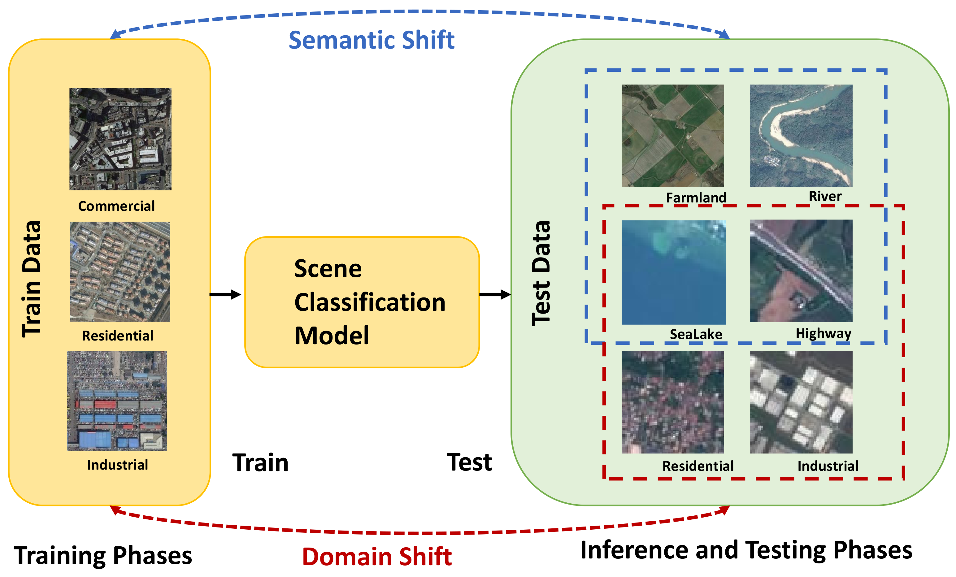
Supervised-learning-based remote sensing scene classification models are based on the closed-world assumption [11,12], that is, the test data are assumed to be independently and identically distributed to the training data [13], a situation referred to as in-distribution (ID). However, when the model is deployed in an open real-world scenario, the test data may be from a distribution different from that of the training dataset, referred to as out-of-distribution (OOD) [13]. For large-scale remote sensing scene classification tasks, it is common for the distributions of training and test sets to exhibit shifts [14]. Given the intricate nature of surface categories across diverse landscapes, model are prone to encountering semantic shifts during their application and deployment phases [13]. Additionally, domain shift [15,16] occurs in the distribution of remote sensing images collected across different datasets, owing to sensor differences and geographical disparities. We illustrate the concepts of semantic shift and domain shift in Figure 2. In these situations, the model tends to assign excessively high confidence levels, raising security concerns [17].
Over the past 5 years, numerous OOD detection methods have been proposed to ensure the safety and reliability of models [13]. The goal of OOD detection is to detect samples in which the model cannot be generalized [18]. Currently, the main OOD detection methods can be categorized as post hoc [19,20,21,22,23], training-time regulization [24,25], training with outlier exposure [26,27,28], and model uncertainty [29,30,31]. However, minimal attention has been given to OOD detection in remote sensing scene classification tasks. Previous research has focused on semantic shift due to the presence of new categories in the test set and addressed it using open-set-recognition (OSR) methods [32,33,34]. Al Rahhal et al. [35] proposed an end-to-end learning approach based on vision transformers and employed energy-based learning to jointly model the class labels and data distribution. Liu et al. [14] proposed a new loss function based on prototype learning and uncertainty measurement to enhance the interclass discrimination and intraclass compactness of the learned deep features. Gawlikowski et al. [16] developed a model based on a Dirichlet prior network to quantify the distributional uncertainty of deep-learning-based remote sensing models, utilizing this approach for OOD detection.
However, to the best of our knowledge, there is no unified benchmark for comparing and analyzing the effectiveness of various types of state-of-the-art OOD detection methods applied to remote sensing scene classification tasks, thereby leading to unfair comparisons and uncertain results. First, traditional evaluation benchmarks for OOD detection are not applicable to OOD detection of remote sensing imagery as these benchmarks are designed for general image datasets [36,37]. Nonetheless, remote sensing images from different datasets not only encounter semantic shifts but also face domain shifts due to variations in sensors and spatial distributions [38]. In addition, the performance of OOD detection methods vary widely across different datasets and benchmark comparisons [28,39]. Many simple comparison benchmarks for general image datasets are close to saturation, rendering improvements insignificant [18,40]. Therefore, it is crucial to design an out-of-distribution (OOD) detection benchmark and accurately assess the performance of existing methods on remote sensing datasets.
In this paper, we present the following key contributions:
- We establish benchmarks for evaluating OOD detection in remote sensing scene classification, using ResNet-50 as the backbone for all methods;
- We assess the effectiveness of various OOD detection methods across challenging datasets like AID, UCM, and EuroSAT, using metrics such as AUROC, FPR@95, and AUPR;
- We analyze performance disparities and challenges in applying these OOD detection methods to large-scale scene classification.
2. Methodology
In this section, we explore the concept of OOD and its related concepts and discuss the selected OOD detection methods and evaluation metrics. We prioritize using open-source code packages to quantitatively evaluate and compare their performance across different benchmarks. The selected methods align with the four most prominent research directions for OOD detection, as categorized in Table 1. Additionally, we present three benchmark remote sensing datasets and a backbone for scene classification and evaluate the performance of the models. Detailed implementation details are provided in the final part of this section.
2.1. Definition and Related Concepts
2.1.1. Definition
Remote sensing scene classification is a typical supervised multi-classification task [2,48]. For the remainder of this paper, we have assumed that represents the input space of the remote sensing images and represents the labeling space of the remote sensing images. Thus, the training data can be represented as , its distribution can be expressed as , and the marginal distribution can be denoted as . The process of a model trained on the training data is presented as , and the output of the model is denoted by the logit vector z, which is used to predict the output of the model.
We aim to deploy the model for remote sensing scene classification in the real world with a trustworthy OOD detector that not only accurately classifies data from the distribution (ID), but also recognizes data that do not belong to that distribution (OOD). The problem is expressed as a binary classification problem; that is, at the time of testing, the model must determine whether the input is from . This can be calculated using the following expression:
where represents the score of the sample, and samples with scores above a threshold are classified as ID; otherwise, they are classified as OOD. Scene classification models should not predict OOD samples, as no corresponding intersection in can be identified.
To better evaluate the performance of different models on remote sensing scene classification and examine the labels of OOD samples, we initially segmented the whole data space into four subspaces: , , , and . This division simplifies analysis by organizing samples into categories based on their connection to certain distributions. Each category shows a different level of uncertainty, from low to high. Our approach to segmenting the data and defining these categories draws from the methodology proposed by Liang et al. [19].
- (. Let X denote the input, . is a family of density functions on , is the parameter, denotes all the possible parameters that could generate samples in . represents the labeling space of the remote sensing images. Given a subset , we define ID data space as:
- (. We define Simi-OOD data space as:where .
- (. We define Near-OOD data space as:where
- . We define Far-OOD data space as:
For example, in UCM image sence classification, is the collection of all possible images and is UCM. If we consider each land cover category as a sample from a distribution, then is the collection of all the distributions with land use label as their expectations. Since UCM consists of 21 land cover categories, the density functions of UCM should be a subset of , that is, .
In the context of remote sensing scene classification with the UCM dataset, the consists of remote sensing images similar to UCM but with different styles. includes remote sensing images without UCM’s classes. comprises images unrelated to land cover or use. Labels for OOD data are inaccessible.
2.1.2. Related Concepts
The domains pertinent to Out-of-Distribution (OOD) detection encompass Open Set Recognition (OSR), Outlier Detection (OD), and One-Class Classification (OCC). A schematic representation delineating the conceptual distinctions among these domains is provided in Figure 3. We elucidate the specific differences between these concepts in the following.
- OOD detection vs. Open Set Recognition (OSR): In the context of remote sensing image scene classification tasks, OOD Detection and Open Set Recognition (OSR) share common ground, as both are concerned with identifying data points that deviate from the known distribution of training data. OSR focuses on distinguishing between known and unknown classes within classification problems, while OOD Detection involves a broader spectrum of learning tasks and extensive solution space;
- OOD detection vs. Outlier Detection (OD): In remote sensing outlier detection, a deviation from the conventional train–test paradigm occurs through the simultaneous presentation of all data, aligning with the framework of OOD detection by earmarking the principal data distribution as ID;
- OOD detection vs. One-Class Classification (OCC): In remote sensing one-class classification, normal or ID images are in one category; conversely, test images with semantic shift are classified as OOD, indicating they deviate from the norm.
2.2. Evaluating Methods
2.2.1. Post Hoc Methods
Post hoc methods do not require additional models and training data.These methods directly utilize the parameters in the original model to determine whether sample x is from . The advantages of this class of methods lie in their time efficiency and ease of use in practical production environments. For this class of methods, three widely used methods were selected for evaluation.
Maximum Softmax Probability (MSP) [17] is the simplest baseline method. This method detects OOD samples based on maximum softmax category probability.
The MSP method performs better when the difference between ID and OOD is large. However, when the difference between ID and OOD is small, this method may classify samples overconfidently owing to pretrained neural networks, which limits its detection performance.
Virtual-logit matching (VIM) [41] responds to diverse OOD samples by combining multiple inputs. The method first defines a virtual logit to generalize the common logit. The subspace S is set to be the orthogonal complementary space of the D-dimensional principal space P consisting of all training sample features. The larger the projection on , the more likely the sample is OOD.
The obtained is combined with other logits in softmax to obtain the final predicted probability for each class. corresponds to , which is the probability that the sample is OOD. Notate the set of orthogonal bases of as the matrix , the complete expression is as follows:
where is the matching coefficient.
This method demonstrates better overall performance on various types of datasets, does not require additional data for retraining, and offers a good degree of convenience.
Deep Nearest Neighbors (KNN) [42] utilizes a non-parametric nearest neighbor approach for OOD detection. It employs the normalized penultimate feature vector , where is a feature encoder. During testing, the normalized feature vector for a test sample is derived, and the Euclidean distances are calculated with respect to embedding vectors , where represents the embedding set of training data. The data sequence is reordered based on the increasing distance , denoted as . The decision function for OOD detection is defined as
The advantages of KNN-based OOD detection include distributional assumption-free testing, independence from unknown data information, user-friendly operation, and applicability to diverse model architectures.
2.2.2. Training-Time Regularization Methods
The training-time regularization class introduces additional setup conditions on top of the original model to solve the OOD detection problem using training-time regularization.
ConfBranch [43] incorporates an additional confidence branch to calculate confidence c and utilizes c as
The softmax prediction probability is adjusted using the confidence level c to obtain the new prediction probability .
Under this method, the model can effectively learn the decision boundaries of ID samples to obtain OOD detection.
Logit Normalization (LogitNorm) [44] was proposed to solve the problem of classifier overconfidence on OOD data. Specifically, the method limits the logit norm to a constant during the training process, while keeping the direction of the logit vector unchanged. The LogitNorm cross entropy can be expressed as:
This method does not require changes in the structure of the model and can be employed for OOD detection using metrics from a variety of post hoc methods. In this study, to ensure fair comparison, the maximum softmax probability value was computed via the benchmark method MSP to .
Generalized ODIN (G-ODIN) [45] defines the logits of category i as:
can be computed using the following formula, where is the feature of the penultimate layer, is the sigmoid function, BN denotes Batch Normalization, and w and b represent the learnable weights.
For , this can be realized by using a simple inner product (I):
The computational expression for is given by:
2.2.3. Training with Outlier Exposure Methods
This approach uses outliers for model training through an unsupervised approach. Outliers usually refer to the OOD data that can be collected. In this study, experiments with reference to these methods were performed using a Tiny-ImageNet dataset as outliers for model training.
Outlier Exposure (OE) [28] represents the baseline work for this branch. The method introduces a large-scale selected set of OODs as OEs and sets an additional training goal of expecting f to produce uniform softmax scores for the added data. Setting the original learning objective L, OE can be formalized as minimizing the objective:
This approach improves the generalization ability of the OOD detector, making it better suited for outlier distributions not observed previously. Additionally, this approach is suitable for models with different architectures.
Maximum Classifier Discrepancy (MCD) [27] utilizes a two-head deep convolutional neural network (CNN) and maximizes the discrepancy between classifiers and to detect OOD based on the discrepancy between the outputs of the two classifiers. and denote the K-dimensional softmax class probabilities for input x obtained by and , respectively. We used to measure the divergence between the two softmax class probabilities for an input. The discrepancy loss can be defined using the following equation:
where is the entropy over the softmax distribution. The experimental results of this method indicate that it has good generalization in real-world scenarios.
2.2.4. Model Uncertainty Methods
This approach allows the model to learn an attribute that is uncertain about the input samples. For the test data, the samples within a division exhibit low uncertainty, whereas those outside the distribution demonstrate high uncertainty. Model uncertainty methods primarily use Bayesian modeling to solve model reliability problems with less-principled approximations.
Monte Carlo Dropout (MCDropout) [46] predicts the same model and sample T times, and the variance of these T predictions is calculated to compute the uncertainty. Specifically, the method samples the posterior distribution of weights at test time using dropout to obtain the posterior distribution of softmax class probabilities. The means of these samples are used to segment the predictions and the variance is used to output the model uncertainty for each class. The probability of T sub-predictions can be expressed as:
where denotes the model parameters for each sample. The uncertainty can be measured using the following expression:
This method is easy to use and does not require modification of the existing neural network or additional training; it only requires the neural network to drop out.
TempScaling [47] learns and uses a temperature parameter T to calibrate the network. The calibrated predicted output is:
where denotes the softmax function, and when T tends to zero, the probability tends to , representing the maximum uncertainty. is the original softmax input. The parameter T is learned from the validation set using the NLL loss function. Temperature scaling does not affect the model accuracy.
TempScaling is one of the earliest and simplest methods for calibrating uncertainty measures; nevertheless, TempScaling is a variant of Platt Scaling, which is very effective in calibrating predictions.
2.3. Evaluating Metrics
OOD detection employs distinct evaluation metrics in contrast to conventional classification tasks [18]. Primarily, the distribution of categories in OOD detection typically exhibits an imbalance, characterized by fewer instances of unknown categories. Consequently, this imbalance predisposes models to favor known categories, thereby impacting accuracy metrics. Secondly, OOD detection places greater emphasis on the model’s false alarm rate, wherein the misclassification of unknown samples as known categories is a critical concern. Referring to Hendrycks’ metrics [17] and relevant assessments with reference to remote sensing [16,49], we used the following five metrics to quantitatively assess the effectiveness of the OOD detection method on the selected remote sensing datasets:
- Area Under the Receiver Operating Characteristic Curve (AUROC) is a common metric for evaluating the performance of a binary classification model, which represents the size of the area enclosed by the Receiver Operating Characteristic (ROC) curve and the axes, with a value range of 0–1. The ROC curve is plotted with False Positive Rate (FPR) as the horizontal axis and True Positive Rate (TPR) as the vertical axis, AUROC can be obtained by calculating the area enclosed under the ROC curve with the formula:
- Area Under the Precision–Recall Curve (AUPR) represents the size of the area enclosed by the Precision–Recall (PR) curve and the coordinate axes, and has values ranging from 0 to 1. AUPR can be obtained by calculating the area enclosed under the PR curve, and its formula is:
- False Positive Rate at 95% specificity (FPR@95) is the proportion of negative samples that are incorrectly predicted by the model when the model has a TPR of 95%. The formula for FPR@95 is as follows.where denotes the number of false positive classes (predicting negative classes as positive) and denotes the number of true negative classes (predicting negative classes as negative);
- ID classification accuracy (ID ACC) measures the overall correctness of predictions made by a model across all ID classes.The formula for ID ACC is as follows.where denotes false positives (predicting negative classes as positive) and denotes true negatives (predicting negative classes as negative). represents false negatives (misclassifying positive classes as negative), while represents true positives (correctly classifying negative classes as negative);
- Computation time, measured in seconds, is a key factor affecting the method’s practicality and is detailed in the paper.
2.4. Remote Sensing Datasets and Scene Classification Models
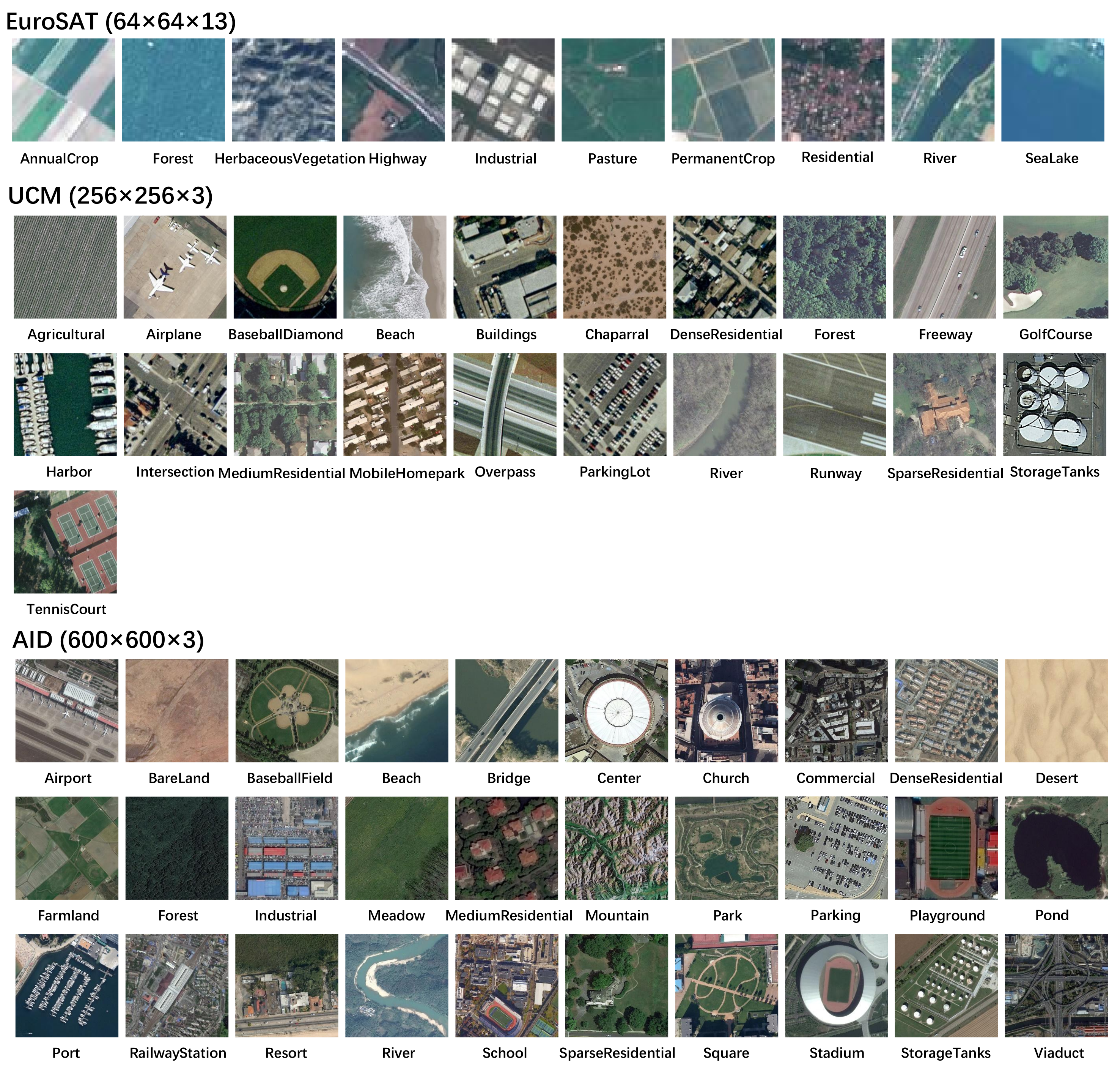
We conducted experiments on three different datasets: the Aerial Image dataset (AID), the UC-Merced Land Use (UCM) dataset, and Land Use and the Land Cover Classification with the Sentinel-2 (EuroSAR) dataset. We provide a brief description of these datasets below and the categories of the different datasets are shown in Figure 4.
- UCM Dataset: The UCM dataset [50] is a high-resolution aerial RGB image dataset. The size of each image is 256 × 256 pixels, and the dataset contains 21 categories with 100 samples in each category;
- AID Dataset: The AID dataset [51] is a high-resolution aerial RGB image dataset. The size of each image is 600 × 600 pixels, the dataset contains 30 categories, with each category containing 300 samples;
- EuroSAT Dataset: The EuroSAT Dataset [52] is a collection of images taken by the Sentinel-2 satellite, covering 13 spectral bands. Each image is 64 × 64 pixels in size, and the dataset consists of 10 categories, each containing 2000 to 3000 images, totaling 27,000 samples.
In the field of scene classification, numerous models have been developed for the UCM, AID, and EuroSAT datasets. Among these, Resnet [53] has achieved state-of-the-art results on all three datasets [2]. Based on Table 2, ResNet-50 has relatively fewer parameters, requires lower FLOPS, and has a shorter training time. Considering both performance and efficiency, this study selects ResNet-50 as the backbone for all the tested Out-of-Distribution (OOD) detection models.
2.5. Implementation Details and Parameter Selection
To compare different methods from different domains fairly, we used a unified setup and hyperparameter architecture. For the remote sensing scene classification models, we uniformly used ResNet-50 as the benchmark. If the implemented method required training, we used the accepted settings of the SGD optimizer with a learning rate of 0.01, momentum of 0.9, and weight decay of 0.0005 for 100 epochs to prevent over-tuning. If the method requires hyperparameter tuning, we explored only the five most common values and selected hyperparameters based on the performance of AUROC on the validation set. The logic of the OOD validation set selection is based on real-world practices, all of which are designed for fairness and utility in comparison with benchmarks. The main benchmark development and testing were conducted using four Nvidia RTX 2080Ti cards.
2.6. Benchmarks
To test the performance of different OOD detection methods under semantic shift and domain shift, we referred to the construction of OOD detection benchmarks for general images, designed a series of benchmarks on AID, UCM, and EuroSAT datasets by combining the characteristics of remote sensing images themselves, and conducted many experiments. Our benchmarks can be categorized into OSR benchmarks and OOD benchmarks. Refer to Figure 5 for a diagram illustrating these benchmarks.
2.6.1. OSR Benchmarks
In developing benchmarks for evaluating Open-Set-Recognition (OSR) performance, we drew inspiration from established benchmarks such as MNIST [61] and CIFAR [62]. These benchmarks typically use different class divisions, for example, 6/4 and 50/50, to test models’ abilities to identify instances of open set samples within the test set. To implement this, we divided dataset categories into two groups: closed and open sets. Models are then trained exclusively on data from the closed set and are evaluated on the entire test set to ascertain their proficiency in distinguishing between closed and open set samples.
For datasets like AID, UCM, and EuroSAT, we introduced specific configurations—namely AID7/3, AID6/4, AID5/5, UCM7/3, UCM6/4, UCM5/5, and EuroSAT 7/3, EuroSAT 6/4, EuroSAT 5/5. These configurations indicate the ratio of closed-set to open-set classes, such as 7:3, 6:4, and 5:5, respectively. A detailed methodology for one of these randomized divisions is presented in Table 3, illustrating our approach.
The benchmarks we developed are based on randomized class divisions. The performance metrics we utilize are derived from the average outcomes of five distinct splits, ensuring a comprehensive assessment of a model’s ability to handle open set samples. This methodology ensures that our benchmarks effectively measure a model’s OSR performance, contributing valuable insights into their capabilities in dealing with open set scenarios.
2.6.2. OOD Benchmarks
The common practice for building OOD detection benchmarks is to consider an entire dataset as in-distribution (ID), and then collect several datasets that are disconnected from any ID categories as OOD datasets [17]. To better evaluate the model under semantic and domain shifts, according to the definitions of , , and , we have designed a total of nine out-of-distribution (OOD) benchmarks across three datasets: UCM, AID, and EuroSAT. These benchmarks are named using the dataset name followed by the definition of the distribution. Specifically, these benchmarks are UCM-Simi-OOD, UCM-Near-OOD, UCM-Far-OOD, AID-Simi-OOD, AID-Near-OOD, AID-Far-OOD, EuroSAT-Simi-OOD, EuroSAT-Near-OOD, and EuroSAT-Far-OOD. We provide detailed descriptions of these nine benchmarks below. In Table 4, we present the specific categorization of the Simi-OOD and Near-OOD classes across different datasets.
- In the Simi-OOD benchmark for the UCM dataset, we incorporated 20 categories exhibiting semantic overlap with RSI-CB256 [63] and UCM [50]. Conversely, the Near-OOD subset featured an additional 15 categories that do not intersect with this overlap. Our Far-OOD compilation encompasses datasets such as Places365 [64], ImageNet-O [65], and OpenImage-O [41], which we resized to to align with our Far-OOD criterion;
- In the Simi-OOD benchmark for the AID dataset, we focused on 20 categories sharing semantic traits between NWPU-RESISC45 [2] and AID [51]. In contrast, the Near-OOD category embraced an additional 15 categories with no overlap. To address Far-OOD scenarios, we integrated datasets like Places365 [64], ImageNet-O [65], and OpenImage-O [41], resizing images to to match our definitions of Simi-OOD, Near-OOD and Far-OOD;
- In the EuroSAT dataset within the Simi-OOD benchmark, we examined 10 categories sharing semantic features between RSI-CB128 [63] and EuroSAT [52]. Conversely, the Near-OOD subset encompassed an additional 35 categories devoid of overlap. Our Far-OOD consideration included datasets like MNIST [61], CIFAR-100 [62], and Tiny-Imagenet [12]. Resizing images to aligned with our definitions of Near-OOD and Far-OOD.
3. Results
3.1. Results on OSR Benchmark
The methods we tested rely on a ResNet-50 backbone trained on closed-set data corresponding to UCM, AID, and EuroSAT. To quantify the reliability of the OOD detection model, we used AUROC, FPR@95, AUPR-IN, and AUPR-OUT metrics. In addition, the computation time, as an aspect of the applicability of the methods, was evaluated and recorded in seconds. For the AUROC score, AUPR-IN, and AUPR-OUT score, higher scores were considered better, and for the FPR@95 score and computation time metric, lower scores were considered better.
According to Table 5, the VIM and KNN methods, which require no additional training, achieved the best results in AUROC, ranking in the top three across different OSR-AID and OSR-UCM benchmark splits. Table 6 reveals that, in addition to VIM and KNN, the LogiNorm method also secured a top-three position in FPR@95 across different benchmarks, achieving the lowest values in some benchmarks. As per Table 7 and Table 8, the OE method, alongside VIM and KNN, performed well in the AUPR-IN and AUPR-OUT metrics. According to Table 9, all evaluated methods scored highly on the ID ACC metric. Table 10 indicates that methods such as MSP, VIM, and KNN, which do not require additional training time, had the shortest computation times, making them more suitable for scenarios with high real-time requirements.
Overall, the VIM and KNN methods demonstrated excellent performance across all evaluation metrics without the need for additional training. Surprisingly, methods requiring substantial additional training time, such as OE and MCD, did not achieve better AUROC values, suggesting that additional training processes are unnecessary for the OSR benchmarks. The performance of ConfBranch and G-ODIN methods was suboptimal across all OSR benchmarks. An analysis of Table 5 shows that ConfBranch had higher AUROC values on the EuroSAT benchmark than on the AID benchmark, and even more so compared to the UCM dataset, indicating a propensity for overfitting on smaller-scale datasets (e.g., UCM) and suggesting its better suitability for larger datasets. The performance of the G-ODIN method, which requires an additional training process, was inferior to other methods, indicating the need for finer parameter tuning when applied to remote sensing imagery, such as exploring different distance functions .
Furthermore, results from Figure 6 illustrate that nearly all methods performed better on the 7/3 split for AUROC and AUPR metrics compared to the 6/4 split, and significantly better than the 5/5 split. This can likely be attributed to the openness of the different benchmarks, with the 5/5 split having the highest openness and thus presenting a greater challenge. Additionally, the analysis of the AUPR-IN and AUPR-OUT results indicates an inverse effect of category division on these metrics. The 5/5 split showed better performance in AUPR-IN compared to other splits, while its performance in AUPR-OUT was poorer, likely due to the higher probability of similar features being classified as in-distribution or out-of-distribution, leading to higher AUPR-IN and lower AUPR-OUT.
3.2. Results on OOD Benchmark
The methods we tested rely on a ResNet-50 backbone network trained on the entire UCM, AID, and EuroSAT datasets. Figure 7 illustrates the test results on the OOD benchmark, showing the AUROC, FPR@95, AUPR-IN, and AUPR-OUT metrics of 10 methods primarily on the OOD benchmark. Moreover, more detailed results are provided in Table 11, Table 12, Table 13 and Table 14. In addition to the previously mentioned metrics, the in-distribution accuracy (ID-ACC) and overall computation time are also presented in Table 15 and Table 16, respectively.
Overall, among all performance metrics, the VIM method without additional training and the OE method requiring extra training and auxiliary data achieve high AUROC values and low [email protected], the ConfBranch and G-ODIN methods exhibit below-average performance across all OOD benchmarks, indicating limited applicability in OOD benchmarking. Surprisingly, the KNN method, which performs well on the OSR benchmark, demonstrates poor performance on our UCM and AID benchmarks of OOD. Specifically, the AUPR-OUT scores are notably low on UCM and AID, indicating poor classification of out-of-distribution data. This result might arise from the unequal sample sizes between out-of-distribution and in-distribution data, necessitating further fine-tuning of hyperparameters, particularly K, to align with our OOD benchmarks.
Additionally, based on Figure 7, it is observed that nearly all methods demonstrate better performance in AUROC and AUPR metrics on Far-OOD compared to Near-OOD, which in turn outperforms Simi-OOD. This suggests that the Simi-OOD benchmarks, which identify domain shift exclusively, pose the greatest challenge. Conversely, simultaneously detecting both domain shift and semantic shift in Near-OOD benchmarks is relatively easier, while Far-OOD benchmarks, characterized by significantly greater semantic shift, are the most manageable. In AUPR-IN, different methods generally perform better on Near-OOD benchmarks. However, in AUPR-OUT, Far-OOD benchmarks exhibit superior performance overall. This indicates that models find it relatively more challenging to discern remote sensing image datasets compared to conventional image datasets, consistent with our expectations.
4. Discussion
Based on our research findings, we have discovered that existing methods for detecting out-of-distribution (OOD) instances are quite applicable to remote sensing scene classification tasks. However, the current research is predominantly based on common datasets, and there is a notable gap when it comes to applying these methods to real-world remote sensing scene classifications. Firstly, the semantic clarity under different scenes in remote sensing scene classification tasks is lacking, with insufficiently pronounced differences between classes, necessitating the detection of certain features at a finer granularity. Additionally, significant variance exists within the same category, and identical feature types can vary extensively due to time, geographical location, and spatial scale. Moreover, due to the resolution of images used in real-world scenarios and the substantial variance in the spectral reflectance of images, identifying sensor shifts caused by different sensors is a topic worth investigating.
To enhance the reliability of remote sensing scene classification models in open scenarios, we believe further exploration in the following directions could improve the performance of OOD detection models. Firstly, this research has validated the effectiveness of post hoc methods, which do not require an additional training process. Therefore, these methods can be further explored in real-world scenarios. Secondly, in real-world scene classification tasks, it is sometimes necessary to differentiate between in-distribution (ID) and OOD instances within a small range, such as distinguishing between airports and roads [66]. Hence, fine-grained features could be further extracted from a fine-grained classification perspective for OOD detection. Lastly, due to the semantic ambiguity in single-label classification of remote sensing samples [67], we believe that developing OOD detection methods suited for multi-label classification will be useful for large-scale remote sensing scene classification tasks.
5. Conclusions
We evaluated different classes of OOD detection methods that are highly representative of the corresponding research directions to improve the reliability and security of remote sensing scene classification models. To further compare the performances of the different methods under semantic and domain shifts, we set up a series of benchmarks on the AID, UCM, and EuroSAT datasets. We quantitatively evaluated them using AUROC, AUPR, FPR@95, ID-ACC, and computation time metrics. We conducted numerous experiments to quantitatively evaluate the performance of these methods across different benchmarks. Based on the evaluation results, we found that that virtual-logit matching methods, without extra training, perform better than other methods on both OSR and OOD benchmarks. This suggests that additional training methods are unnecessary for scene classification applications in remote sensing imagery. Our results show that existing OOD detection methods can provide reliability and security for further deployment of remote sensing scene categorization applications with large-scale, diverse ground coverage involving multiple types of sensors. Additionally, our findings provide valuable insights to explore better OOD detection methods suitable for large-scale remote sensing applications.
Author Contributions
Conceptualization, S.L.; methodology, S.L.; software, S.L.; validation, S.L. and N.L.; formal analysis, S.L.; investigation, S.L.; resources, S.L. and M.J.; data curation, S.L.; writing— original draft preparation, S.L.; writing—review and editing, C.J.; visualization, S.L. and N.L.; supervision, C.J.; project administration, L.C.; funding acquisition, L.C. All authors have read and agreed to the published version of the manuscript.
Funding
This research was funded by the Foundation of Science & Technology on Integrated Information System Laboratory (HLJGXQ20220916032) and by the National Key Research and Development Program of China (2022YFB3903603).
Data Availability Statement
Data associated with this research are available online. The UCM dataset is available at http://weegee.vision.ucmerced.edu/datasets/landuse.html (accessed on 5 March 2024). The AID datasets are available at https://opendatalab.com/OpenDataLab/AID (accessed on 5 March 2024). The EuroSAT dataset is available at https://opendatalab.com/OpenDataLab/EuroSAT (accessed on 5 March 2024).
Conflicts of Interest
The authors declare no conflicts of interest.
References
- Ma, L.; Liu, Y.; Zhang, X.; Ye, Y.; Yin, G.; Johnson, B.A. Deep learning in remote sensing applications: A meta-analysis and review. ISPRS J. Photogramm. Remote Sens. 2019, 152, 166–177. [Google Scholar] [CrossRef]
- Cheng, G.; Han, J.; Lu, X. Remote sensing image scene classification: Benchmark and state of the art. Proc. IEEE 2017, 105, 1865–1883. [Google Scholar] [CrossRef]
- Nogueira, K.; Penatti, O.A.; Dos Santos, J.A. Towards better exploiting convolutional neural networks for remote sensing scene classification. Pattern Recognit. 2017, 61, 539–556. [Google Scholar] [CrossRef]
- Bouslihim, Y.; Kharrou, M.H.; Miftah, A.; Attou, T.; Bouchaou, L.; Chehbouni, A. Comparing pan-sharpened Landsat-9 and Sentinel-2 for land-use classification using machine learning classifiers. J. Geovis. Spat. Anal. 2022, 6, 35. [Google Scholar] [CrossRef]
- Dimitrovski, I.; Kitanovski, I.; Kocev, D.; Simidjievski, N. Current trends in deep learning for Earth Observation: An open-source benchmark arena for image classification. ISPRS J. Photogramm. Remote Sens. 2023, 197, 18–35. [Google Scholar] [CrossRef]
- Vernekar, S.; Gaurav, A.; Denouden, T.; Phan, B.; Abdelzad, V.; Salay, R.; Czarnecki, K. Analysis of confident-classifiers for out-of-distribution detection. arXiv 2019, arXiv:1904.12220. [Google Scholar]
- Tang, K.; Miao, D.; Peng, W.; Wu, J.; Shi, Y.; Gu, Z.; Tian, Z.; Wang, W. Codes: Chamfer out-of-distribution examples against overconfidence issue. In Proceedings of the IEEE/CVF International Conference on Computer Vision, Montreal, QC, Canada, 10–17 October 2021; pp. 1153–1162. [Google Scholar]
- Berger, C.; Paschali, M.; Glocker, B.; Kamnitsas, K. Confidence-based out-of-distribution detection: A comparative study and analysis. In Proceedings of the Uncertainty for Safe Utilization of Machine Learning in Medical Imaging, and Perinatal Imaging, Placental and Preterm Image Analysis: 3rd International Workshop, UNSURE 2021, and 6th International Workshop, PIPPI 2021, Held in Conjunction with MICCAI 2021, Strasbourg, France, 1 October 2021; Proceedings 3. Springer: Berlin/Heidelberg, Germany, 2021; pp. 122–132. [Google Scholar]
- Hendrycks, D.; Carlini, N.; Schulman, J.; Steinhardt, J. Unsolved problems in ml safety. arXiv 2021, arXiv:2109.13916. [Google Scholar]
- Hendrycks, D.; Mazeika, M. X-risk analysis for ai research. arXiv 2022, arXiv:2206.05862. [Google Scholar]
- He, K.; Zhang, X.; Ren, S.; Sun, J. Delving deep into rectifiers: Surpassing human-level performance on imagenet classification. In Proceedings of the IEEE International Conference on Computer Vision, Santiago, Chile, 11–18 December 2015; pp. 1026–1034. [Google Scholar]
- Krizhevsky, A.; Sutskever, I.; Hinton, G.E. Imagenet classification with deep convolutional neural networks. Adv. Neural Inf. Process. Syst. 2012, 60, 84–90. [Google Scholar] [CrossRef]
- Yang, J.; Zhou, K.; Li, Y.; Liu, Z. Generalized out-of-distribution detection: A survey. arXiv 2021, arXiv:2110.11334. [Google Scholar]
- Liu, W.; Nie, X.; Zhang, B.; Sun, X. Incremental Learning With Open-Set Recognition for Remote Sensing Image Scene Classification. IEEE Trans. Geosci. Remote Sens. 2022, 60, 1–16. [Google Scholar] [CrossRef]
- Zhou, K.; Liu, Z.; Qiao, Y.; Xiang, T.; Loy, C.C. Domain generalization: A survey. IEEE Trans. Pattern Anal. Mach. Intell. 2022, 45, 4396–4415. [Google Scholar] [CrossRef] [PubMed]
- Gawlikowski, J.; Saha, S.; Kruspe, A.; Zhu, X.X. An advanced dirichlet prior network for out-of-distribution detection in remote sensing. IEEE Trans. Geosci. Remote Sens. 2022, 60, 1–19. [Google Scholar] [CrossRef]
- Hendrycks, D.; Gimpel, K. A baseline for detecting misclassified and out-of-distribution examples in neural networks. arXiv 2016, arXiv:1610.02136. [Google Scholar]
- Yang, J.; Wang, P.; Zou, D.; Zhou, Z.; Ding, K.; Peng, W.; Wang, H.; Chen, G.; Li, B.; Sun, Y.; et al. Openood: Benchmarking generalized out-of-distribution detection. Adv. Neural Inf. Process. Syst. 2022, 35, 32598–32611. [Google Scholar]
- Liang, S.; Li, Y.; Srikant, R. Enhancing the reliability of out-of-distribution image detection in neural networks. arXiv 2017, arXiv:1706.02690. [Google Scholar]
- Lee, K.; Lee, K.; Lee, H.; Shin, J. A simple unified framework for detecting out-of-distribution samples and adversarial attacks. Adv. Neural Inf. Process. Syst. 2018, 31. [Google Scholar]
- Liu, W.; Wang, X.; Owens, J.; Li, Y. Energy-based out-of-distribution detection. Adv. Neural Inf. Process. Syst. 2020, 33, 21464–21475. [Google Scholar]
- Sastry, C.S.; Oore, S. Detecting out-of-distribution examples with gram matrices. In Proceedings of the International Conference on Machine Learning. PMLR, Virtual, 13–18 July 2020; pp. 8491–8501. [Google Scholar]
- Sun, Y.; Li, Y. Dice: Leveraging sparsification for out-of-distribution detection. In Proceedings of the European Conference on Computer Vision, Tel Aviv, Israel, 23–27 October 2022; Springer: Berlin/Heidelberg, Germany, 2022; pp. 691–708. [Google Scholar]
- Du, X.; Wang, Z.; Cai, M.; Li, Y. Vos: Learning what you do not know by virtual outlier synthesis. arXiv 2022, arXiv:2202.01197. [Google Scholar]
- Tack, J.; Mo, S.; Jeong, J.; Shin, J. Csi: Novelty detection via contrastive learning on distributionally shifted instances. Adv. Neural Inf. Process. Syst. 2020, 33, 11839–11852. [Google Scholar]
- Yang, J.; Wang, H.; Feng, L.; Yan, X.; Zheng, H.; Zhang, W.; Liu, Z. Semantically coherent out-of-distribution detection. In Proceedings of the IEEE/CVF International Conference on Computer Vision, Montreal, BC, Canada, 11–17 October 2021; pp. 8301–8309. [Google Scholar]
- Yu, Q.; Aizawa, K. Unsupervised out-of-distribution detection by maximum classifier discrepancy. In Proceedings of the IEEE/CVF International Conference on Computer Vision, Seoul, Republic of Korea, 27 October–2 November 2019; pp. 9518–9526. [Google Scholar]
- Hendrycks, D.; Mazeika, M.; Dietterich, T. Deep anomaly detection with outlier exposure. arXiv 2018, arXiv:1812.04606. [Google Scholar]
- Lakshminarayanan, B.; Pritzel, A.; Blundell, C. Simple and scalable predictive uncertainty estimation using deep ensembles. Adv. Neural Inf. Process. Syst. 2017, 30. [Google Scholar]
- Scheirer, W.J.; Jain, L.P.; Boult, T.E. Probability models for open set recognition. IEEE Trans. Pattern Anal. Mach. Intell. 2014, 36, 2317–2324. [Google Scholar] [CrossRef] [PubMed]
- Smith, R. Extreme value theory. In Handbook of Applicable Mathematics; Wiley: Hoboken, NJ, USA, 1990; Volume 7. [Google Scholar]
- Ge, Z.; Demyanov, S.; Chen, Z.; Garnavi, R. Generative openmax for multi-class open set classification. arXiv 2017, arXiv:1707.07418. [Google Scholar]
- Neal, L.; Olson, M.; Fern, X.; Wong, W.K.; Li, F. Open set learning with counterfactual images. In Proceedings of the European Conference on Computer Vision (ECCV), Munich, Germany, 8–14 September 2018; pp. 613–628. [Google Scholar]
- Scheirer, W.J.; de Rezende Rocha, A.; Sapkota, A.; Boult, T.E. Toward open set recognition. IEEE Trans. Pattern Anal. Mach. Intell. 2012, 35, 1757–1772. [Google Scholar] [CrossRef]
- Al Rahhal, M.M.; Bazi, Y.; Al-Dayil, R.; Alwadei, B.M.; Ammour, N.; Alajlan, N. Energy-based learning for open-set classification in remote sensing imagery. Int. J. Remote Sens. 2022, 43, 6027–6037. [Google Scholar] [CrossRef]
- Li, C.L.; Sohn, K.; Yoon, J.; Pfister, T. Cutpaste: Self-supervised learning for anomaly detection and localization. In Proceedings of the IEEE/CVF Conference on Computer Vision and Pattern Recognition, Nashville, TN, USA, 20–25 June 2021; pp. 9664–9674. [Google Scholar]
- Hein, M.; Andriushchenko, M.; Bitterwolf, J. Why relu networks yield high-confidence predictions far away from the training data and how to mitigate the problem. In Proceedings of the IEEE/CVF Conference on Computer Vision and Pattern Recognition, Long Beach, CA, USA, 15–20 June 2019; pp. 41–50. [Google Scholar]
- da Silva, C.C.; Nogueira, K.; Oliveira, H.N.; dos Santos, J.A. Towards open-set semantic segmentation of aerial images. In Proceedings of the 2020 IEEE Latin American GRSS & ISPRS Remote Sensing Conference (LAGIRS), Santiago, Chile, 22–26 March 2020; pp. 16–21. [Google Scholar]
- Torralba, A.; Fergus, R.; Freeman, W.T. 80 million tiny images: A large data set for nonparametric object and scene recognition. IEEE Trans. Pattern Anal. Mach. Intell. 2008, 30, 1958–1970. [Google Scholar] [CrossRef] [PubMed]
- Zou, Y.; Yu, Z.; Liu, X.; Kumar, B.; Wang, J. Confidence regularized self-training. In Proceedings of the IEEE/CVF International Conference on Computer Vision, Seoul, Republic of Korea, 27 October–2 November 2019; pp. 5982–5991. [Google Scholar]
- Wang, H.; Li, Z.; Feng, L.; Zhang, W. Vim: Out-of-distribution with virtual-logit matching. In Proceedings of the IEEE/CVF Conference on Computer Vision and Pattern Recognition, New Orleans, LA, USA, 18–24 June 2022; pp. 4921–4930. [Google Scholar]
- Sun, Y.; Ming, Y.; Zhu, X.; Li, Y. Out-of-distribution detection with deep nearest neighbors. In Proceedings of the International Conference on Machine Learning, PMLR, Baltimore, MD, USA, 17–23 July 2022; pp. 20827–20840. [Google Scholar]
- DeVries, T.; Taylor, G.W. Learning confidence for out-of-distribution detection in neural networks. arXiv 2018, arXiv:1802.04865. [Google Scholar]
- Wei, H.; Xie, R.; Cheng, H.; Feng, L.; An, B.; Li, Y. Mitigating neural network overconfidence with logit normalization. In Proceedings of the International Conference on Machine Learning, PMLR, Baltimore, MD, USA, 25–27 July 2022; pp. 23631–23644. [Google Scholar]
- Hsu, Y.C.; Shen, Y.; Jin, H.; Kira, Z. Generalized odin: Detecting out-of-distribution image without learning from out-of-distribution data. In Proceedings of the IEEE/CVF Conference on Computer Vision and Pattern Recognition, Seattle, WA, USA, 13–19 June 2020; pp. 10951–10960. [Google Scholar]
- Gal, Y.; Ghahramani, Z. Dropout as a bayesian approximation: Representing model uncertainty in deep learning. In Proceedings of the International Conference on Machine Learning, PMLR, New York, NY, USA, 19–24 June 2016; pp. 1050–1059. [Google Scholar]
- Guo, C.; Pleiss, G.; Sun, Y.; Weinberger, K.Q. On calibration of modern neural networks. In Proceedings of the International Conference on Machine Learning, PMLR, Sydney, Australia, 6–11 August 2017; pp. 1321–1330. [Google Scholar]
- Faqe Ibrahim, G.R.; Rasul, A.; Abdullah, H. Improving crop classification accuracy with integrated Sentinel-1 and Sentinel-2 data: A case study of barley and wheat. J. Geovis. Spat. Anal. 2023, 7, 22. [Google Scholar] [CrossRef]
- He, Y.; Zhao, Z.; Zhu, Q.; Liu, T.; Zhang, Q.; Yang, W.; Zhang, L.; Wang, Q. An integrated neural network method for landslide susceptibility assessment based on time-series InSAR deformation dynamic features. Int. J. Digit. Earth 2024, 17, 2295408. [Google Scholar] [CrossRef]
- Yang, Y.; Newsam, S. Bag-of-visual-words and spatial extensions for land-use classification. In Proceedings of the 18th SIGSPATIAL International Conference on Advances in Geographic Information Systems, San Jose, CA, USA, 2–5 November 2010; pp. 270–279. [Google Scholar]
- Xia, G.S.; Hu, J.; Hu, F.; Shi, B.; Bai, X.; Zhong, Y.; Zhang, L.; Lu, X. AID: A benchmark data set for performance evaluation of aerial scene classification. IEEE Trans. Geosci. Remote Sens. 2017, 55, 3965–3981. [Google Scholar] [CrossRef]
- Helber, P.; Bischke, B.; Dengel, A.; Borth, D. Eurosat: A novel dataset and deep learning benchmark for land use and land cover classification. IEEE J. Sel. Top. Appl. Earth Obs. Remote Sens. 2019, 12, 2217–2226. [Google Scholar] [CrossRef]
- He, K.; Zhang, X.; Ren, S.; Sun, J. Deep residual learning for image recognition. In Proceedings of the IEEE Conference on Computer Vision and Pattern Recognition, Las Vegas, NV, USA, 26 June–1 July 2016; pp. 770–778. [Google Scholar]
- Simonyan, K.; Zisserman, A. Very deep convolutional networks for large-scale image recognition. arXiv 2014, arXiv:1409.1556. [Google Scholar]
- Huang, G.; Liu, Z.; Van Der Maaten, L.; Weinberger, K.Q. Densely connected convolutional networks. In Proceedings of the IEEE Conference on Computer Vision and Pattern Recognition, Honolulu, HI, USA, 21–26 July 2017; pp. 4700–4708. [Google Scholar]
- Tan, M.; Le, Q. Efficientnet: Rethinking model scaling for convolutional neural networks. In Proceedings of the International Conference on Machine Learning, PMLR, Long Beach, CA, USA, 9–15 June 2019; pp. 6105–6114. [Google Scholar]
- Dosovitskiy, A.; Beyer, L.; Kolesnikov, A.; Weissenborn, D.; Zhai, X.; Unterthiner, T.; Dehghani, M.; Minderer, M.; Heigold, G.; Gelly, S.; et al. An image is worth 16x16 words: Transformers for image recognition at scale. arXiv 2020, arXiv:2010.11929. [Google Scholar]
- Tolstikhin, I.O.; Houlsby, N.; Kolesnikov, A.; Beyer, L.; Zhai, X.; Unterthiner, T.; Yung, J.; Steiner, A.; Keysers, D.; Uszkoreit, J.; et al. Mlp-mixer: An all-mlp architecture for vision. Adv. Neural Inf. Process. Syst. 2021, 34, 24261–24272. [Google Scholar]
- Liu, Z.; Mao, H.; Wu, C.Y.; Feichtenhofer, C.; Darrell, T.; Xie, S. A convnet for the 2020s. In Proceedings of the IEEE/CVF Conference on Computer Vision and Pattern Recognition, New Orleans, LA, USA, 18–24 June 2022; pp. 11976–11986. [Google Scholar]
- Liu, Z.; Hu, H.; Lin, Y.; Yao, Z.; Xie, Z.; Wei, Y.; Ning, J.; Cao, Y.; Zhang, Z.; Dong, L.; et al. Swin transformer v2: Scaling up capacity and resolution. In Proceedings of the IEEE/CVF Conference on Computer Vision and Pattern Recognition, New Orleans, LA, USA, 18–24 June 2022; pp. 12009–12019. [Google Scholar]
- Mu, N.; Gilmer, J. MNIST-C: A Robustness Benchmark for Computer Vision. arXiv, 2019; arXiv:1906.02337. [Google Scholar]
- Krizhevsky, A.; Hinton, G.; Sutskever, I.; Salakhutdinov, R.; Osindero, S.; Teh, Y.W.; Tieleman, T.; Mnih, A.; Hadsell, R.; Eslami, S.M.A.; et al. Learning Multiple Layers of Features from Tiny Images; Technical Report; University of Toronto: Toronto, ON, Canada, 2009; pp. 32–33. [Google Scholar]
- Li, H.; Dou, X.; Tao, C.; Wu, Z.; Chen, J.; Peng, J.; Deng, M.; Zhao, L. RSI-CB: A large-scale remote sensing image classification benchmark using crowdsourced data. Sensors 2020, 20, 1594. [Google Scholar] [CrossRef] [PubMed]
- Zhou, B.; Lapedriza, A.; Khosla, A.; Oliva, A.; Torralba, A. Places: A 10 million image database for scene recognition. IEEE Trans. Pattern Anal. Mach. Intell. 2017, 40, 1452–1464. [Google Scholar] [CrossRef] [PubMed]
- Hendrycks, D.; Zhao, K.; Basart, S.; Steinhardt, J.; Song, D. Natural adversarial examples. In Proceedings of the IEEE/CVF Conference on Computer Vision and Pattern Recognition, Nashville, TN, USA, 20–25 June 2021; pp. 15262–15271. [Google Scholar]
- Li, N.; Cheng, L.; Ji, C.; Dongye, S.; Li, M. An Improved Framework for Airport Detection Under the Complex and Wide Background. IEEE J. Sel. Top. Appl. Earth Obs. Remote Sens. 2022, 15, 9545–9555. [Google Scholar] [CrossRef]
- Shao, Z.; Yang, K.; Zhou, W. Performance evaluation of single-label and multi-label remote sensing image retrieval using a dense labeling dataset. Remote Sens. 2018, 10, 964. [Google Scholar] [CrossRef]
Figure 1.
A remote sensing scene classification model trained on a closed dataset tends to encounter challenges when faced with unknown categories in open-world scenarios. In such cases, the model often categorizes them as known ones.
Figure 1.
A remote sensing scene classification model trained on a closed dataset tends to encounter challenges when faced with unknown categories in open-world scenarios. In such cases, the model often categorizes them as known ones.

Figure 2.
When deploying a remote sensing scene classification model in the real world, challenges arise during inference and testing. These challenges include images with land cover categories not found in the training dataset (referred to as semantic shift) or images with the same categories but differing sensor differences and geographical disparities (referred to as domain shift). Models often tend to classify such images as known categories.

Figure 3.
Conception of One-Class Classification, Open Set Recognition, Out-of-Distribution Detection and Outlier Detection.
Figure 3.
Conception of One-Class Classification, Open Set Recognition, Out-of-Distribution Detection and Outlier Detection.

Figure 4.
Classes and corresponding examples for the EuroSAT dataset, the UCM dataset, and the AID dataset. For the EuroSAT dataset, only images consisting of the three bands red, green, and blue are shown.
Figure 4.
Classes and corresponding examples for the EuroSAT dataset, the UCM dataset, and the AID dataset. For the EuroSAT dataset, only images consisting of the three bands red, green, and blue are shown.

Figure 5.
We established nine OSR benchmarks and nine OOD benchmarks on the UCM, AID, and EuroSAT datasets. Among them, OSR benchmarks only detect semantic shifts, while OOD benchmarks further detect domain shifts.
Figure 5.
We established nine OSR benchmarks and nine OOD benchmarks on the UCM, AID, and EuroSAT datasets. Among them, OSR benchmarks only detect semantic shifts, while OOD benchmarks further detect domain shifts.

Figure 6.
Performance against OSR Benchmark.

Figure 7.
Performance against OOD benchmark.


Table 1.
List of different types of OOD detection methods for remote sensing scene classification tasks.
Table 1.
List of different types of OOD detection methods for remote sensing scene classification tasks.
| Methodology | Reference | ||
| OOD detection methods | post hoc | MSP | [17] |
| VIM | [41] | ||
| KNN | [42] | ||
| training-time regularization | ConfBranch | [43] | |
| LogitNorm | [44] | ||
| G-ODIN | [45] | ||
| training with outlier exposure | OE | [28] | |
| MCD | [27] | ||
| model uncertainty | MCDropout | [46] | |
| Tempscaling | [47] | ||
Table 2.
Summary of recent representative model architectures.
| Model | Year | Layers | Parameters | FLOPS | Reference |
|---|---|---|---|---|---|
| AlexNet | 2012 | 8 | ∼ | 0.72 G | [12] |
| VGG16 | 2014 | 16 | ∼ | 15.47 G | [54] |
| ResNet50 | 2015 | 50 | ∼ | 4.09 G | [53] |
| ResNet152 | 2015 | 152 | ∼ | 11.52 G | [53] |
| DenseNet161 | 2017 | 161 | ∼ | 7.73 G | [55] |
| EfficientNet B0 | 2019 | 237 | ∼ | 0.39 G | [56] |
| Vision Transformer | 2020 | 12 | ∼ | 17.57 G | [57] |
| MLPMixer | 2021 | 12 | ∼ | 12.61 G | [58] |
| ConvNeXt | 2022 | 174 | ∼ | 4.46 G | [59] |
| Swin Transformer | 2022 | 24 | ∼ | 11.55 G | [60] |
Table 3.
The 30 classes in AID, the 21 classes in UCM, and the 10 classes in EuroSAT were divided into closed-set and open-set classes according to defined proportions in various benchmarks. Five randomizations were conducted for AID, UCM, and EuroSAT during the evaluation. Here, we present an example of one random partition.
| Benchmark | Closed-Set Classes (ID) | Open-Set Classes (OOD) |
|---|---|---|
| UCM-7/3 | agricultural airplane baseballdiamond buildings chaparral denseresidential forest freeway golfcourse mobilehomepark overpass parkinglot river sparseresidential tenniscourt | beach harbor intersection mediumresidential runway storagetanks |
| UCM-6/4 | agricultural baseballdiamond beach buildings chaparral forest freeway golfcourse intersection mediumresidential overpass sparseresidential storagetanks | airplane denseresidential harbor mobilehomepark parkinglot river runway tenniscourt |
| UCM-5/5 | agricultural buildings chaparral golfcourse harbor intersection mobilehomepark parkinglot river runway storagetanks | airplane baseballdiamond beach denseresidential forest freeway mediumresidential overpass sparseresidential tenniscourt |
| AID-7/3 | airport baseballfield bareland beach bridge denseresidential desert forest mediumresidential park parking playground pond port railwaystation river school square stadium storagetanks viaduct | center church commercial farmland industrial meadow mountain resort sparseresidentia |
| AID-6/4 | baseballfield bareland bridge center desert denseresidential farmland industrial mediumresidential mountain parking port resort railwaystation school sparseresidential stadium storagetanks | airport beach church commercial forest meadow park playground pond river square viaduct |
| AID-5/5 | baseballfield beach center church desert farmland industrial mediumresidential mountain park parking pond port stadium viaduct | airport bareland bridge commercial denseresidential forest meadow playground railwaystation resort river school sparseresidential square storagetanks |
| EuroSAT-7/3 | AnnualCrop Industrial Pasture PermanentCrop Residential River SeaLake | HerbaceousVegetation Highway Industrial |
| EuroSAT-6/4 | AnnualCrop HerbaceousVegetation Industrial Residential River SeaLake | Forest Highway Pasture PermanentCrop |
| EuroSAT-5/5 | AnnualCrop Forest Highway Residential River | HerbaceousVegetation Industrial Pasture PermanentCrop SeaLake |
Table 4.
Specific Categorization of Simi-OOD and Near-OOD Classes Across UCM, AID, and EuroSAT.
| ID Dataset | OOD Dataset | Simi-OOD Classes | Near-OOD Classes |
|---|---|---|---|
| UCM | RSI-CB256 | sea desert snow-mountain mangrove sparse-forest bare-land hirst sandbeach sapling artificial-grassland shrubwood mountain dam pipeline river-protection-forest container stream avenue lakeshore bridge | airport-runway residents marina crossroads green-farmland town parkinglot river forest coastline airplane dry-farm storage-room city-building highway |
| AID | NWPU-RESISC45 | snowberg wetland intersection runway island cloud basketball-court lake golf-course sea-ice roundabout mobile-home-park freeway terrace airplane thermal-power-station ship circular-farmland railway chaparral | parking-lot desert airport tennis-court church mountain medium-residential sparse-residential commercial-area river palace forest dense-residential storage-tank ground-track-field stadium railway-station meadow baseball-diamond overpass harbor industrial-area bridge beach rectangular-farmland |
| EuroSAT | RSI-CB128 | sea sparse-forest residents green-farmland river natural-grassland forest dry-farm city-building highway | turning-circle fork-road desert snow-mountain mangrove airport-runway bare-land hirst sandbeach marina crossroads sapling artificial-grassland shrubwood mountain town dam parkinglot rail city-avenue coastline tower city-green-tree mountain-road pipeline river-protection-forest container stream grave avenue storage-room overpass lakeshore city-road bridge |
Table 5.
Results from nine OSR benchmarks summarized by the top three average AUROC scores (percentage) calculated over seven runs and five random category splits. Bold highlights indicate the top three averages per benchmark.
Table 5.
Results from nine OSR benchmarks summarized by the top three average AUROC scores (percentage) calculated over seven runs and five random category splits. Bold highlights indicate the top three averages per benchmark.
| Benchmark | Post Hoc | Training-Time Regularization | Outlier Exposure | Model Uncertainty | |||||||
|---|---|---|---|---|---|---|---|---|---|---|---|
| MSP | VIM | KNN | ConfBranch | LogiNorm | G-ODIN | OE | MCD | MCDropout | Tempscaling | ||
| UCM | 7/3 | 94.53 | 95.01 | 94.78 | 58.61 | 94.48 | 70.92 | 93.43 | 83.86 | 94.69 | 94.16 |
| 6/4 | 94.84 | 93.85 | 94.15 | 52.31 | 92.25 | 67.85 | 91.78 | 81.95 | 92.67 | 93.18 | |
| 5/5 | 93.59 | 92.61 | 93.25 | 50.48 | 90.15 | 65.67 | 90.66 | 80.75 | 92.21 | 91.51 | |
| AID | 7/3 | 94.80 | 95.26 | 95.62 | 75.18 | 93.21 | 80.84 | 92.54 | 88.42 | 93.96 | 94.30 |
| 6/4 | 93.51 | 95.28 | 95.76 | 67.22 | 93.72 | 80.50 | 92.78 | 88.97 | 93.88 | 93.59 | |
| 5/5 | 91.70 | 94.03 | 94.74 | 59.07 | 92.79 | 79.45 | 92.29 | 88.43 | 93.54 | 92.93 | |
| EuroSAT | 7/3 | 94.04 | 94.54 | 92.81 | 73.63 | 96.60 | 83.37 | 94.24 | 91.78 | 92.75 | 94.27 |
| 6/4 | 91.40 | 94.95 | 90.53 | 73.44 | 96.23 | 78.60 | 91.55 | 90.77 | 90.61 | 91.90 | |
| 5/5 | 90.25 | 94.56 | 89.65 | 72.98 | 94.38 | 72.87 | 89.49 | 89.66 | 88.46 | 90.96 | |
Table 6.
Results from nine OSR benchmarks summarized by the top three average FPR@95 scores (percentage) calculated over seven runs and five random category splits. Bold highlights indicate the top three averages per benchmark.
Table 6.
Results from nine OSR benchmarks summarized by the top three average FPR@95 scores (percentage) calculated over seven runs and five random category splits. Bold highlights indicate the top three averages per benchmark.
| Benchmark | Post Hoc | Training-Time Regularization | Outlier Exposure | Model Uncertainty | |||||||
|---|---|---|---|---|---|---|---|---|---|---|---|
| MSP | VIM | KNN | ConfBranch | LogitNorm | G-ODIN | OE | MCD | MCDropout | Tempscaling | ||
| UCM | 7/3 | 26.33 | 22.15 | 17.33 | 88.00 | 21.00 | 75.67 | 36.67 | 72.33 | 22.67 | 25.33 |
| 6/4 | 32.31 | 23.46 | 25.38 | 89.62 | 28.46 | 72.31 | 41.54 | 75.38 | 41.92 | 29.62 | |
| 5/5 | 35.82 | 28.18 | 31.55 | 87.73 | 32.95 | 73.18 | 45.00 | 79.55 | 58.64 | 34.27 | |
| AID | 7/3 | 22.20 | 17.58 | 19.07 | 70.52 | 20.44 | 56.89 | 22.70 | 36.00 | 27.92 | 24.30 |
| 6/4 | 24.34 | 22.83 | 23.93 | 87.24 | 23.42 | 60.14 | 24.05 | 33.59 | 25.95 | 23.97 | |
| 5/5 | 28.34 | 25.63 | 27.12 | 91.85 | 27.65 | 66.60 | 27.96 | 42.69 | 28.95 | 23.02 | |
| EuroSAT | 7/3 | 39.57 | 23.86 | 33.73 | 80.51 | 18.63 | 69.49 | 35.32 | 36.27 | 36.78 | 55.63 |
| 6/4 | 47.74 | 23.47 | 53.44 | 79.91 | 20.91 | 75.76 | 49.53 | 40.26 | 36.15 | 57.59 | |
| 5/5 | 53.79 | 22.43 | 78.00 | 83.54 | 26.93 | 80.57 | 67.39 | 61.04 | 46.43 | 61.24 | |
Table 7.
Results from nine OSR benchmarks summarized by the top three average AURP-IN scores (percentage) calculated over seven runs and five random category splits. Bold highlights indicate the top three averages per benchmark.
Table 7.
Results from nine OSR benchmarks summarized by the top three average AURP-IN scores (percentage) calculated over seven runs and five random category splits. Bold highlights indicate the top three averages per benchmark.
| Benchmark | Post Hoc | Training-Time Regularization | Outlier Exposure | Model Uncertainty | |||||||
|---|---|---|---|---|---|---|---|---|---|---|---|
| MSP | VIM | KNN | ConfBranch | LogitNorm | G-ODIN | OE | MCD | MCDropout | Tempscaling | ||
| UCM | 7/3 | 85.62 | 90.23 | 89.61 | 36.27 | 85.95 | 47.19 | 91.81 | 68.33 | 87.00 | 85.75 |
| 6/4 | 88.20 | 92.51 | 91.14 | 35.96 | 87.01 | 55.95 | 96.97 | 71.52 | 89.47 | 90.35 | |
| 5/5 | 89.88 | 94.65 | 92.89 | 48.28 | 85.84 | 64.18 | 97.14 | 76.46 | 92.09 | 93.90 | |
| AID | 7/3 | 86.91 | 90.90 | 92.46 | 44.47 | 87.29 | 63.03 | 87.91 | 77.78 | 88.78 | 86.98 |
| 6/4 | 90.09 | 94.44 | 94.04 | 38.67 | 90.62 | 68.71 | 89.22 | 80.97 | 91.92 | 90.25 | |
| 5/5 | 93.68 | 94.13 | 94.72 | 58.60 | 93.31 | 71.54 | 92.11 | 84.45 | 93.55 | 94.63 | |
| EuroSAT | 7/3 | 81.03 | 85.80 | 86.77 | 57.06 | 88.37 | 54.39 | 78.98 | 75.54 | 77.33 | 82.13 |
| 6/4 | 88.20 | 88.92 | 87.31 | 65.75 | 92.87 | 69.26 | 86.07 | 81.82 | 84.39 | 87.57 | |
| 5/5 | 94.01 | 93.56 | 89.95 | 72.54 | 92.24 | 78.51 | 93.98 | 90.59 | 90.99 | 93.74 | |
Table 8.
Results from nine OSR benchmarks summarized by the top three average AURP-OUT scores (percentage) calculated over seven runs and five random category splits. Bold highlights indicate the top three averages per benchmark.
Table 8.
Results from nine OSR benchmarks summarized by the top three average AURP-OUT scores (percentage) calculated over seven runs and five random category splits. Bold highlights indicate the top three averages per benchmark.
| Benchmark | Post Hoc | Training-Time Regularization | Outlier Exposure | Model Uncertainty | |||||||
|---|---|---|---|---|---|---|---|---|---|---|---|
| MSP | VIM | KNN | ConfBranch | LogitNorm | G-ODIN | OE | MCD | MCDropout | Tempscaling | ||
| UCM | 7/3 | 97.72 | 96.80 | 98.09 | 76.77 | 97.67 | 85.40 | 97.10 | 89.70 | 97.72 | 97.54 |
| 6/4 | 94.64 | 95.91 | 96.37 | 67.40 | 94.17 | 74.69 | 95.84 | 86.45 | 94.52 | 94.44 | |
| 5/5 | 90.31 | 93.54 | 94.70 | 57.14 | 90.77 | 68.95 | 91.54 | 81.83 | 90.57 | 91.30 | |
| AID | 7/3 | 96.90 | 97.18 | 97.51 | 76.81 | 96.97 | 91.83 | 97.23 | 95.12 | 96.92 | 97.04 |
| 6/4 | 94.70 | 96.49 | 95.26 | 69.28 | 94.75 | 85.55 | 95.05 | 92.73 | 94.63 | 94.68 | |
| 5/5 | 94.89 | 94.72 | 94.58 | 60.37 | 94.07 | 78.22 | 93.65 | 90.10 | 92.94 | 95.19 | |
| EuroSAT | 7/3 | 93.95 | 97.44 | 96.43 | 83.25 | 97.68 | 84.46 | 94.48 | 91.68 | 95.69 | 94.02 |
| 6/4 | 93.97 | 95.77 | 93.26 | 80.07 | 94.67 | 82.32 | 94.41 | 91.06 | 92.66 | 94.64 | |
| 5/5 | 94.36 | 94.53 | 91.76 | 75.12 | 92.41 | 81.14 | 94.88 | 91.82 | 93.47 | 93.96 | |
Table 9.
Results from nine OSR benchmarks summarized by the top three average ID-ACC scores (percentage) calculated over seven runs and five random category splits. Bold highlights indicate the top three averages per benchmark.
Table 9.
Results from nine OSR benchmarks summarized by the top three average ID-ACC scores (percentage) calculated over seven runs and five random category splits. Bold highlights indicate the top three averages per benchmark.
| Benchmark | Post Hoc | Training-Time Regularization | Outlier Exposure | Model Uncertainty | |||||||
|---|---|---|---|---|---|---|---|---|---|---|---|
| MSP | VIM | KNN | ConfBranch | LogitNorm | G-ODIN | OE | MCD | MCDropout | Tempscaling | ||
| UCM | 7/3 | 98.67 | 98.67 | 98.67 | 99.00 | 99.00 | 83.00 | 98.00 | 92.00 | 98.67 | 99.00 |
| 6/4 | 99.23 | 99.23 | 99.23 | 98.46 | 98.46 | 81.15 | 98.46 | 92.31 | 99.23 | 98.85 | |
| 5/5 | 99.55 | 99.55 | 99.55 | 98.64 | 98.64 | 82.27 | 97.73 | 89.09 | 99.09 | 98.64 | |
| AID | 7/3 | 97.08 | 97.08 | 97.08 | 96.80 | 96.24 | 86.21 | 96.10 | 91.57 | 96.52 | 97.14 |
| 6/4 | 97.25 | 97.25 | 97.25 | 97.08 | 97.25 | 84.88 | 95.96 | 93.30 | 96.39 | 96.99 | |
| 5/5 | 98.81 | 98.81 | 98.81 | 99.11 | 98.91 | 89.53 | 98.42 | 95.45 | 98.91 | 99.01 | |
| EuroSAT | 7/3 | 98.84 | 98.84 | 98.84 | 98.95 | 98.70 | 95.68 | 98.51 | 97.51 | 97.22 | 98.92 |
| 6/4 | 99.62 | 99.62 | 99.62 | 99.62 | 99.41 | 96.56 | 99.03 | 98.03 | 96.65 | 99.56 | |
| 5/5 | 99.54 | 99.54 | 99.54 | 99.43 | 99.46 | 95.82 | 99.25 | 98.71 | 99.32 | 99.50 | |
Table 10.
Results from nine OSR benchmarks summarized by the top three average computation time (seconds) calculated over seven runs and five random category splits. Bold highlights indicate the top three averages per benchmark.
Table 10.
Results from nine OSR benchmarks summarized by the top three average computation time (seconds) calculated over seven runs and five random category splits. Bold highlights indicate the top three averages per benchmark.
| Benchmark | Post Hoc | Training-Time Regularization | Outlier Exposure | Model Uncertainty | |||||||
|---|---|---|---|---|---|---|---|---|---|---|---|
| MSP | VIM | KNN | ConfBranch | LogitNorm | G-ODIN | OE | MCD | MCDropout | Tempscaling | ||
| UCM | Avg. | 4 | 4 | 4 | 668 | 744 | 638 | 2930 | 1572 | 736 | 5 |
| AID | Avg. | 10 | 10 | 10 | 2570 | 2682 | 2397 | 10205 | 7370 | 2644 | 12 |
| EuroSAT | Avg. | 5 | 5 | 5 | 698 | 810 | 732 | 4832 | 5699 | 4021 | 6 |
Table 11.
Results from nine OOD benchmarks summarized by the top three average AUROC scores (percentage) calculated over seven runs. Bold highlights indicate the top three averages per benchmark.
Table 11.
Results from nine OOD benchmarks summarized by the top three average AUROC scores (percentage) calculated over seven runs. Bold highlights indicate the top three averages per benchmark.
| Benchmark | Post Hoc | Training-Time Regularization | Outlier Exposure | Model Uncertainty | |||||||
|---|---|---|---|---|---|---|---|---|---|---|---|
| MSP | VIM | KNN | ConfBranch | LogitNorm | G-ODIN | OE | MCD | MCDropout | Tempscaling | ||
| UCM | Semi-OOD | 79.46 | 85.43 | 45.41 | 66.07 | 79.70 | 66.13 | 77.43 | 68.03 | 79.46 | 78.93 |
| Near-OOD | 89.68 | 87.11 | 66.92 | 83.27 | 89.96 | 67.10 | 93.07 | 83.69 | 88.13 | 88.80 | |
| Far-OOD | 97.03 | 99.54 | 14.72 | 54.75 | 97.14 | 78.02 | 98.48 | 76.07 | 97.98 | 97.22 | |
| AID | Semi-OOD | 78.60 | 82.68 | 37.73 | 52.28 | 78.76 | 66.98 | 76.64 | 70.63 | 75.50 | 78.95 |
| Near-OOD | 91.66 | 96.08 | 30.81 | 55.04 | 92.05 | 77.01 | 88.47 | 85.22 | 91.10 | 91.90 | |
| Far-OOD | 95.88 | 99.64 | 26.36 | 54.85 | 96.58 | 82.10 | 91.35 | 91.25 | 96.60 | 95.72 | |
| EuroSAT | Semi-OOD | 93.43 | 98.54 | 96.40 | 86.89 | 93.98 | 90.73 | 99.55 | 91.84 | 84.60 | 92.79 |
| Near-OOD | 89.12 | 97.70 | 95.37 | 85.24 | 89.39 | 87.44 | 98.84 | 94.95 | 71.20 | 90.72 | |
| Far-OOD | 95.59 | 99.95 | 99.35 | 65.29 | 96.06 | 95.52 | 99.98 | 97.26 | 44.76 | 82.26 | |
Table 12.
Results from nine OOD benchmarks summarized by the top three average FPR@95 scores (percentage) calculated over seven runs. Bold highlights indicate the top three averages per benchmark.
Table 12.
Results from nine OOD benchmarks summarized by the top three average FPR@95 scores (percentage) calculated over seven runs. Bold highlights indicate the top three averages per benchmark.
| Benchmark | Post Hoc | Training-Time Regularization | Outlier Exposure | Model Uncertainty | |||||||
|---|---|---|---|---|---|---|---|---|---|---|---|
| MSP | VIM | KNN | ConfBranch | LogitNorm | G-ODIN | OE | MCD | MCDropout | Tempscaling | ||
| UCM | Semi-OOD | 76.90 | 59.29 | 98.33 | 89.05 | 75.95 | 82.62 | 100.00 | 88.10 | 72.38 | 76.90 |
| Near-OOD | 36.19 | 57.86 | 95.24 | 54.76 | 35.00 | 80.71 | 24.52 | 53.10 | 43.33 | 40.95 | |
| Far-OOD | 12.06 | 1.98 | 100.00 | 85.87 | 11.03 | 68.17 | 6.27 | 96.83 | 9.37 | 10.95 | |
| AID | Semi-OOD | 75.70 | 59.20 | 98.80 | 93.60 | 75.65 | 86.30 | 81.70 | 88.20 | 78.55 | 76.55 |
| Near-OOD | 31.50 | 16.35 | 98.85 | 90.60 | 31.90 | 65.95 | 51.90 | 52.85 | 38.35 | 30.30 | |
| Far-OOD | 14.78 | 1.48 | 96.22 | 87.15 | 13.30 | 57.47 | 35.23 | 32.30 | 14.72 | 15.52 | |
| EuroSAT | Semi-OOD | 24.48 | 6.39 | 16.31 | 51.20 | 22.31 | 30.91 | 3.07 | 33.07 | 100.00 | 34.48 |
| Near-OOD | 100.00 | 12.19 | 23.74 | 61.78 | 100.00 | 56.15 | 6.37 | 17.43 | 100.00 | 100.00 | |
| Far-OOD | 15.34 | 0.14 | 3.70 | 81.74 | 13.75 | 18.25 | 1.06 | 8.28 | 100.00 | 52.31 | |
Table 13.
Results from nine OOD benchmarks summarized by the top three average AUPR-IN scores (percentage) calculated over seven runs. Bold highlights indicate the top three averages per benchmark.
Table 13.
Results from nine OOD benchmarks summarized by the top three average AUPR-IN scores (percentage) calculated over seven runs. Bold highlights indicate the top three averages per benchmark.
| Benchmark | Post Hoc | Training-Time Regularization | Outlier Exposure | Model Uncertainty | |||||||
|---|---|---|---|---|---|---|---|---|---|---|---|
| MSP | VIM | KNN | ConfBranch | LogitNorm | G-ODIN | OE | MCD | MCDropout | Tempscaling | ||
| UCM | Semi-OOD | 98.85 | 99.18 | 96.10 | 97.77 | 98.86 | 97.75 | 98.80 | 97.94 | 98.87 | 98.83 |
| Near-OOD | 99.61 | 99.53 | 98.52 | 99.33 | 99.62 | 98.45 | 99.73 | 99.32 | 99.56 | 99.58 | |
| Far-OOD | 99.67 | 99.98 | 85.68 | 91.82 | 99.68 | 96.86 | 99.86 | 97.44 | 99.79 | 99.70 | |
| AID | Semi-OOD | 96.56 | 97.17 | 86.78 | 90.85 | 96.65 | 94.18 | 96.28 | 94.88 | 96.14 | 96.66 |
| Near-OOD | 98.37 | 99.29 | 80.06 | 88.46 | 98.51 | 95.04 | 97.82 | 97.02 | 98.40 | 98.48 | |
| Far-OOD | 97.90 | 99.91 | 68.70 | 77.29 | 98.29 | 91.47 | 96.28 | 95.69 | 98.49 | 97.92 | |
| EuroSAT | Semi-OOD | 95.79 | 99.15 | 98.05 | 91.52 | 96.16 | 93.32 | 99.78 | 94.80 | 90.30 | 95.68 |
| Near-OOD | 96.86 | 99.36 | 98.67 | 95.25 | 96.94 | 95.63 | 98.71 | 98.14 | 90.72 | 97.25 | |
| Far-OOD | 98.59 | 99.99 | 99.86 | 88.94 | 98.74 | 98.30 | 98.89 | 98.86 | 65.43 | 96.77 | |
Table 14.
Results from nine OOD benchmarks summarized by the top three average AUPR-OUT scores (percentage) calculated over seven runs. Bold highlights indicate the top three averages per benchmark.
Table 14.
Results from nine OOD benchmarks summarized by the top three average AUPR-OUT scores (percentage) calculated over seven runs. Bold highlights indicate the top three averages per benchmark.
| Benchmark | Post Hoc | Training-Time Regularization | Outlier Exposure | Model Uncertainty | |||||||
|---|---|---|---|---|---|---|---|---|---|---|---|
| MSP | VIM | KNN | ConfBranch | LogitNorm | G-ODIN | OE | MCD | MCDropout | Tempscaling | ||
| UCM | Semi-OOD | 11.92 | 31.86 | 3.33 | 6.86 | 12.23 | 9.89 | 15.55 | 8.02 | 12.93 | 11.85 |
| Near-OOD | 56.90 | 31.53 | 4.24 | 28.11 | 57.85 | 9.44 | 54.23 | 23.58 | 47.50 | 45.08 | |
| Far-OOD | 75.01 | 95.94 | 4.00 | 9.40 | 76.33 | 19.47 | 85.98 | 12.90 | 80.50 | 76.94 | |
| AID | Semi-OOD | 28.93 | 45.53 | 7.56 | 11.12 | 28.48 | 17.83 | 24.81 | 18.65 | 25.26 | 29.37 |
| Near-OOD | 69.64 | 86.17 | 8.41 | 15.60 | 68.22 | 39.14 | 54.57 | 53.09 | 64.15 | 69.76 | |
| Far-OOD | 86.77 | 98.28 | 17.69 | 26.50 | 87.83 | 53.38 | 67.37 | 74.31 | 85.86 | 84.70 | |
| EuroSAT | Semi-OOD | 89.32 | 97.56 | 93.67 | 75.92 | 90.19 | 84.58 | 99.12 | 86.12 | 77.53 | 87.34 |
| Near-OOD | 67.80 | 92.70 | 87.99 | 60.92 | 67.47 | 66.33 | 95.29 | 88.96 | 51.45 | 72.84 | |
| Far-OOD | 83.78 | 99.64 | 95.82 | 26.40 | 85.04 | 85.67 | 98.77 | 93.42 | 38.47 | 59.12 | |
Table 15.
Results from nine OOD benchmarks summarized by the top three average ID-ACC scores (percentage), calculated over seven runs. Bold highlights indicate the top three averages per benchmark.
Table 15.
Results from nine OOD benchmarks summarized by the top three average ID-ACC scores (percentage), calculated over seven runs. Bold highlights indicate the top three averages per benchmark.
| Benchmark | Post Hoc | Training-Time Regularization | Outlier Exposure | Model Uncertainty | |||||||
|---|---|---|---|---|---|---|---|---|---|---|---|
| MSP | VIM | KNN | ConfBranch | LogitNorm | G-ODIN | OE | MCD | MCDropout | Tempscaling | ||
| UCM | ID | 98.33 | 98.33 | 98.33 | 98.10 | 98.33 | 83.81 | 97.38 | 90.24 | 98.10 | 98.33 |
| AID | ID | 96.35 | 96.35 | 96.35 | 96.85 | 96.45 | 84.75 | 95.40 | 92.00 | 96.25 | 96.50 |
| EuroSAT | ID | 98.28 | 98.28 | 98.28 | 98.39 | 98.30 | 94.54 | 97.81 | 96.85 | 71.48 | 98.26 |
Table 16.
Results from nine OOD benchmarks summarized by the top three average computation time (seconds) calculated over seven runs. Bold highlights indicate the top three averages per benchmark.
Table 16.
Results from nine OOD benchmarks summarized by the top three average computation time (seconds) calculated over seven runs. Bold highlights indicate the top three averages per benchmark.
| Benchmark | Post Hoc | Training-Time Regularization | Outlier Exposure | Model Uncertainty | |||||||
|---|---|---|---|---|---|---|---|---|---|---|---|
| MSP | VIM | KNN | ConfBranch | LogitNorm | G-ODIN | OE | MCD | MCDropout | Tempscaling | ||
| UCM | Semi+Near+Far | 112 | 123 | 142 | 1191 | 987 | 1244 | 4116 | 2940 | 1266 | 114 |
| AID | Semi+Near+Far | 118 | 158 | 221 | 3705 | 3525 | 765 | 17,885 | 12,310 | 3822 | 117 |
| EuroSAT | Semi+Near+Far | 44 | 62 | 161 | 1268 | 1128 | 1253 | 6763 | 5699 | 1218 | 44 |
Disclaimer/Publisher’s Note: The statements, opinions and data contained in all publications are solely those of the individual author(s) and contributor(s) and not of MDPI and/or the editor(s). MDPI and/or the editor(s) disclaim responsibility for any injury to people or property resulting from any ideas, methods, instructions or products referred to in the content. |
© 2024 by the authors. Licensee MDPI, Basel, Switzerland. This article is an open access article distributed under the terms and conditions of the Creative Commons Attribution (CC BY) license (https://creativecommons.org/licenses/by/4.0/).
Share and Cite
MDPI and ACS Style
Li, S.; Li, N.; Jing, M.; Ji, C.; Cheng, L. Evaluation of Ten Deep-Learning-Based Out-of-Distribution Detection Methods for Remote Sensing Image Scene Classification. Remote Sens. 2024, 16, 1501. https://doi.org/10.3390/rs16091501
AMA Style
Li S, Li N, Jing M, Ji C, Cheng L. Evaluation of Ten Deep-Learning-Based Out-of-Distribution Detection Methods for Remote Sensing Image Scene Classification. Remote Sensing. 2024; 16(9):1501. https://doi.org/10.3390/rs16091501
Chicago/Turabian StyleLi, Sicong, Ning Li, Min Jing, Chen Ji, and Liang Cheng. 2024. "Evaluation of Ten Deep-Learning-Based Out-of-Distribution Detection Methods for Remote Sensing Image Scene Classification" Remote Sensing 16, no. 9: 1501. https://doi.org/10.3390/rs16091501
Note that from the first issue of 2016, this journal uses article numbers instead of page numbers. See further details here.