Accuracy Assessment and Comparison of National, European and Global Land Use Land Cover Maps at the National Scale—Case Study: Portugal

Abstract

The free availability of Sentinel-1 and 2 imageries enables the production of high resolution (10 m) global Land Use Land Cover (LULC) maps by a wide range of institutions, which often make them publicly available. This raises several issues: Which map should be used for each type of application? How accurate are these maps? What is the level of agreement between them? This motivated us to assess the thematic accuracy of six LULC maps for continental Portugal with 10 m spatial resolution with reference dates between 2017 and 2020, using the same method and the same reference database, in a bid to make the results comparable. The overall accuracy and the per class user’s and producer’s accuracy are compared with the ones reported by the map producers, at the national, European, or global level, according to their availability. The nomenclatures of the several maps were then analyzed and compared to generate a harmonized nomenclature to which all maps were converted into. The harmonized products were compared directly with a visual analysis and the proportion of regions equally classified was computed, as well as the area assigned per product to each class. The accuracy of these harmonized maps was also assessed considering the previously used reference database. The results show that there are significant differences in the overall accuracy of the original products, varying between 42% and 72%. The differences between the user’s and producer’s accuracy per class are very large for all maps. When comparing the obtained results with the ones reported by the map producers for Portugal, Europe or globally (depending on what is available) the results obtained in this study have lower accuracy metrics values for all maps. The comparison of the harmonized maps shows that they agree in 83% of the study area, but there are differences in terms of detail and area of the classes, mainly for the class “Built up” and “Bare land”.

1. Introduction

Land use and land cover are considered central variables to understand the physical environment and its interactions with anthropogenic activity. Mapping land use and land cover is mandatory for a wide set of purposes, being used as input in several scientific fields and policy purposes, ranging from local to global extents. For example, Land Use Land Cover (LULC) maps are used as input for climate change monitoring [1,2] and forecast [3], population mapping [4], urban planning [5], and institutional guideline documents [6], among others [7,8].

Satellite imagery systems are often used to map LULC given both their high revisit capability and their large areal coverage. Satellite constellations, such as Landsat and Sentinel, further eased the production of LULC maps by making the large bulk of global earth observation images available to the general public. These maps are often produced with supervised classification methods, where a set of training data deemed representative of the target classes of the map is collected and used to train a classifier. A central part of the map generation process is the thematic accuracy assessment [9,10], in which the correspondence between the map and a “gold quality” reference database is assessed and reported.

Several map producers have been releasing regional and global LULC maps over the last years. For example, GlobeLand30 [11] mapped 10 LULC classes globally at a 30 m spatial resolution, using Landsat data and data collected using the satellites HJ-1 (China Environment and Disaster Reduction Satellite) and GD-1 (China High Resolution Satellite). However, only more recently was it practical to deliver such global LULC maps at a 10 m spatial resolution given the European Space Agency (ESA) Sentinel-2 satellite constellation. Finer Resolution Observation and Monitoring—Global Land Cover (FROM-GLC) [12] was the first global map produced with a 10 m spatial resolution, having as the reference year 2017 and produced with Landsat and Sentinel-2 imagery. Sentinel-2 Global Land Cover (S2GLC) [13] is also mapping LULC for most of the European countries at a 10 m spatial resolution using only Sentinel-2 imagery. Another global LULC map with a 10 m spatial resolution is the ESRI 2020 Land Cover, which is totally based on Sentinel-2 imagery and maps 10 LULC classes for the year 2020 [14]. A 2022 version of the product is already available. The Norwegian Institute for Nature Research also released in 2018 a yearly updatable global LULC map [15]. Recently made available in late 2021, the ESA WorldCover 2020 (WC20) product [16] was released by the European Space Agency and aims at globally mapping 11 land cover classes also at a 10 m resolution and is based on both Sentinel-1 and Sentinel-2 imagery for the reference year 2020. A new version for 2021 is now available. The Copernicus program is starting a new series of LULC products for Europe called CLC+ (the next generation of the CORINE Land Cover). These products include the CLC+ Backbone (CLC+ BB) product, which includes a raster map with 10 m spatial resolution and 11 LULC classes, now available for the year 2018. These global and regional maps are often made public alongside a validation report, e.g., [17], which contains overall accuracy and user’s and producer’s accuracy for each class but often considers the overall extent of the final product (i.e., global and continental wide accuracy assessment).

While such efforts enable a synoptic view of the trends regarding LULC over regions/globe the different products are often difficult to compare due to differences in their technical specification, which include the classes’ definitions, minimum mapping unit and classification approaches used. Besides this, these products may not be optimal for several applications that have a more localized focus. For example, more detailed information in some land use or land cover classes may be needed, requiring smaller minimum mapping units, or classification approaches that are able to identify particular characteristics, such as the continuity of linear features. Another issue is the fact that global and continental LULC maps may not represent specific types of landscape occurring within countries and this may not be properly represented in the training used to generate the classifications [8,18]. To this regard, national mapping agencies aim at providing not only LULC maps that are focused on the needs for each country, often with more thematic detail, but at the same time focus on improving the classification of country specific landscapes.

Given the wide set of products currently available, either from regional/global map producers or national mapping agencies, a given user is often confronted with the decision regarding which of the maps to use within in its own application. Moreover, given that the thematic accuracy of the products is usually assessed globally and/or for each continent, such an accuracy assessment may not be reliable for smaller areas with particular characteristics, hence falling short when the objective is to use it for a specific country [19]. In this way, it is mandatory not only to assess the thematic quality of the several products for specific study areas, but also to make a comparison between these maps and corresponding metrics in a bid to aid a potential user.

Several thematic accuracy assessment contributions exist, often focusing on a single LULC product [20,21,22,23] with no comparative analysis with other datasets for the same study area. Other authors made a comparison of products at a regional [24,25] or global scale. For example, Bie et al. [24] compared three harmonized products obtained from three different 10 m spatial resolution global products considering nine classes. Venter et al. [26] compared three harmonized products at a global and regional scale considering nine harmonized classes, extracted from three global 10 m resolution maps (Dynamic World, World Cover and ESRI Land Cover). Zheng et al. [27] made a comparison of seven 10 m and 30 m spatial resolution products for impervious surfaces in a region of China. Wang and Mountrakis [28] compared harmonized versions with seven classes of eleven products with spatial resolutions of 1 km, 500 m, 30 m and 10 m for the conterminous United States of America. However, such comparisons have limitations: (1) they often perform a nomenclature harmonization, where the harmonized product is being validated instead of the original map [24,25,28]; (2) they use already available reference data, which may raise limitations of either class representativeness in the reference database for all class or bias effects due to the considered sampling approach [26]; or (3) only focusing on a single class for comparison purposes [27]. Such limitations mostly arise from the effort needed to build a thematically detailed reference database that can be used to assess the accuracy of all maps, which is the most time and resource consuming aspect of the thematic accuracy assessment.

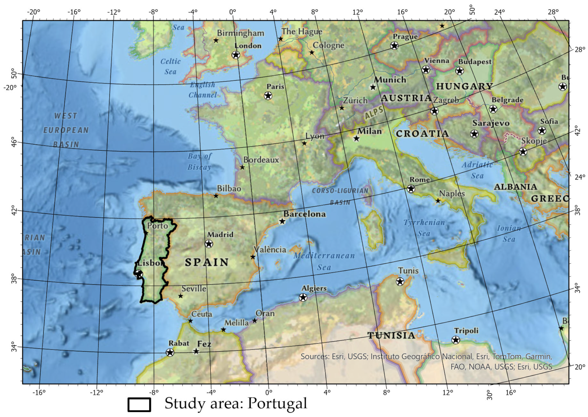
In this paper, we report the results of the thematic accuracy of six 10 m spatial resolution LULC products (global, continental and national) for the same study area: continental Portugal. The thematic accuracy assessment evaluates the following: (1) the original products and all their original classes, hence enabling a comparison between the quality of original products; (2) the accuracy of the harmonized maps obtained from the original products considering a harmonized nomenclature; (3) a direct comparison of the characteristics of the harmonized products.

The reference database used to validate the products was generated considering the good practices’ recommendations for accuracy assessment. To assure that reference database could be used to assess the thematic accuracy of all original products, a stratified random sample, e.g., [29], was generated with strata extracted from existing ancillary data that provided enough detail to be mapped into the original classes of all products. This enabled the generation of a reference database independently of the products to validate, while overcoming the limitations of a simple random sample that would not provide enough sample units in the rare classes. In the response design phase, classes had to be used that could be mapped onto the original classes of all products. Therefore, nineteen classes were used in the reference database. Moreover, the considered methodology enables the quantification of the effect of the uncertainty in the selection of the “true class” for each sample unit, by selecting a primary and secondary class whenever necessary [20,21,22,23]. The accuracy indices were then computed using the accuracy estimators applicable to the validation of maps when a sampling design uses strata different from the map classes [30].

The work presented in this paper is structured as follows: The characteristics of the study area and the products under analysis are presented in Section 2. The methodology used to assess the thematic accuracy of the original maps, the methodology to obtain the harmonized maps, their accuracy and their comparison is described in Section 3. The results are presented in Section 4, discussed in Section 5 and conclusions are drawn in Section 6.

2. Study Area and Datasets

2.1. Study Area Characterization

The study area is continental Portugal in the Iberian Peninsula, located in the south-west of the European continent (Figure 1), covering an area of approximately 90,000 km². Continental Portugal has a temperate climate with Atlantic and Mediterranean influences, respectively in the North and South regions, with cold and traditionally wet winters and hot dry summers. It can be divided into three distinct regions [31]: (a) the north-western region, which is also the Portuguese region with the higher population density and a fine-grained mosaic of land use; (b) the north-eastern region, drier than the previously described region, composed of mountains, with a lower population density, large farmland and forest patches, divided into small ownership familiar agriculture and forested fields; (c) the southern region, with a Mediterranean influence, large plains and farms. In these regions, large extents are covered by an open oak woodland with agro-silvo-pastoral use, which contributes to a more homogeneous landscape.

2.2. Datasets

This study analyses six raster LULC maps available for continental Portugal with 10m spatial resolution and similar time stamps. However, they have some differences regarding the reference date (the maximum time difference between the analyzed products is 3 years), the used nomenclatures, validation procedure and geographical extent of the validation. Figure 2 shows the maps with their original nomenclatures and the classes available for continental Portugal. An additional LULC map, described at the end of this section, was used to define strata to generate the reference database generated to assess the product’s thematic accuracy.

2.2.1. Land Cover Map of Europe 2017 (S2GLC)

S2GLC [32] was generated through the automatic classification of Sentinel-2 images for the reference date of 2017, considering imagery from January to December 2017 [13]. It maps 13 land cover classes at 10 m spatial resolution for a major portion of the European continent. The S2GLC is the output of a project funded by the European Space Agency (ESA) through the Scientific Exploitation of Operational Missions. Details regarding the validation are presented in Malinowski et al. [13]. Overall, a total of 51,926 validation samples were collected over the extent of the dataset, having in mind that each of the countries would have a minimum set of points. The thematic accuracy achieved an overall accuracy of 86% for the whole extent of the map. The authors further indicated that the best accuracy was achieved for the “Evergreen coniferous tree cover” class, while “Permanent snow and glaciers” and “Sclerophyllous vegetation” were the ones presenting the worst metrics. For Portugal, the authors report an overall accuracy of 67%, which is derived from 890 sampling points, extracted from a single Sentinel-2 tile (tile 29TNE) within continental Portugal. The whole product can be downloaded in the European Terrestrial Reference System 1989 (ETRS 89).

2.2.2. ESRI 2020 Land Cover (ESRI LC)

ESRI LC [33] is a global product, mapping 10 classes for the reference year 2020 (considered data comprising the whole year) at a 10 m spatial resolution using Sentinel-2 images (see Figure 2). The validation was performed building a confusion matrix by comparing the resulting map with 409 validation tiles covering 5 km × 5 km sample areas over the globe, which were built using three annotators. An overall accuracy of 86% for the global map was reported. Accuracy metrics for several countries are also available [14]. According to these metrics the best performing class was “Trees” while the worst was “Grass”. The map is available for free download and is delivered using the Universal Transverse Mercator (UTM) coordinate system. There are also updated versions of the ESRI LC for the reference years 2021 and 2022.

2.2.3. Carta de Ocupação do Solo Conjuntural 2018 (COSc)

COSc (formerly called COSsim) is a product produced by the Portuguese National Mapping Agency (Direção-Geral do Território—DGT) [34]. The objective of this product is to map 13 classes annually using semi-automated methods, combining expert rules with the image classification of Sentinel-2 satellite imagery. The accuracy of this product is only available for the 2018 version [35]. To accommodate the 2018 agricultural year, the data considered for the 2018 map was collected from October 2017 to September 2018. The authors indicate an overall accuracy of 81.3% with a confidence interval of 2.1%. The classes showing the best accuracy were “Water”, “Evergreen oaks”, “Agriculture” and “Eucalyptus”, while the ones showing the worst accuracy metrics were “Bare soil” and “Conifers”. COSc can be downloaded from the SNIG (Sistema Nacional de Informação Geográfica—National System of Geographic Information) web page in the official Portuguese reference system: PT-TM06 ETRS89 (EPSG: 3763).

2.2.4. CLC+ Backbone (CLC+ BB)

The CLC+ BB [36] is the first version of the first stage product of the CLC+ new approach to produce LULC information [37]. The first version for the whole of Europe was made available in 2023 for the reference year of 2018 (considered data from July 2017 to June 2019). The thematic accuracy of the product is not yet available. It is a raster product with a 10 m spatial resolution and 11 land cover classes (from which only nine exist in Portugal) (see Figure 2) following the EAGLE classification concept [38]. The product is available in the ETRS 1989, Lambert Azimuthal Equal Area projection (ETRS 89—LAEA) (EPSG code: 3035).

2.2.5. ESA WorldCover 2020 (ESA WC)

ESA WC 2020 [39] is a global land cover product for the reference year 2020 (considered data from January to December 2020), mapping 11 land cover classes (from which only eight exist in Portugal) with a spatial resolution of 10 m. Like the other products, it was produced using image recognition methods having as its input Sentinel-1 and Sentinel-2 data. The statistical accuracy assessment used the Copernicus Global Land Service Validation data [40] which is based on probability sampling. The validation data contain more than 20,000 primary sampling units (PSU) corresponding to 100 m × 100 m square spatial units. Each of these PSU were divided in 10 × 10 m blocks denominated secondary sampling units (SSU). The overall accuracy obtained for Europe (EU) was 76.8 ± 0.2%, computed with a total of 3118 PSU and the corresponding SSU. The product is available for free, downloaded in geographical coordinates in the World Geodetic System 1984 (WGS 84) (EPSG code: 4326) where a 2021 version already exists.

2.2.6. ELC10 2018

The ELC10 2018 (ELC10) is a European land cover product mapping eight classes with a 10 m spatial resolution [15]. It was produced by the Norwegian Institute for Nature Research and generated from image classification methods using Sentinel-2 images. The validation was made using 25,000 reference points within Europe [15] and an overall accuracy of 90% was obtained. The class showing the worst accuracy results was “Shrubland” while the highest was “Artificial land”. The map is available for download in ETRS89/LAEA Europe reference system (EPSG:3035) for the reference year of 2018 (considered data from the whole year).

2.2.7. COS 2018

Carta de Uso e Ocupação do Solo (COS) is the main LULC product generated by the Portuguese National Mapping Agency—DGT [41]. It is a vector product with 83 classes (divided in four levels of detail) focused on land use, with a minimum mapping unit of 1 ha, generated using the photo interpretation of aerial orthophotos with a 0.25 m spatial resolution. Given the slow and costly campaign necessary to produce such product, it is only produced every 3 to 5 years. Technical specifications indicate that the thematic accuracy should be equal to or better than 85% [42]. Due to the very different characteristics of this product in relation to the other products under analysis, COS 2018 was only used in this analysis to identify strata for the sampling strategy used to generate the reference database necessary for the accuracy assessment of the products under analysis. The product is available for download in PT-TM06/ETRS89 reference system (EPSG: 3763) at the site of DGT [41].

3. Methodology

The methodology used to validate and compare the LULC maps described in the previous section includes three phases, illustrated in Figure 3.

The first phase corresponds to the accuracy assessment of the original products with a reference database. The methodology used to generate the reference database and compute the accuracy indices is fully described in Section 3.1, along with the used accuracy indices.

The second phase aims to assess the accuracy of the harmonized maps with the reference database generated in Phase 1. To this aim, after the class definitions were analyzed, the nomenclatures of the six LULC maps were converted into a common and comparable nomenclature, henceforth referred to as harmonized nomenclature (HN). All maps were then converted into this HN generating harmonized and comparable maps. Then, accuracy indices were computed for the harmonized maps derived from each of the original maps, using the reference database generated in Phase 1. The details of the methodology used in this phase are further explained in Section 3.2.

The third phase corresponds to the direct comparison of the harmonized maps, with the identification of similarities and differences between the products, in particular the area occupied by each corresponding class in each map and the regions equally mapped in all harmonized maps. Further explanations of this process are made in Section 3.3.

3.1. Thematic Accuracy Assessment of the Original LULC Maps

Given the number of products to validate and the aim to compare the obtained accuracy results, the same reference database was used to validate all products, so that accuracy differences would not be due to the use of different reference databases. To consider a different reference database for each map would, on one hand, introduce variability in the accuracy results and, on the other hand, would significantly increase the effort and costs necessary to generate six reference databases. Therefore, the reference dataset was designed in such a way that it enables the assessment of the accuracy of each original LULC map, with its own nomenclature. The methodology used to generate this reference database and validate the products is described in this section and includes the three main steps of accuracy assessment, namely: (1) sampling design; (2) response design; (3) computation of accuracy indicators.

3.1.1. Sampling Design

The sampling design defines the protocol to select the reference spatial units where the “true class” will be identified and then compared with the map classes. Several sampling approaches may be used for this aim, such as simple random, systematic or stratified sampling, but all have advantages and disadvantages, e.g., [29,43]. In this analysis, a stratified random sample of points was used. The stratified sampling approach satisfies several major design criteria regarding the sampling design: (1) it follows a probability sampling design, (2) it is cost-effective and practical by reducing the number of sampling points, (3) it enables the distribution of the sampling points in strata that represent the diversity of the landscape under analysis, (4) it enables the collection of sample data at rare classes. The strata most commonly used when validating a LULC map are the map classes. However, due to the different classes used in the products under analysis, such an approach would result in the identification of a different set of sampling points for each map. These could then be merged into only one reference database but the points selected in each one would have different selection probabilities, which would make the accuracy assessment more complex, and would also increase the sample size and therefore the effort and cost of the response design phase. Hence, it would neither be practical nor cost-effective, which are two major criteria when selecting the sampling design [29]. Therefore, the strata were defined by using 19 classes, listed in

Table 1. The 19 classes extracted from COS 2018 used to define the strata considered in the stratified random sampling approach to create a reference database, their level of detail in the COS 2018 hierarchic nomenclature (with 4 levels) and the area they occupy in the study area (in km²).

COS 2018 Nomenclature Level	Class Name	Area (km2)
1	Artificial surfaces	4324
2	Annual croplands	14,558
3	Vineyards	1944
3	Orchards	1843
3	Olive groves	4506
3	Managed grasslands	5442
3	Spontaneous herbaceous vegetation	767
1	Agroforestry surfaces	7469
4	Holm and cork oak	7924
4	Eucalyptus	9286
4	Other oak trees	2240
4	Other broad-leaved trees	2480
4	Maritime pine	10,194
4	Stone pine	2009
4	Other pine trees	370
1	Shrublands	11,086
1	Surface without vegetation or with sparse vegetation	869
1	Wetlands	264
1	Water	1385

, extracted from the 83 classes of COS 2018, described in Section 2.2.7, and considered in this study as reflecting the diversity of the landscape in Portugal.

These strata were selected so that all classes of the original LULC maps would be represented in the selected sample.

For each of the selected strata, 60 sampling units were randomly selected. Therefore, the reference database includes a total of 1140 points. In spite of the use of the main landscape components of continental Portugal as strata, with such a sampling approach, there may be land cover classes in some products that have less samples, which is not desirable as it will increase the amplitude of the confidence intervals associated with the accuracy indices, e.g., [44,45]. However, as the alternative would require a very large reference database, this was the chosen option. The reference system used in the reference database was the PT-TM06/ETRS89 (EPSG code: 3763). Figure 4 shows the obtained reference points and the considered strata.

3.1.2. Response Design

The response design defines the protocol used to select the reference class at each sample location, frequently called “ground truth” class. It involves several aspects, including the selection of the reference classes that may be used and the method and rules used to select the “true class” or the possible “true classes” at each reference location [46].

The reference database used in this study was generated by selecting the reference class for each LULC product (considering their original classes) through the photo interpretation of the 2018 orthorectified aerial images with 0.25 m spatial resolution, along with the ones available for the years 1995, 2004–2006, 2007, 2010, 2012 and 2015, and a time series of Sentinel-2 satellite imagery between 2017 and 2019. Additional data were also used, such as the burned areas between 2017 and 2019 provided by the Portuguese National Institute for Nature and Forest Conservation (Instituto da Conservação da Natureza e das Florestas—ICNF) and the Portuguese Land Parcel Identification System (Sistema de Identificação Parcelar) of the Institute for Funding Agriculture and Fishery (Instituto de Financiamento da Agricultura e Pescas—IFAP). The use of all these data sources enabled the photointerpreters to consider variability when selecting the reference class, as the identification of some classes, such as “Agriculture”, “Permanent herbaceous” or “Periodically herbaceous” require an analysis of variability over time.

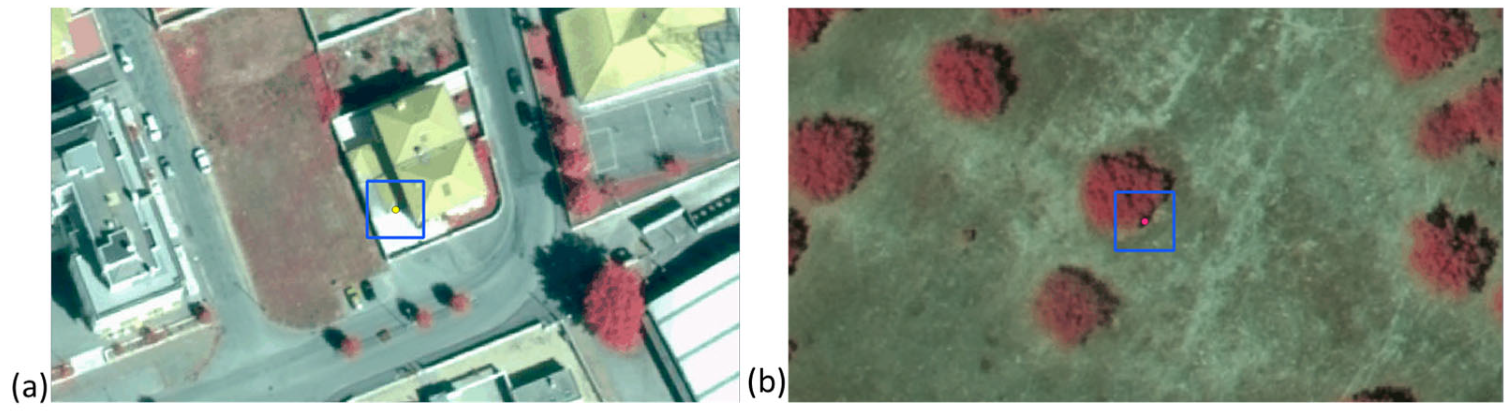
Given that the maps to be validated have a 10 m spatial resolution, a 100 m² square cell centered around the sample point was considered to identify the reference class. The four interpreters performing this work were instructed to choose the reference class that was dominant in the considered 100 m² cell. When more than one class was present in the cell, the one with larger percentage (equal or larger than 60%) was considered as the primary class and a secondary class could be chosen (corresponding to the remaining 40%). In rare cases where it was very difficult to identify the dominant class in the cell, the interpreter labeled the sample point considering the area surrounding the square cell. Figure 5 illustrates this procedure with two examples. In (a) there is no doubt that the class to be selected should be “Artificial Land”, while in (b) it was not possible to choose which of the classes “Permanent herbaceous” and “Woody Broadleaved evergreen trees” was dominant in the cell. In this case, the region surrounding the cell was considered to choose the class “Permanent herbaceous” as primary and the class “Woody broadleaved evergreen trees” as the secondary class.

A secondary class was selected for 48% of the 1140 considered sample units.

Table 2. Percentage of sample units per strata for which a secondary class was considered.

Class Name (Strata)	Sample Units with Secondary Class (%)
Artificial surfaces	65
Annual croplands	40
Vineyards	80
Orchards	73
Olive groves	80
Managed grasslands	18
Spontaneous herbaceous vegetation	38
Agroforestry surfaces	50
Holm and cork oak	57
Eucalyptus	50
Other oak trees	58
Other broad-leaved trees	42
Maritime pine	62
Stone pine	37
Other pine trees	42
Shrublands	28
Surface without vegetation or with sparse vegetation	47
Wetlands	43
Water	5

shows the percentage of the 60 sample units per strata for which a secondary class was identified. These values show the difficulty to select one class for pixels with 100 m², as, due to the landscape characteristics, many pixels are in fact mixed pixels. It is also clear that some strata are less sensitive to this difficulty, such as Water and Managed grasslands, due to their homogeneity.

To solve any doubts that might occur in the photo-interpretation phase, in the first step, three photo interpreters classified the same 10 sampling points from each of the strata, adding up to 190 points. The results allowed us to identify divergencies between photo interpreters, and additional rules were defined to assess these situations. Afterward, the remaining points were split using the same three interpreters for labeling, assuring that all photo interpreters had points from all strata. In the end, all the points were revisited by a fourth photo interpreter and a meeting was held between the four interpreters to solve any remaining inconsistencies between them.

3.1.3. Accuracy Indicators

The computation of accuracy indices requires the comparison, at each sample location, between the reference class and the map class. As the different maps were originally available in different reference systems, to minimize the impact of possible displacements, distortions and the need to resample pixels when applying transformations between reference systems, the reference database reference system was converted into the reference system of the original LULC maps to be validated.

The comparison between the LULC maps and the reference data is made building confusion matrices. However, as the strata used to select the sample points are not the classes of the maps to be validated, the confusion matrices need to keep the information about the class in the map and the reference data, but also about the original strata that contained each reference point. Therefore, the overall accuracy is estimated using Equation (1), its standard deviation is estimated with Equation (2), the user’s and producer’s accuracy are estimated using Equation (3) and their standard deviations are estimated using Equation (4), and the estimation of the area of class j e is given by Equation (5) [30],

$$\widehat{\overline{Y}}={\sum }_{h=1}^H\frac{N_h^{*}\overline{y_h}}{N}$$

(1)

$$\widehat{SD}\left(\widehat{\overline{Y}}\right)=\sqrt{\frac{1}{N^2}{\sum }_{h=1}^H\frac{N_h^{*2}\left(1-\frac{n_h^{*}}{N_h^{*}}\right)s_{yh}^2}{n_h^{*}}}$$

(2)

$$\widehat{R}=\frac{{\sum }_{h=1}^H{N}_h^{*}\overline{y_h}}{{\sum }_{h=1}^H{N}_h^{*}\overline{x_h}}$$

(3)

$$\widehat{SD}\left(\widehat{R}\right)=\sqrt{\frac{1}{{\widehat{X}}^2}{\sum }_{h=1}^H\frac{N_h^{*2}\left(1-\frac{n_h^{*}}{N_h^{*}}\right)\left(s_{yh}^2+{\widehat{R}}^2{s}_{xh}^2-2\widehat{R}{s}_{xyh}\right)}{n_h^{*}}}$$

(4)

$$\widehat{A_j}=\frac{A}{N}{\sum }_{h=1}^H{N}_h^{*}\overline{z_h}$$

(5)

where:

• N is the total number of sample units;
• H is the number of strata;
• h is one of the H strata;
• $N_h^{*}$ is the amount of sample units within stratum h;
• u represents a sample unit;
• A is the total area of the map;
• $y_u$, $x_u$ and $z_u$ are variables that take values either 1 or 0, such that:

To compute the overall accuracy:

$$y_u=\left\{\begin{array}{l}1 \Leftarrow pixel u is correctelly classified \\ 0 ⟸otherwise\end{array}\right.$$

To compute the user’s accuracy of class k:

$$y_u=\left\{\begin{array}{l}1 \Leftarrow pixel u is correctelly classified in the map as class k\\ 0 ⟸otherwise\end{array}\right.$$

$$x_u=\left\{\begin{array}{l}1 \Leftarrow pixel u belongs to class k in the map\\ 0 ⟸otherwise\end{array}\right.$$

To compute the producer’s accuracy of class k:

$$y_u=\left\{\begin{array}{l}1 \Leftarrow pixel u is correctelly classified and has reference class k\\ 0 ⟸otherwise\end{array}\right.$$

$$x_u=\left\{\begin{array}{l}1 \Leftarrow pixel u belong to reference class k \\ 0 ⟸otherwise\end{array}\right.$$

To compute the estimation of the area of class j:

$$z_u=\left\{\begin{array}{l}1 \Leftarrow pixel u belong to reference class j \\ 0 ⟸otherwise\end{array}\right.$$

• $\overline{Y}=\frac{{\sum }_{u=1}^H{y}_u}{N}$ is the population mean based on a census of $N$ pixels;
• $\widehat{\overline{Y}}$ estimator of $\overline{Y}$;
• $\widehat{R}$ estimator of the ratio $R=\frac{{\sum }_{u=1}^H{y}_u}{{\sum }_{u=1}^H{x}_u}$;
• ${\overline{y}}_h={\sum }_{u\in h}\frac{y_u}{n_h^{*}}$ is the average of $y_u$ for the sample units in stratum $h$;
• $n_h^{*}$ is the amount of sample units which were selected from stratum $h$;
• ${\overline{x}}_h={\sum }_{u\in h}\frac{x_u}{n_h^{*}}$ is the average of $x_u$ for the sample units in stratum $h$;
• ${\overline{z}}_h={\sum }_{u\in h}\frac{z_u}{n_h^{*}}$ is the average of $z_u$ for the sample units in stratum $h$;
• $s_{yh}^2={\sum }_{u\in h}\frac{{\left(y_u-\overline{y_h}\right)}^2}{n_h^{*}-1}$ is the sample variance of $y_u$ from stratum h;
• $s_{xh}^2={\sum }_{u\in h}\frac{{\left(x_u-\overline{x_h}\right)}^2}{n_h^{*}-1}$ is the sample variance of $x_u$ within stratum h;
• $s_{xyh}={\sum }_{u\in h}\frac{\left(y_u-\overline{y_h}\right)\left(x_u-\overline{x_h}\right)}{n_h^{*}-1}$ is the sample covariance between $x_u$ and $y_u$ for stratum h;
• $\widehat{X}={\sum }_{h=1}^H{N}_h^{*}{\overline{x}}_h$.

The 90% confidence intervals (CI₉₀) were computed using Equation (6), where SD stands for standard deviation and EA for the estimated accuracy.

$${CI}_{90}=\left[EA-1.645\ast SD,EA+1.645\ast SD \right]$$

(6)

The accuracy indices were computed following the two approaches below, given that the reference database considers not only a primary class but, in some cases, also a secondary class.

• There is an agreement between the map and the reference data only when the map pixel that contains the reference point is coincident with the primary class of the reference database;
• There is an agreement between the map and the reference data when the map pixel that contains the reference point is coincident with the primary or the secondary class of the reference database.

As the second approach considers that there is agreement in more cases than the first one, the accuracy results are always equal or higher than the ones obtained with the first approach. This second approach also aims at decreasing the effect of small co-registration problems between the products and the reference database.

As the products under comparison have different classes, and also a different number of classes (three products have only eight classes, and there is one with nine classes, another with eleven and another with thirteen classes), the simple comparison of the overall accuracy does not provide enough information for a user to assess which product is more likely to provide accurate information for a particular application. Moreover, when the analysis is made per class, very different accuracy values may be obtained for the user’s and producer’s accuracy indices, which means that there may be very different levels of omission and commission errors in each map for each class. To help to assess which product has more classes that show a high level of reliability regarding both omission and commission errors, the F1-score per class was computed, e.g., [47]. This measure is computed for each class with Equation (7), where $c$ represents the class under assessment, and $UA\left(c\right)$ and $PA\left(c\right)$ represent, respectively, the user’s and producer’s accuracy of class $c$.

$${F1}_c=\frac{2\ast UA\left(c\right)\ast PA\left(c\right)}{UA \left(c\right)+PA\left(c\right)}$$

(7)

This measure enables to assess the quality of each class in each map separately. This is useful to assess if a certain map may be a good data source for a particular class or not independently of its performance in other classes, which may not be of interest for a particular application.

3.2. Nomenclature Comparison and Harmonization

All maps under analysis have different nomenclatures, with classes that may be land-cover oriented, land-use oriented, or a mixture of both. Therefore, to perform the nomenclature harmonization it is necessary to analyze the definitions of LULC classes of each product. Then, to generate maps that can be compared, a set of classes into which the original classes of the products may be mapped needs to be identified.

Table 3. Mapping between the harmonized nomenclature (HN) and the original classes of each product, existing in continental Portugal.

HN	ESRI LC	ESA WC	ELC10	CLC+ BB	S2GLC	COSc
Built area	− Built area	− Built-up	− Artificial Land	− Sealed	− Artificial surfaces	− Artificial Land
Vegeteted area	− Crops	− Cropland	− Cropland	− Periodically herbaceous	− Cultivated areas − Vineyards − Artificial surfaces	− Agriculture
	− Trees	− Tree Cover	− Woodland	− Woody Broadleaved deciduous trees − Woody Broadleaved evergreen trees − Woody needle leaved trees	− Broadleaf tree − Coniferous tree	− Evergreen oaks − Eucalyptus − Other broadleaves − Stone pine − Maritime pine − Other conifers
	− Scrub/shrub	− Shrubland	− Shrubland	− Low-growing woody plants	− Moors and Heathland	− Shrubland
					− Sclerophyllous vegetation
	− Grass − Flooded vegetation	− Grassland − Herbaceous wetland	− Grassland − Wetland	− Permanent herbaceous	− Herbaceous vegetation − Marshes	− Natural grassland − Wetland
Bare land	− Bare ground	− Bare/sparse vegetation	− Bare Land	− Non and sparsely vegetated	− Natural material surfaces	− Bare soil
Water	− Water	− Permanent water bodies	− Water	− Water	− Water bodies	− Water

shows the mapping of all classes of the six products under analysis into the classes considered in the HN. This mapping enables a direct comparison of the maps obtained once the original products are reclassified into this common nomenclature. However, due to the difficulties associated with the class’s definitions in the several products, which make correspondences difficult in several cases as the same land cover may be included in different classes due, for example, to different land uses, only four classes were considered in the HN, which are “Built area”, “Vegetated areas”, “Bare ground” and “Water”. Most of the difficulties that implicated the choice of only four classes are in the vegetated classes, which may include, for example, vineyards in different classes (in some cases they correspond to a separate class, in others they are included in agriculture and in other in shrubs). Similar difficulties are found for LULC classes, such as orchards (which in some cases are included in the trees class and in other cases in agriculture) and other types of vegetation, so only one class was considered for all vegetated areas. All products were then converted into the classes of the HN.

To assess the accuracy of the harmonized products, the reference database generated in Section 3.1 was used. As each sample point was already associated with the classes of each original product, additional attributes were added to the reference database with the corresponding classes of the HN, according to the mapping listed in Table 3. As the classes of the harmonized maps to be validated also do not correspond to the strata used to select the sample points, Formulas (1)–(4) were used to compute the accuracy indices, as explained in Section 3.1.3.

3.3. Comparison of the Harmonized Maps

To enable a direct comparison of all harmonized maps, they were converted into the same reference system (PT-TM06/ETRS89—EPSG code: 3763). Three types of analysis were then performed: (1) a comparison using visual analysis, (2) the area occupied by each class in each harmonized map was computed and the results obtained for all maps compared, (3) the regions classified with the same harmonized class in all maps was identified, the area per class was computed, as well as the percentage of regions equally classified in relation to the minimum and maximum class area in all maps.

4. Results

4.1. Accuracy of the Original Products

4.1.1. Accuracy Values Obtained with the Created Reference Data

The overall accuracy of the original LULC maps, computed as explained in Section 3.1, are shown in Figure 6. The 90% confidence intervals of the accuracy values are also shown.

The results show that the original maps with larger overall accuracy are CLC+ BB and COSc, with the first one only 1% larger than the second when the primary and secondary classes are considered to identify agreement between the map and the reference dataset (72% versus 71%), even though COSc has thirteen classes and CLC+ BB has only nine classes for the study area. This difference has a small significance, as the 90% confidence intervals are almost completely overlapping, both with an amplitude of 6%. When only the primary class is considered, the overall accuracy decreases to 62% and 58%, respectively, for CLC+ BB and COSc, corresponding to a difference of 4%. The product with the lowest overall accuracy is ESRI LC.

The user’s and producer’s accuracy per class of all original LULC maps, as well as the 90% confidence intervals associated with each obtained value, are shown in Figure 7. The main aspects that stand out are:

• In most maps and classes, the difference obtained when using only the primary class of the reference database or the primary and secondary class are relatively small (lower than 10%). However, some exceptions to this are observed. The most relevant cases correspond to the user’s accuracy of the classes “Cork-oak and Evergreen-oak” and “Maritime pine” in COSc. These differences are due to the characteristic of landscape where these types of trees exist, illustrated in Figure 5b, where the trees are distant from each other with low vegetation in between. Therefore, most pixels in these areas will be mixed, and the secondary class may in fact raise the chance of agreement between the reference data and the map.
• The map with more inaccurate classes is ESRI LC. The accuracy results per class enable to understand what was observed for the overall accuracy, as there are large commission errors in the class “Built area” and large omission errors in the classes “Bare ground” and “Grass”.
• In all products, the classes with better user’s and producer’s accuracy are the water classes.
• The classes associated with agriculture are better mapped in COSc. The second-best results for this land cover are obtained for CLC+ BB, as the class that includes the agriculture areas, which change between vegetated areas and bare land, in CLC+ BB is the class “Periodically herbaceous”. This class has the user’s accuracy higher than 80%, but the producer’s accuracy lower than 60%, which indicates omission errors. However, due to the land cover characteristics of this product, other classes may also include agriculture areas, which may be mapped to shrublands (e.g., vineyards) or trees (e.g., orchards or olive trees).
• The most problematic classes in S2GLC is the class “Vineyards”, with very large commission errors.
• In some maps there are classes with wider confidence intervals. For example, the class “Wetlands” at ELC10, or the class “Grass” in ESRI LC. These problems may originate from the limitations associated with the sampling design, which resulted in less sample points in these classes.

To assess the capacity of each product to provide a good source of data for some classes, the F1-score was computed, using Equation (7), for each class and each product (see Figure 8).

The number of classes per product with the F1-score belonging to the five 20% equal range intervals defined between 0% and 100% are shown in Figure 9. It stands out that the product with more classes in the [80%, 100%] interval (which means that both the UA and the PA of the class are very high) is COSc (with five classes in this interval), followed by ESA WC (with three classes), CLC+ BB (with two classes) and S2GLC (with only one class). Regarding the interval [60%, 80%], both COSc and CLC+ BB have six classes with an F1-score in this range, followed by S2GLC, with five classes. All products have classes with an F1-score lower than 40%, which in all products correspond to classes of bare ground or areas with grass or sparsely vegetated areas, with two exceptions, which are “Shrubland” in ESA WC (F1 = 37%) and “Vineyards” in S2GLC (F1 = 25%) (see Figure 8).

4.1.2. Comparison with Accuracy Values Reported by Map Producers

The accuracy metrics presented in the previous section are compared with the accuracy values reported by each of the map producers. However, given the number of different maps considered in this study and the different map producers, such accuracy metrics are performed differently and assessed considering different geographical extents as explained in Section 2.2.

Figure 10 enables the comparison of the overall accuracy of the several products obtained in this study and the results reported, for Portugal, Europe or globally, depending on what is available. Regarding S2GLC, the results are available in Venter and Sydenham [15] for Europe and Portugal (Figure 10a). The results obtained for Portugal are almost 20% lower than the ones obtained for Europe, and they are even lower with the methodology used in this paper. Given that the 90% confidence interval obtained in this study for the overall accuracy has an amplitude of ±3%, the accuracy results reported for Portugal with the stratification by country described in Venter and Sydenham [15] probably does not capture the classification errors in the more problematic classes. The overall accuracy obtained for Portugal with the methodologies used in this paper for ESRI LC (Figure 10b) is much lower than the ones reported globally. The same happens for ESA WC (Figure 10c) and to ELC10 (Figure 10d) when comparing with the results available for Europe, with differences even larger for this last product.

Regarding the user’s and producer’s accuracy per class, for the S2GLC they are only published for the whole extent of the map (not per country) and are plotted in Figure 11, along with the results obtained in this paper.

When comparing the European wide values with the ones reported here some differences stand out. On one hand, the classes “Cultivated areas”, “Broadleaf tree”, “Coniferous tree” and “Natural material surfaces” have much higher user’s and producer’s accuracies in the European assessment than the results obtained for Portugal. The opposite occurs with the class “Marshes” and the producer’s accuracy of the class “Sclerophyllous vegetation”. Even though the class “Vineyards” has low user’s accuracy for all Europe, the values obtained in this study are even lower, which indicates very large commission errors in Portugal.

The user’s and producer’s accuracy per class obtained in this study and reported for Europe for ESA WC [17] are shown in Figure 12. The most significant differences observed are a lower PA for the class “Cropland” than the one reported for Europe, higher PA regarding “Grassland” and a much higher PA and UA for the “Herbaceous wetland” class.

The user’s and producer’s accuracy per class obtained in this study and for Europe for ELC10 [15] are shown in Figure 13. The results reported in this document are always much lower than the ones obtained for Europe, where classes “Bare land” and “Wetland” are the ones with larger differences and the classes “Water”, “Artificial land” and “Woodland” are the ones with lower differences.

The user’s and producer’s accuracy obtained per class in this study and the global values reported for ESRI LC [14] are shown in Figure 14. Very large values of the user’s accuracy are observed globally for the classes “Built area”, “Crops” and “Scrub/shrub” when compared with the ones obtained in this study, independently of the methodology considered. The same is observed for the producer’s accuracy of the classes “Bare ground” and “Grass”. On the other hand, the user’s accuracy of these classes obtained in this study are much higher than the values reported globally. This shows that there are very large omission errors in these classes in ESRI LC for Portugal.

CLC+ BB still does not have a validation report available that enables a comparison with the results reported here. Regarding COSc, it is a national product, so there are no results for other regions outside Portugal.

Overall, the accuracy values reported by the map producers are in general higher than the ones obtained in this study for the area under analysis. To this regard, the literature indicates that southern-European landscapes are often mapped with lower accuracy scores [15,48]. Moreover, in the recent literature, which compared some of the used maps such as ESRI LC and ESA WC within country wide assessments, also showed the overestimation by ESRI LC of the “Built area” class and the underestimation of the “Shrubland” class in ESA WC [18,19].

4.2. Accuracy of the Harmonized Products

The overall accuracy of the maps with the HN obtained from each product, along with the 90% confidence intervals, are shown in Figure 15.

Due to the classes’ aggregation, the overall accuracy of all maps increases to more than 83%, reaching 95% for the ELC10 when the primary or secondary class are considered. It stands out that the overall accuracy of the harmonized product generated from the ELC10 is very high. This was not the case with the original product, which had an overall accuracy of only 48% when only the primary class was considered and 61% when the primary or secondary class were considered. This occurs because the major source of errors in this product is the confusion between types of vegetation, as shown by the low values of user’s and/or producer’s accuracy of the vegetated classes when compared with the accuracy of the class “Artificial land” and “Water” (see Figure 7 and Figure 8).

The user’s and producer’s accuracy per class of the harmonized maps are shown in Figure 16. It can be seen that all products have a high accuracy for the “Vegetated areas”, which corresponds to most of the study area. The class “Bare land” is mapped with lower accuracy in all products. The user’s accuracy of the class “Water” is similar in most products, with slightly worse values in ESRI LC and ELC10 and wider confidence intervals than for the other products. The class “Built area”, has similar accuracy in S2GLC, COSc, ESA WC and ELC10, and better producer’s accuracy (less omissions) in the CLC+ BB, and large commission errors at ESRI LC. However, due to the large difference between the user’s and producer’s accuracy for ESRI LC, it appears to overestimate the built areas.

The F1-score, computed for all classes in all products, is shown in Figure 17. The very similar F1-scores for the vegetated areas confirm that this class is well mapped in all products, and the low F1-score confirms the low quality of the class bare land in all maps, with particular emphasis in the ESRI LC product. No big differences are observed regarding the class water, but more differences are observed for the class build-area, especially for ESRI LC.

These results show that small accuracy differences are obtained for the harmonized products. However, the accuracy indices are not able to express some relevant differences that may be important when deciding which product to use for a particular application. Therefore, a further comparison of the obtained harmonized products in made in the next section.

4.3. Comparison of the Harmonized Maps

4.3.1. Visual Comparison

The LC maps obtained with the mapping of the original LULC maps into the four classes of the HN described in Section 3.2 can be seen in Figure 18. Figure 19 shows the region highlighted with a rectangle in Figure 18, where the differences can be seen in more detail.

The main information that may be obtained from the country wide maps shown in Figure 18, is that (1) most of the country is mapped as vegetated area in all maps, (2) the class “Bare land” occupies small areas in all maps, (3) the major water areas appear to be represented in all maps, and (4) there is a very large difference between the built area mapped, mainly in the ESRI LC map and all other products, confirming that this class must be overestimated in this product.

The analysis of the more detailed areas shown in Figure 19 enables the identification of additional differences between the obtained maps. There are differences related to the area, level of detail and continuity of the classes and features they represent in the several maps.

The main feature that stands out is the difference between the ESRI LC derived map when compared with the other maps, which has much larger built areas showing lower detail. The level of detail observed in all other maps regarding the built areas is more similar, even though a closer look starts to show differences, such as, for example, the lack of continuity in the representation of roads.

The map that shows roads with higher detail is the one derived from CLC+ BB. The second map showing a higher level of road continuity is the one derived from COSc. ESA WC also shows some clearly identified roads, while ELC10 and S2GLC derived products show much less continuity in this type of infrastructure.

Large differences between the maps can also be seen in the classification of “Bare land”. The region identified with the back ellipse in Figure 19 has been classified in some maps as “Built area” and in others as “Bare land”. Figure 20 shows the 2018 orthorectified aerial images of the region represented in Figure 19, where the area inside the ellipse stands out. In fact, this region corresponds to a quarry associated with a cement factory, and therefore, according to the class’s definition, it should be classified as “Bare land” in S2GLC and ESA WC instead of “Built area”. Therefore, this difference is not due to a mistake but to different classes’ definitions.

The region near the water body on the right lower part of Figure 19 is shown in more detail in Figure 21. Another difference that can be easily noticed in the maps of these figures (Figure 19 and Figure 21) is the difference in the classification of “Bare land” in all maps. CLC+ BB contains more regions classified as bare land spread along the area, while, for example, S2GLC shows very few bare areas.

The class that shows more similarity in all maps is the “Water” class, which is not surprising due to the less likely confusion with the other classes. However, some smaller water areas, such as narrower water lines are in some maps omitted (e.g., S2GLC and ESA WC) and in others only some pixels of these water bodies are classified as “Water”, but with no continuity (ELC10 and ESRI LC).

4.3.2. Comparison of the Regions Equally Classified and Class’s Areas

The regions that were equally classified when converting the original LULC maps into the four classes of the HN are represented in Figure 22. These regions correspond to 83% of the study area.

The areas of the classes considered in the HN for the maps obtained from the six original LULC products for continental Portugal, along with the estimated area of each class computed with the area estimator given by Equation (5), are shown in Figure 23. Even when only the four harmonized classes are considered, the results obtained from the different maps show area differences that, in some classes, are very large. In agreement with the visual analysis, the map with the largest differences in relation to all others is the one derived from the ESRI LC product, which has a much larger area classified as “Built area” and much smaller areas classified as “Vegetated areas” and “Bare land” than all other maps. ELC10 also shows a smaller area of “Bare land” than the other four maps (excluding ESRI LC), which is compensated with a larger area classified as vegetated. These results also show that the estimated real area obtained from each map is almost identical, and in some cases very different from the mapped area. The estimated area of the Built area is similar to the mapped area for most maps, except for ESRI LC. The estimated area of the vegetated areas is lower than the mapped area for all maps, once again except for ESRI LC, which is almost identical to the estimated value. The estimated area is much larger that the mapped areas for the class Bare land in all maps, and slightly larger than the mapped areas also for all maps.

Table 4. Minimum (min) and maximum (max) area (in km²) mapped in each class in the harmonized maps, the difference between the maximum and the minimum area (max-min) and the proportion between the maximum and the minimum area (max/min), the area (in km²) of the regions equally classified in all maps (EC), and the percentage of this EC regions when compared with the minimum and maximum area mapped into that class in the considered maps (respectively EC/min and EC/max).

HN	Min (km2)	Max (km2)	Max min (km2)	Max/Min	EC (km2)	EC/Min (%)	EC/Max (%)
Built area	2293	9908	7615	4.3	1020	44	10
Vegetated area	77,581	84,646	7065	1.1	71,596	92	85
Bare land	262	2361	2099	9.0	41	16	2
Water	1103	1407	304	1.3	929	84	66

shows the minimum and maximum area of each class in the six harmonized maps, the difference between these values, the proportion between the maximum and the minimum area of each class in all considered maps, the area equally classified in all maps into the same class and its proportion in relation to the minimum and maximum area assigned to the class by the several considered maps.

The difference between the classes’ area for the class “Built area” is very large (7615 km²), and the product mapping a larger area as “Built area” (ERSI LC) maps a region 4.3 times larger than the one mapping a smaller region as “Built area” (which is ELC10). This is consistent with the results reported in the previous section, where the harmonized map generated from ESRI LC has the largest commission errors in “Built area” when compared to the other maps. For the “Bare land” class, the area mapped in ESA WC is nine times larger than the one mapped in ESRI LC. For the other two classes (“Vegetated areas” and “Water”) the differences have a much smaller impact. For the vegetated areas this happens because, even though the difference between the maximum and the minimum area is more than 7000 km², this corresponds to a small percentage of all areas classified as vegetated. For the “Water” class, the differences are in fact small (only 304 km²).

As most of the country was classified as “Vegetated areas”, the percentage of area EC in all maps is large (92% in relation to the map with the smaller “Vegetated area” and 85% in relation to the map with the largest “Vegetated area”—Table 4). On the other hand, for the class “Bare land”, very low percentages of agreement were obtained (16% in relation to the map with the smaller bare area and only 2% in relation to the map with the largest bare area—Table 4). The class “Built area” also shows low agreement values, corresponding to 44% in relation to the map with the smaller built area—ELC10 (see Figure 23)—and only 10% in relation to the map with the largest region classified as “Built area”. This fact may be problematic given the potential importance of this class in many types of applications. The “Water” class has a relatively large agreement, even though, in relation to the map with the largest water area (the CLC+ BB—see Figure 23), this corresponds to only 66%.

5. Discussion

Several challenges had to be faced to perform the comparison presented in this paper. When it comes to the selection of the products to compare, raster products with the same spatial resolution were selected (10 m) so that comparable detail could be found in the products. Regarding temporal data, the ideal would be to compare only products with a coincident time stamp (same reference year or months). However, this is not the case, as different products consider different temporal strategies and reference dates. Therefore, as the analysis of national LULC products of different years shows the rate of change in the study area (continental Portugal) between products with time stamps differing between one to three years is not expected to be larger than 2% to 5%, it was decided that even though there are some temporal differences between the products, their comparison would provide useful information, not to assess change, as that would only be feasible if a time series of consistent products would be used [49], but to assess their differences and similarities.

To compare the product’s accuracy, the first challenge was to define a methodology that, following the recommended best practices for thematic accuracy assessment, e.g., [41,43], would enable the use of the same reference database to validate all products with their original nomenclature with an acceptable workload, so that the results would be comparable. Venter et al. [26] used existing reference data to validate the global products (the ground truth validation dataset produced by the Dynamic World team and the Land Use/Cover Area Frame Survey (LUCAS) points). In our case, the use of existing reference data, such as LUCAS data, was discarded due to the characteristics of the sampling approach (systematic sampling) and the associated limitations [29]. If a simple random sampling approach would have been used, such as the one used by Wang and Mountrakis [28] to validate harmonized products with seven classes, as the classes of the considered products have considerable differences in terms of definition and spatial extent, some of them would have been underrepresented in the reference database, and consequently it would not be possible to obtain accurate estimates of the accuracy indices. Bie et al. [24] used a stratified random sample considering the harmonized nine classes extracted from one of the products to be validated to assess the accuracy of harmonized versions of three 10 m global land cover maps for a region of China. As in this study we also aimed to assess the accuracy of the original products, a stratified random sample was also used, but considering strata independent from the maps to be validated with characteristics that would most likely provide sample units in all classes of all maps. This approach provided good results, as the standard deviation of most classes was lower than 10%, with only a few exceptions. With this approach, as the strata used in the sampling approach were not coincident with the classes of the maps to validate, the common approaches used to estimate accuracy indices could not be used, and instead the ones presented by Stehman [30] were considered, as these account for such differences between the considered strata and the map classes. Regarding response design, given the difficulty in selecting a reference class for mixed pixels, and the impact that uncertainty in the reference database may have over the accuracy estimates, especially when the reference database includes a large percentage of mixed pixels [50,51,52], the methodology used allows the selection of a primary and a secondary class whenever necessary [21,22,23]. This enabled the assessment of the impact uncertainty in the reference database and its influence over the final accuracy indicators. Alternative approaches, such as considering subpixels [27,53], could have been used. These would enable the assessment of proportions of pixels well classified, e.g., [54], but were discarded given that the aim of the paper was to compare the existing maps and it would also increase the workload. The results show that by considering only the primary class to compare the map with the reference database, or the primary or secondary class, the user’s and producer’s accuracy estimates may vary in 19% of the cases more than 15% and in 5% of the cases more than 20%. This aspect is particularly relevant for classes such as Evergreen oak (COSc) due to the landscape characteristics (see Figure 5), and shows the importance of considering uncertainty within accuracy assessment methods.

As the accuracy indices such as the overall accuracy and user’s and producer’s accuracy do not provide any information about the spatial variability of accuracy, and do not provide any information on map similarity such as level of detail and class continuity, additional comparisons were performed. This included a direct comparison of the maps, which required map harmonization and the comparison of the HC accuracy. Due to the differences in class definitions, and the always challenging mapping between different classes, only four classes were selected for the harmonization of the six considered maps, even though difficult decisions had to be made, for example, the mapping of vegetated flooded areas into the vegetated or water class. For a more detailed analysis, it would be necessary to compare, for example, the percentage of areas that were assigned to each class on a map and to another class on another map, to assess possible misclassification or differences due to different class definitions. This may be completed in the future for particular classes of interest, but due to the extent of such analysis, this was not considered in this paper.

6. Conclusions

This paper aimed to compare six LULC products, all with 10 m spatial resolution, focusing on thematic accuracy and mapping similarities. A key aspect of the used approach is the evaluation of the original classes of the maps being compared, rather than using only a harmonized nomenclature, which is common in the literature. By assessing the accuracy of the original classes with a methodology that enables comparisons among the products, this study provides valuable insights for end-users, facilitating more informed decision-making. Additionally, it highlights the differences between evaluating original map classes versus using harmonized nomenclatures.

Comparing maps with different classification schemas is always a challenging task, as the choice of a source map over another for a particular class or set of classes is in most cases dependent upon the type of application the map is needed for. Even when a user has a particular class of interest, such as “Shrublands” or “Forested areas”, it is essential to analyze the definitions of the classes used in each product, as despite often sharing similar names the classes’ semantics may be different.

To perform the proposed task, in the first phase, a reference database was generated to assess the accuracy of all products with their original nomenclatures. The reference database was stratified by class, considering 19 classes selected from a national vector LULC map with 83 classes, so that the stratification would be independent of the maps to be validated but would be representative of the classes of all products under analysis. The response design to generate the reference database included the selection of a primary and when necessary secondary class among the original classes of the products to be validated, mainly through the photo interpretation of 0.25 m orthophoto maps.

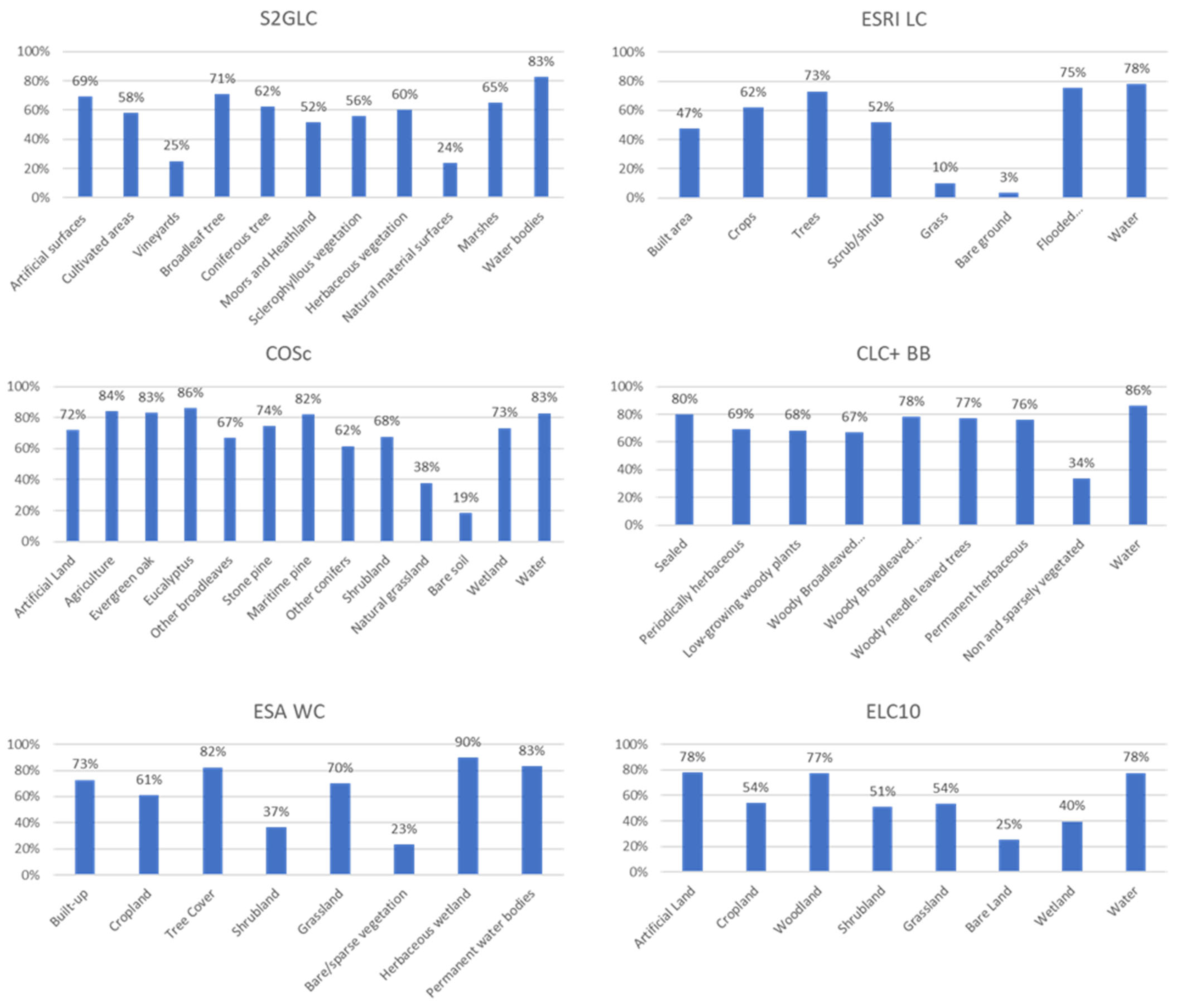
The accuracy results showed that all products had an overall accuracy between 51% and 72% when agreement between the map and reference database was considered, and whenever the map class was equal to the primary or secondary class identified in the reference database. If the agreement was only considered when the map equaled the primary class, the overall accuracy of the maps varied between 42% and 62%. In both situations, the maps with the highest overall accuracy were CLC+ BB and COSc, and the one with the least accuracy was ESRI LC. The F1-score values obtained for the classes of each product showed that there are classes in four of the six products analyzed with F1-score larger than 80% (one class in S2GLC, two in CLC+ BB, three in ESA WC and five in COSc), which means that the omission and commission errors were both small and therefore the class was very likely well represented in the map. In the same way, it is also clear that in all products there are classes mapped with low accuracy, which in most cases was the class “Bare land”.

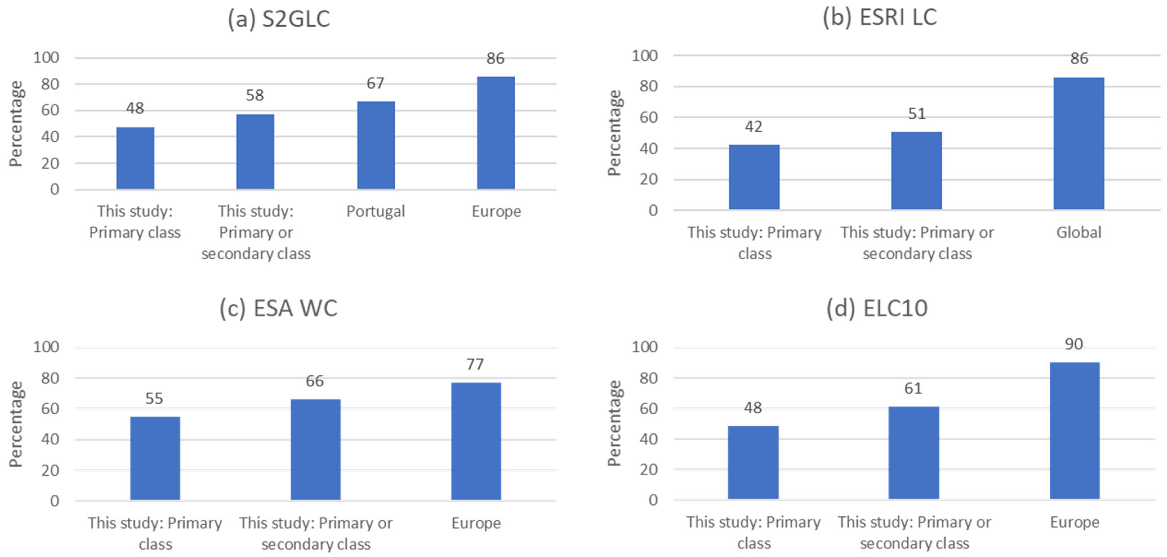
The overall accuracy values obtained in this study for the products were much lower than the accuracy values reported by the map producers for Portugal, Europe, and the globe, depending on what was made available by the producers. The values of per class user’s and producer’s accuracy varied even more for some classes in all products, which shows that for applications that have a particular interest in certain classes, their accuracy needs to be assessed in order to determine the fit for purpose of each map.

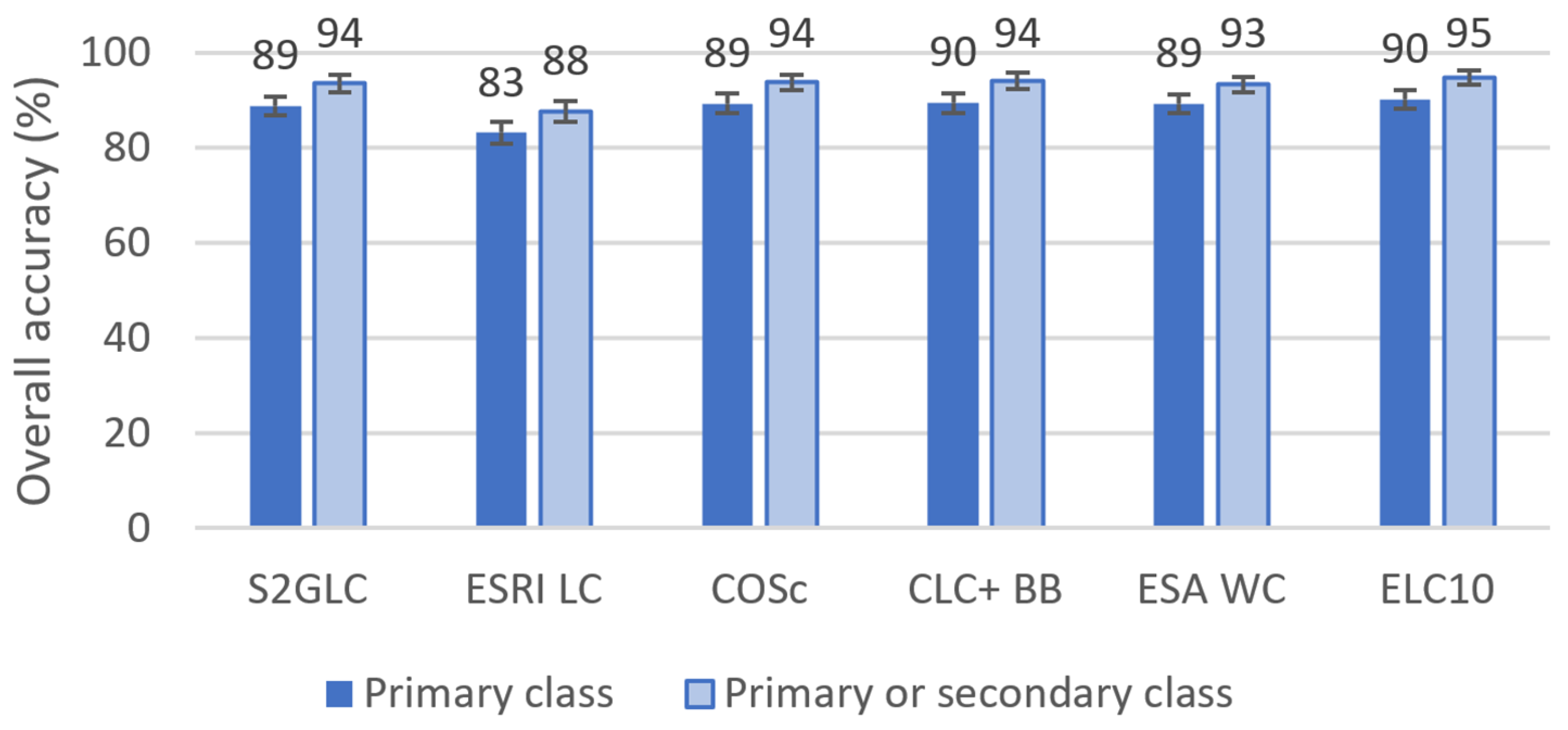
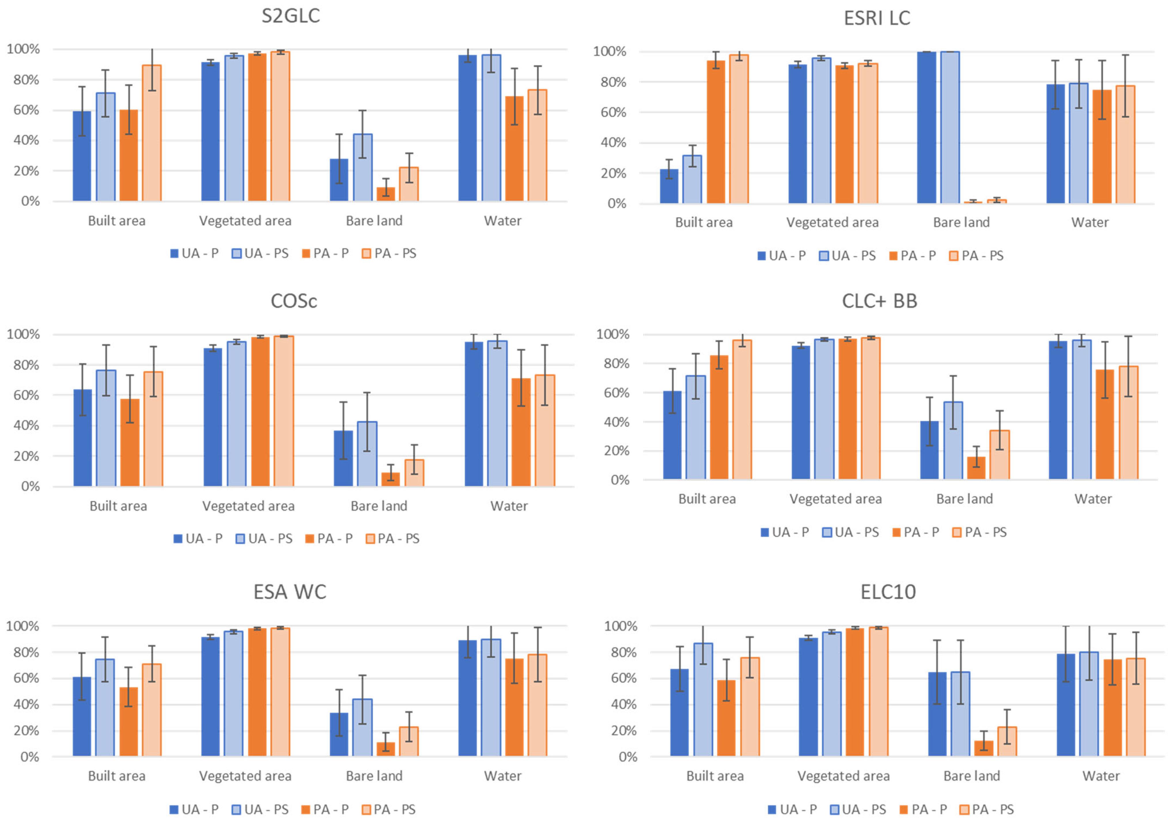
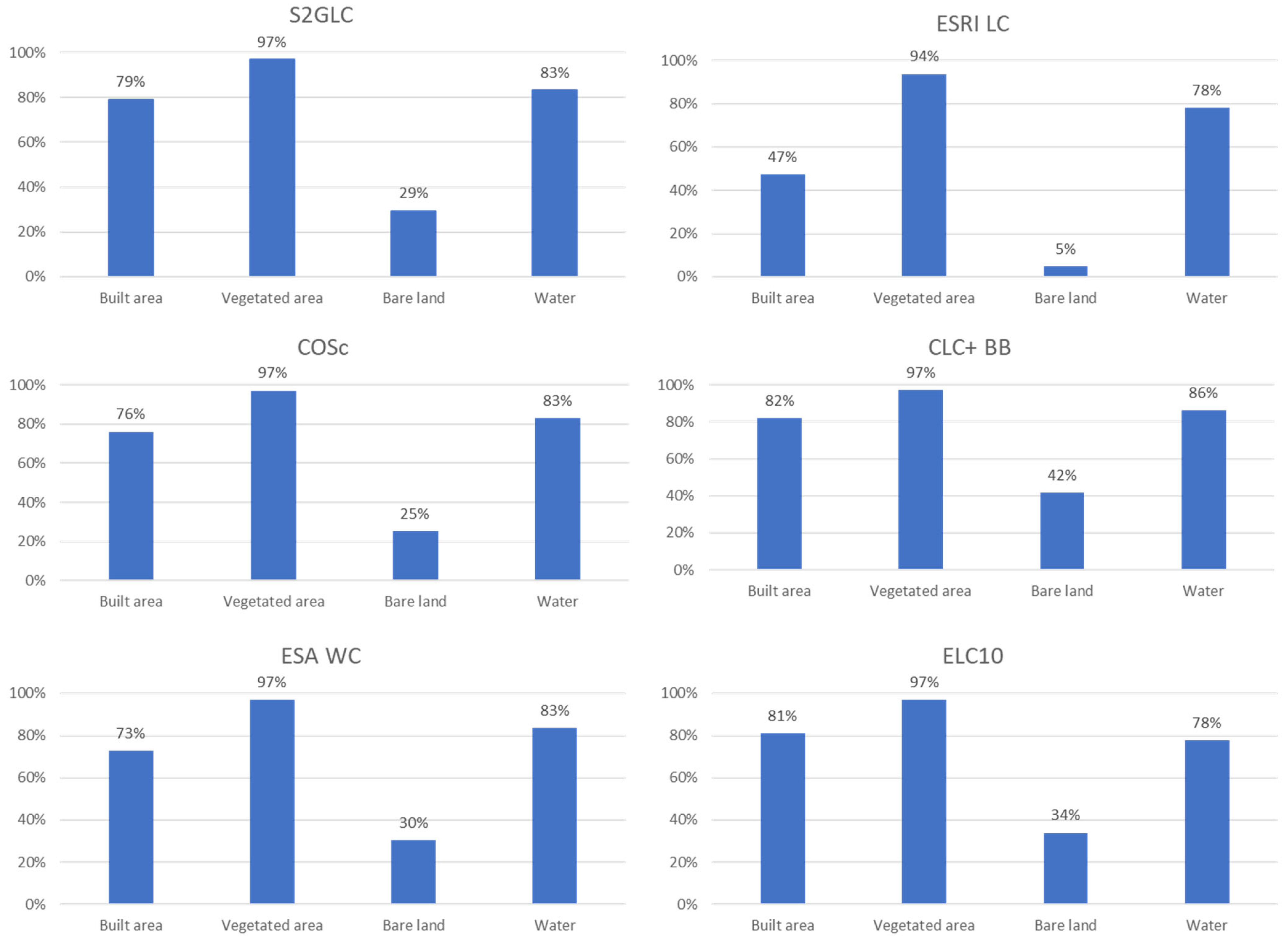
Since the products have different nomenclatures, a harmonization was made between all products into a four class HN: “Built area”, “Vegetated areas”, “Bare land” and “Water”. The overall accuracies of the harmonized products were higher, varying between 83% and 95%, depending on the original map and the methodology to assess the accuracy (see Figure 15). However, this is mainly due to the class “Vegetated areas”, which occupies most of the map, as there are very large differences in the user’s and producer’s accuracy for mainly “Built area” and “Bare land” classes. Nevertheless, it is important to stress that having fewer classes on a map does not imply superiority over maps with more detailed classes. While maps with fewer classes typically exhibit higher thematic quality, they lack the level of detail required for many applications. A direct comparison of the products regarding these four classes showed there are many important differences between the products, in terms of areas occupied by each class but also in terms of detail and feature’s continuity. The product showing more differences from the others was ESRI LC. The regions equally classified with all classes correspond to 83% of the study area. However, this region corresponds mostly to the class “Vegetated area”, while the large differences in the classes “Bare land” and “Built area” can be easily spotted.

The presented results show that the selection of a map to use for a particular application is not an easy task and the available products need to be assessed to determine which provide the necessary information. Methodologies that take into consideration the relative importance of different classes may also be used, to assess how each map may be fit for each application [55]. It is also relevant to point out that the production of global or European products is optimized to provide better results for the whole region to be mapped, which may imply that the mapping methodologies are not able to correctly map smaller regions with specific landscapes. Therefore, for demanding applications, even though European or global products are available, it may be necessary to generate local products, so that the specificities of the country’s landscapes are taken into consideration. This is in accordance with the fact that the accuracy results obtained with this analysis for Portugal were lower than the ones obtained for the European and global products, which is consistent with what has been found for other areas of the world.

The analysis performed within this paper stresses the importance of accuracy assessment. In fact, the obtained results may change if different approaches are used (both in terms of sampling strategy, response design, spatial representativeness, etc.), so it is important to use statistical best practices so that meaningful and reliable results are obtained for a specific need. On the other hand, validation is a resource consuming task. So, given the increasing number of maps made available every year, this topic is becoming more challenging, and new more automated approaches might need to be developed so that at least a preliminary estimation of the maps thematic accuracy may be obtained before a more thorough analysis can be performed.

References

1. Ren, W.; Tian, H.; Tao, B.; Yang, J.; Pan, S.; Cai, W.-J.; Lohrenz, S.E.; He, R.; Hopkinson, C.S. Large Increase in Dissolved Inorganic Carbon Flux from the Mississippi River to Gulf of Mexico Due to Climatic and Anthropogenic Changes over the 21st Century. J. Geophys. Res. Biogeosciences 2015, 120, 724–736. [Google Scholar] [CrossRef]
2. Li, Z.; Liu, S.; Tan, Z.; Sohl, T.L.; Wu, Y. Simulating the Effects of Management Practices on Cropland Soil Organic Carbon Changes in the Temperate Prairies Ecoregion of the United States from 1980 to 2012. Ecol. Model. 2017, 365, 68–79. [Google Scholar] [CrossRef]
3. Moiceanu, G.; Dinca, M.N. Climate Change-Greenhouse Gas Emissions Analysis and Forecast in Romania. Sustainability 2021, 13, 12186. [Google Scholar] [CrossRef]
4. Stevens, F.R.; Gaughan, A.E.; Linard, C.; Tatem, A.J. Disaggregating Census Data for Population Mapping Using Random Forests with Remotely-Sensed and Ancillary Data. PLoS ONE 2015, 10, e0107042. [Google Scholar] [CrossRef]
5. Schneider, A. Monitoring Land Cover Change in Urban and Peri-Urban Areas Using Dense Time Stacks of Landsat Satellite Data and a Data Mining Approach. Remote Sens. Environ. 2012, 124, 689–704. [Google Scholar] [CrossRef]
6. European Commission; Directorate-General for Communication. The European Green Deal; European Commission: Brussels, Belgium, 2020; ISBN 978-92-76-17190-4.
7. Naeem, S.; Cao, C.; Fatima, K.; Najmuddin, O.; Acharya, B.K. Landscape Greening Policies-Based Land Use/Land Cover Simulation for Beijing and Islamabad—An Implication of Sustainable Urban Ecosystems. Sustainability 2018, 10, 1049. [Google Scholar] [CrossRef]
8. Kidane, M.; Bezie, A.; Kesete, N.; Tolessa, T. The Impact of Land Use and Land Cover (LULC) Dynamics on Soil Erosion and Sediment Yield in Ethiopia. Heliyon 2019, 5, e02981. [Google Scholar] [CrossRef] [PubMed]
9. Cihlar, J. Land Cover Mapping of Large Areas from Satellites: Status and Research Priorities. Int. J. Remote Sens. 2000, 21, 1093–1114. [Google Scholar] [CrossRef]
10. Stehman, S.V.; Pengra, B.W.; Horton, J.A.; Wellington, D.F. Validation of the U.S. Geological Survey’s Land Change Monitoring, Assessment and Projection (LCMAP) Collection 1.0 Annual Land Cover Products 1985–2017. Remote Sens. Environ. 2021, 265, 112646. [Google Scholar] [CrossRef]
11. Jun, C.; Ban, Y.; Li, S. Open Access to Earth Land-Cover Map. Nature 2014, 514, 434. [Google Scholar] [CrossRef]
12. Gong, P.; Liu, H.; Zhang, M.; Li, C.; Wang, J.; Huang, H.; Clinton, N.; Ji, L.; Li, W.; Bai, Y.; et al. Stable Classification with Limited Sample: Transferring a 30-m Resolution Sample Set Collected in 2015 to Mapping 10-m Resolution Global Land Cover in 2017. Sci. Bull. 2019, 64, 370–373. [Google Scholar] [CrossRef] [PubMed]
13. Malinowski, R.; Lewiński, S.; Rybicki, M.; Gromny, E.; Jenerowicz, M.; Krupiński, M.; Nowakowski, A.; Wojtkowski, C.; Krupiński, M.; Krätzschmar, E.; et al. Automated Production of a Land Cover/Use Map of Europe Based on Sentinel-2 Imagery. Remote Sens. 2020, 12, 3523. [Google Scholar] [CrossRef]
14. Karra, K.; Kontgis, C.; Statman-Weil, Z.; Mazzariello, J.C.; Mathis, M.; Brumby, S.P. Global Land Use/Land Cover with Sentinel 2 and Deep Learning. In Proceedings of the 2021 IEEE International Geoscience and Remote Sensing Symposium IGARSS, Brussels, Belgium, 11–16 July 2021; pp. 4704–4707. [Google Scholar]
15. Venter, Z.S.; Sydenham, M.A.K. Continental-Scale Land Cover Mapping at 10 m Resolution Over Europe (ELC10). Remote Sens. 2021, 13, 2301. [Google Scholar] [CrossRef]
16. Zanaga, D.; Van De Kerchove, R.; De Keersmaecker, W.; Souverijns, N.; Brockmann, C.; Quast, R.; Wevers, J.; Grosu, A.; Paccini, A.; Vergnaud, S.; et al. ESA WorldCover 10 m; 2020 V100 2021; EAS: Paris, France, 2020.
17. ESA WorldCover. Product Validation Report, v1.1 2021; EAS: Paris, France, 2021.
18. Duarte, D.; Fonte, C.; Costa, H.; Caetano, M. Thematic Comparison between ESA WorldCover 2020 Land Cover Product and a National Land Use Land Cover Map. Land 2023, 12, 490. [Google Scholar] [CrossRef]
19. Chaaban, F.; El Khattabi, J.; Darwishe, H. Accuracy Assessment of ESA WorldCover 2020 and ESRI 2020 Land Cover Maps for a Region in Syria. J. Geovis. Spat. Anal. 2022, 6, 31. [Google Scholar] [CrossRef]
20. Stehman, S.V.; Wickham, J.D.; Smith, J.H.; Yang, L. Thematic Accuracy of the 1992 National Land-Cover Data for the Eastern United States: Statistical Methodology and Regional Results. Remote Sens. Environ. 2003, 86, 500–516. [Google Scholar] [CrossRef]
21. Wickham, J.; Stehman, S.V.; Gass, L.; Dewitz, J.A.; Sorenson, D.G.; Granneman, B.J.; Poss, R.V.; Baer, L.A. Thematic Accuracy Assessment of the 2011 National Land Cover Database (NLCD). Remote Sens. Environ. 2017, 191, 328–341. [Google Scholar] [CrossRef]
22. Wickham, J.; Stehman, S.V.; Sorenson, D.G.; Gass, L.; Dewitz, J.A. Thematic Accuracy Assessment of the NLCD 2016 Land Cover for the Conterminous United States. Remote Sens. Environ. 2021, 257, 112357. [Google Scholar] [CrossRef]
23. Wickham, J.; Stehman, S.V.; Sorenson, D.G.; Gass, L.; Dewitz, J.A. Thematic Accuracy Assessment of the NLCD 2019 Land Cover for the Conterminous United States. GIScience Remote Sens. 2023, 60, 2181143. [Google Scholar] [CrossRef]
24. Bie, Q.; Luo, J.; Lu, G. Accuracy Performance of Three 10-m Global Land Cover Products Around 2020 in an Arid Region of Northwestern China. IEEE Access 2023, 11, 133215–133228. [Google Scholar] [CrossRef]
25. Zhang, W.; Tian, J.; Zhang, X.; Cheng, J.; Yan, Y. Which Land Cover Product Provides the Most Accurate Land Use Land Cover Map of the Yellow River Basin? Front. Ecol. Evol. 2023, 11, 1275054. [Google Scholar] [CrossRef]
26. Venter, Z.S.; Barton, D.N.; Chakraborty, T.; Simensen, T.; Singh, G. Global 10 m Land Use Land Cover Datasets: A Comparison of Dynamic World, World Cover and Esri Land Cover. Remote Sens. 2022, 14, 4101. [Google Scholar] [CrossRef]
27. Zheng, K.; He, G.; Yin, R.; Wang, G.; Long, T. A Comparison of Seven Medium Resolution Impervious Surface Products on the Qinghai–Tibet Plateau, China from a User’s Perspective. Remote Sens. 2023, 15, 2366. [Google Scholar] [CrossRef]
28. Wang, Z.; Mountrakis, G. Accuracy Assessment of Eleven Medium Resolution Global and Regional Land Cover Land Use Products: A Case Study over the Conterminous United States. Remote Sens. 2023, 15, 3186. [Google Scholar] [CrossRef]
29. Stehman, S.V. Sampling Designs for Accuracy Assessment of Land Cover. Int. J. Remote Sens. 2009, 30, 5243–5272. [Google Scholar] [CrossRef]
30. Stehman, S.V. Estimating Area and Map Accuracy for Stratified Random Sampling When the Strata Are Different from the Map Classes. Int. J. Remote Sens. 2014, 35, 4923–4939. [Google Scholar] [CrossRef]
31. Moreira, F. Overview of Landscape Research and Assessment in Portugal. Belgeo 2004, 2–3, 329–336. [Google Scholar] [CrossRef]
32. Home | Global Land Cover—Sentinel 2. Available online: https://s2glc.cbk.waw.pl/ (accessed on 15 April 2024).
33. ESRI 2020 Land Cover. Available online: https://www.arcgis.com/home/item.html?id=d6642f8a4f6d4685a24ae2dc0c73d4ac (accessed on 31 March 2023).
34. Carta de Ocupação Do Solo Conjuntural—2020. Available online: https://dados.gov.pt/pt/datasets/carta-de-ocupacao-do-solo-conjuntural-2020/ (accessed on 31 March 2023).
35. Costa, H.; Benevides, P.; Moreira, F.D.; Moraes, D.; Caetano, M. Spatially Stratified and Multi-Stage Approach for National Land Cover Mapping Based on Sentinel-2 Data and Expert Knowledge. Remote Sens. 2022, 14, 1865. [Google Scholar] [CrossRef]
36. CLC+Backbone—Copernicus Land Monitoring Service. Available online: https://land.copernicus.eu/en/products/clc-backbone (accessed on 15 April 2024).
37. European Environment Agency. Technical Specifications for Implementation of a New Land-Monitoring Concept Based on EAGLE. D5: Design Concept and CLC+ Backbone, Technical Specifications, CLC+ Core and CLC+ Instances Draft Specifications, Including Requirements Review. Call for Tenders No EEA/DIS/R0/19/012—Annex 7—Version 5.4. 2019. Available online: https://www.google.com/url?sa=j&url=https%3A%2F%2Fetendering.ted.europa.eu%2Fdocument%2Fdocument-file-download.html%3FdocFileId%3D65292&uct=1705109396&usg=OBwu1DShixoRLIYDUdJ6oFwG0ac.&opi=89978449&ved=2ahUKEwit6I6YvtqFAxUZ7bsIHTL7A3wQwtwHKAB6BAgBEAE (accessed on 19 April 2024).
38. EAGLE Welcome Page—Copernicus Land Monitoring Service. Available online: https://land.copernicus.eu/eagle/welcome (accessed on 10 September 2021).
39. ESA WorldCover 2020. Available online: https://worldcover2020.esa.int/downloader (accessed on 31 March 2023).
40. Buchhorn, M.; Lesiv, M.; Tsendbazar, N.-E.; Herold, M.; Bertels, L.; Smets, B. Copernicus Global Land Cover Layers—Collection 2. Remote Sens. 2020, 12, 1044. [Google Scholar] [CrossRef]
41. COS 2018. Available online: https://geo2.dgterritorio.gov.pt/cos/COS2018/COS2018v2-gpkg.zip (accessed on 31 March 2023).
42. Direção Geral do Território, DGT Especificações Técnicas Da Carta de Uso e Ocupação Do Solo (COS) de Portugal Continental Para 2018; Direção Geral do Território: Lisbon, Portugal, 2019.
43. Stehman, S.V.; Foody, G.M. Key Issues in Rigorous Accuracy Assessment of Land Cover Products. Remote Sens. Environ. 2019, 231, 111199. [Google Scholar] [CrossRef]
44. Olofsson, P.; Foody, G.M.; Herold, M.; Stehman, S.V.; Woodcock, C.E.; Wulder, M.A. Good Practices for Estimating Area and Assessing Accuracy of Land Change. Remote Sens. Environ. 2014, 148, 42–57. [Google Scholar] [CrossRef]
45. Wagner, J.E.; Stehman, S.V. Optimizing Sample Size Allocation to Strata for Estimating Area and Map Accuracy. Remote Sens. Environ. 2015, 168, 126–133. [Google Scholar] [CrossRef]
46. Stehman, S.V.; Czaplewski, R.L. Design and Analysis for Thematic Map Accuracy Assessment: Fundamental Principles. Remote Sens. Environ. 1998, 64, 331–344. [Google Scholar] [CrossRef]
47. Manning, C.D.; Raghavan, P.; Schutze, H. An Introduction to Information Retrieval; Cambridge University Press: Cambridge, UK, 2009. [Google Scholar]
48. Liu, H.; Gong, P.; Wang, J.; Wang, X.; Ning, G.; Xu, B. Production of Global Daily Seamless Data Cubes and Quantification of Global Land Cover Change from 1985 to 2020—IMap World 1.0. Remote Sens. Environ. 2021, 258, 112364. [Google Scholar] [CrossRef]
49. García-Álvarez, D.; Lara Hinojosa, J.; Jurado Pérez, F.J.; Quintero Villaraso, J. Global General Land Use Cover Datasets with a Time Series of Maps. In Land Use Cover Datasets and Validation Tools: Validation Practices with QGIS; García-Álvarez, D., Camacho Olmedo, M.T., Paegelow, M., Mas, J.F., Eds.; Springer International Publishing: Cham, Switzerland, 2022; pp. 287–311. ISBN 978-3-030-90998-7. [Google Scholar]
50. Foody, G.M. Assessing the Accuracy of Land Cover Change with Imperfect Ground Reference Data. Remote Sens. Environ. 2010, 114, 2271–2285. [Google Scholar] [CrossRef]
51. Foody, G.M. Impacts of Ignorance on the Accuracy of Image Classification and Thematic Mapping. Remote Sens. Environ. 2021, 259, 112367. [Google Scholar] [CrossRef]
52. Sarmento, P.; Fonte, C.C.; Dinis, J.; Stehman, S.V.; Caetano, M. Assessing the Impacts of Human Uncertainty in the Accuracy Assessment of Land-Cover Maps Using Linguistic Scales and Fuzzy Intervals. Int. J. Remote Sens. 2015, 36, 2524–2547. [Google Scholar] [CrossRef]
53. Tsendbazar, N.; Herold, M.; Li, L.; Tarko, A.; de Bruin, S.; Masiliunas, D.; Lesiv, M.; Fritz, S.; Buchhorn, M.; Smets, B.; et al. Towards Operational Validation of Annual Global Land Cover Maps. Remote Sens. Environ. 2021, 266, 112686. [Google Scholar] [CrossRef]
54. Fonte, C.C.; See, L.; Laso-Bayas, J.C.; Lesiv, M.; Fritz, S. Assessing the Accuracy of Land Use Land Cover (LULC) Maps Using Class Proportions in The Reference Data. In ISPRS Annals of the Photogrammetry, Remote Sensing and Spatial Information Sciences; Copernicus GmbH: Göttingen, Germany, 2020; Volume V-3–2020, pp. 669–674. [Google Scholar]
55. Stehman, S.V. Comparing Thematic Maps Based on Map Value. Int. J. Remote Sens. 1999, 20, 2347–2366. [Google Scholar] [CrossRef]
Figure 1. Study area.
Remotesensing 16 01504 g001
Figure 2. LULC maps available for Portugal are compared and validated in this paper.
Remotesensing 16 01504 g002
Figure 3. Diagram of the methodology used to assess the accuracy and compare the six LULC maps.
Remotesensing 16 01504 g003
Figure 4. Illustration of the strata used in the sampling stage and the location of the sample points obtained through stratified random sampling.
Remotesensing 16 01504 g004
Figure 5. Examples where the choice of the reference class was performed differently: (a) the dominant class in the square cell (in blue) containing the sample point is with no doubt “Artificial Land”; (b) the cell containing the sample point includes “Permanent herbaceous” and “Woody broadleaved evergreen trees” in roughly equal proportions, so a primary and a secondary reference class were considered based on the cell surroundings.
Remotesensing 16 01504 g005
Figure 6. Overall accuracy of the original datasets considering there is an agreement between the reference dataset and the LULC maps when the primary class is the same (primary class) in both, or when either the primary or secondary class are the same (primary or secondary class). The black lines represent the 90% confidence intervals of the accuracy values.
Remotesensing 16 01504 g006
Figure 7. User’s (UA) and producer’s (PA) accuracy of the original products considering only the primary class (P) to assess the agreement between the reference data and the maps, and the primary or secondary class (PS). The black lines represent the 90% confidence intervals of the accuracy values.
Remotesensing 16 01504 g007
Figure 8. F1-score obtained for the classes of all products under analysis. These values enable to assess which products may provide high quality data for the several classes.
Remotesensing 16 01504 g008
Figure 9. Number of classes per product with F1-score in the five 20% equal range intervals.
Remotesensing 16 01504 g009
Figure 10. Comparison of the overall accuracy in this paper for S2GLC (a), ESRI LC (b), ESA WC (c) and ELC10 (d) with the results reported by map producers.
Remotesensing 16 01504 g010
Figure 11. User’s accuracy (UA) and producer’s accuracy (PA) per class of S2GLC computed with the reference database used in this paper considering only the primary class of the reference database to assess the agreement between the map and the reference data (UA—P and PA—P), considering the primary and secondary class (UA—PS and PA—PS), along with the results reported with the validation at the European level (UA—Europe and PA—Europe).
Remotesensing 16 01504 g011
Figure 12. User’s accuracy (UA) and producer’s accuracy (PA) per class of ESA WC computed with the reference database used in this paper considering only the primary class of the reference database to assess the agreement between the map and the reference data (UA—P and PA—P), or considering the primary and secondary class (UA—PS and PA—PS), along with the results obtained with the validation at the European level (UA—Europe and PA—Europe).
Remotesensing 16 01504 g012
Figure 13. User’s accuracy (UA) and producer’s accuracy (PA) per class of ELC10 computed with the reference database used in this paper considering only the primary class of the reference database to assess the agreement between the map and the reference data (UA—P and PA—P), or considering the primary and secondary class (UA—PS and PA—PS), along with the results obtained with the validation at the European level (UA—Europe and PA—Europe).
Remotesensing 16 01504 g013
Figure 14. User’s accuracy (UA) and producer’s accuracy (PA) per class of the ESRI LC computed with the reference database used in this paper considering only the primary class of the reference database to assess the agreement between the map and the reference data (UA—P and PA—P), or considering the primary and secondary class (UA—PS and PA—PS), along with the results obtained with global validation (UA—Global and PA—Global).
Remotesensing 16 01504 g014
Figure 15. Overall accuracy of the harmonized LULC maps, considering there is agreement between the reference dataset and the LULC maps when the primary class is the same (primary class) in both, or when either the primary or secondary class are the same (primary or secondary class). The black lines represent the 90% confidence intervals of the accuracy values.
Remotesensing 16 01504 g015
Figure 16. User’s (UA) and producer’s (PA) accuracy of the harmonized maps generated from each of the LULC original maps under analysis considering only the primary class (P) to assess the agreement between the reference data and the maps, and the primary or secondary class (PS). The black lines represent the 90% confidence intervals of the accuracy values.
Remotesensing 16 01504 g016
Figure 17. F1-score obtained for the maps derived from all products under analysis for the considered harmonized classes.
Remotesensing 16 01504 g017
Figure 18. Harmonized maps obtained with the mapping of the original nomenclature of each LULC product into the HN. The black rectangle shown in the maps corresponds to the detail shown in Figure 19.
Remotesensing 16 01504 g018
Figure 19. Harmonized maps corresponding to the black rectangle shown in Figure 18.
Remotesensing 16 01504 g019
Figure 20. 2018 orthorectified aerial images with 0.25 m spatial resolution of the region shown in Figure 19. The white ellipse corresponds to the region identified by the black ellipse in Figure 19.
Remotesensing 16 01504 g020
Figure 21. Detail of the region near the water body shown on the right lower part of Figure 19.
Remotesensing 16 01504 g021
Figure 22. Regions equally classified in all maps with the HN.
Remotesensing 16 01504 g022
Figure 23. Graph showing the area of each class in the harmonized maps derived from the six LULC maps, along with the area estimated from each map with the reference database using Equation (5).
Remotesensing 16 01504 g023