Maximum Likelihood Deconvolution of Beamforming Images with Signal-Dependent Speckle Fluctuations

Abstract

Ocean Acoustic Waveguide Remote Sensing (OAWRS) typically utilizes large-aperture linear arrays combined with coherent beamforming to estimate the spatial distribution of acoustic scattering echoes. The conventional maximum likelihood deconvolution (DCV) method uses a likelihood model that is inaccurate in the presence of multiple adjacent targets with significant intensity differences. In this study, we propose a deconvolution algorithm based on a modified likelihood model of beamformed intensities (M-DCV) for estimation of the spatial intensity distribution. The simulated annealing iterative scheme is used to obtain the maximum likelihood estimation. An approximate expression based on the generalized negative binomial (GNB) distribution is introduced to calculate the conditional probability distribution of the beamformed intensity. The deconvolution algorithm is further simplified with an approximate likelihood model (AM-DCV) that can reduce the computational complexity for each iteration. We employ a direct deconvolution method based on the Fourier transform to enhance the initial solution, thereby reducing the number of iterations required for convergence. The M-DCV and AM-DCV algorithms are validated using synthetic and experimental data, demonstrating a maximum improvement of 73% in angular resolution and a sidelobe suppression of 15 dB. Experimental examples demonstrate that the imaging performance of the deconvolution algorithm based on a linear small-aperture array consisting of 16 array elements is comparable to that obtained through conventional beamforming using a linear large-aperture array consisting of 96 array elements. The proposed algorithm is applicable for Ocean Acoustic Waveguide Remote Sensing (OAWRS) and other sensing applications using linear arrays.

1. Introduction

Horizontal coherent line arrays are commonly employed to capture scattered acoustic signals from diverse scatterers and sources in the undersea environment [1,2,3]. In a typical wide-area application, such as Ocean Acoustic Waveguide Remote Sensing (OAWRS), acoustic images are generated as a function of azimuthal angle and range using plane wave conventional beamforming (CBF) and travel time analysis to chart the spatial distribution of scatterers and sources, including fish aggregation [4,5], marine mammals [6,7], and seabed geographic features [8,9,10]. The direction of arrival (DOA) estimation performance of CBF is typically compromised due to its relatively wide beam width, which limits the capability to detect two targets that are close to each other. CBF is also generally considered a biased estimator of incident plane wave intensity, which is critical for discerning the temporal and spatial characteristics of the target. This estimation bias arises due to the inherent characteristics of CBF, particularly its sensitivity to the steering vector of the array and its susceptibility to the presence of noise and interference. CBF can non-linearly blur the angular distribution of incident plane wave intensities for array geometries that lack spherical symmetry. These limitations are particularly notable in scenarios where there are multiple sources and the array’s response is influenced by factors such as sidelobes and beam width.

Alternative techniques and algorithms, such as the minimum variance distortionless response (MVDR) [11] and multiple signal classification (MUSIC) algorithms [12], have been proposed based on the covariance matrix of array measurements to overcome the limitations of CBF on angular resolution and intensity estimation. Despite their utility in spatial signal processing, the MVDR and MUSIC algorithms face considerable limitations, including high sensitivity to interference [13] and a requirement for high signal-to-noise ratios to accurately identify signal directions or frequencies. Furthermore, the MUSIC algorithm is notably burdened by its computational intensity due to the necessity of eigendecomposition [14], posing challenges for real-time applications. Additionally, the effectiveness of these algorithms is contingent upon accurate prior knowledge regarding the number of signal sources [15] and precise array calibration [16]. These factors, if misestimated or erroneous, can lead to diminished accuracy in practical scenarios.

In recent years, compressed sensing (CS) theory [17] has been widely used in DOA estimation through solving the least squares problem while minimizing the ${\mathcal{l}}_1$ norm, which utilizes the sparsity of the number of sources in the data. Following the principles of compressed sensing, numerous outstanding algorithms have been proposed, including orthogonal matching pursuit (OMP) [18,19,20] and atomic norm minimizing [21,22,23]. These algorithms can significantly reduce the number of sensors to be used through exploiting the sparsity of the signal, as well as decreasing the number of samples required for signal restoration and bearing estimation. Although compressed sensing-based algorithms for DOA estimation generally exhibit strong robustness compared with other covariance matrix-based algorithms, their performance is significantly affected by the assumption of signal sparsity, which is commonly not applicable for OAWRS in imaging of large fish aggregation or extended geological features.

Essentially, the CBF output can be considered as the incident intensity signal modulated by the beam pattern, where the beam pattern can be regarded as the system function of the channel. The intensity distribution estimation of the incident signals can fundamentally be viewed as a deconvolution problem or a signal recovery issue. In the field of underwater acoustic communication, various methods have been proposed to address signal recovery or channel estimation problems in different scenarios. Common channel estimation methods include the least squares (LS) algorithm [24], the minimum mean square error (MMSE) algorithm [25], the time-reversal algorithm [26], and the compressed sensing algorithm [27]. An adaptive filtering algorithm [28] based on recursive least squares has recently been proposed, which reduces interference in channel estimation, providing higher accuracy and better interference cancellation effect. Additionally, deep learning methods [29,30,31] have been proposed for channel estimation without channel statistics information, mainly through learning complex underwater channel properties from the received signals.

A deconvolution approach based on the Richardson–Lucy (RL) algorithm originating from the field of image deblurring was recently proposed for high-resolution bearing estimation with a small-aperture linear array [32]. The algorithm generally deconvolves the intensity distribution of CBF output blurred by the beam pattern. It simultaneously provides narrow beam width and low sidelobes while retaining the advantages of robustness and less computation in CBF [33]. Although the algorithm has been widely used for image enhancement in optical applications [34,35,36], it does not estimate the real intensity of the original target, making it unsuitable for OAWRS and other acoustical wide-area applications.

An alternative deconvolution method (DCV) based on maximum likelihood (ML) estimation [37] has been developed, which provides satisfying performance regarding the estimation of the spatial intensity distribution of incident plane waves from the CBF output. The algorithm takes advantage of the relatively pervasive circular complex Gaussian random (CCGR) statistics of acoustic fields in the ocean that follow from the central limit theorem [38,39,40,41]. Based on the assumption that the CBF output intensity measured at a certain scan angle also follows a Gamma distribution [42], the ML estimator was derived to resolve the angular distribution of incident plane wave intensities from coherent array measurements. However, in the marine environment, the plane waves incident from adjacent directions typically have significant differences in intensity. The statistics of CBF output intensity measured at a certain scan angle deviate from the Gamma distribution, leading to a noticeable performance degradation.

In this study, we derive a deconvolution algorithm with a modified likelihood model (M-DCV) to estimate the spatial intensity distribution by deconvolving the CBF output. The beamformed intensity of one single incident plane wave measured at a certain scan angle is assumed to follow a Gamma distribution. The CBF output intensity measured at a certain scan angle is, hence, considered as the summation of multiple independent but not identical Gamma-distributed beamformed intensities. A computationally efficient approximate expression based on a generalized negative binomial (GNB) distribution is introduced to calculate the conditional probability distribution of the beamformed intensity. The simulated annealing iterative scheme [43] is employed to obtain the maximum likelihood estimation. This iterative approach necessitates recalculation of the conditional probability distribution of the beamforming output at each iteration step. To reduce the computational complexity of each iteration, we simplify the deconvolution algorithm with an approximate signal model (AM-DCV), which can significantly reduce the number of random signals that need to be considered when calculating the conditional probability distribution at each iteration. Moreover, a direct deconvolution method based on the Fourier transform is employed to enhance the initial solution in the iterative scheme, thereby reducing the number of iterations required. The deconvolution algorithm proposed in this study addresses the performance degradation issue of the conventional deconvolution (DCV) algorithm in the presence of multiple adjacent targets with significant intensity differences.

The M-DCV and AM-DCV algorithms offer several advantages compared with the existing approaches as follows.

(1)

The algorithms yield better angular resolution (up to 73%) and lower sidelobes (15 dB) compared with the CBF algorithm, depending on the width and incident angle of the features.

(2)

The algorithms retain the advantages of the CBF algorithm in terms of robustness and the number of snapshots required for processing.

(3)

The algorithms provide better estimation of intensity distribution compared with other deconvolution algorithms (DCV and RL), especially for targets close to the end-fire direction of the array.

(4)

The algorithms can significantly reduce the array aperture (~6 times smaller) and, at the same time, achieve performance outcomes comparable to those achieved using the CBF algorithm with large-aperture arrays.

These improvements were validated using both synthetic and experimental data.

2. Methods

2.1. Beamformed Complex Pressure Amplitude on a Discrete Receiver Array

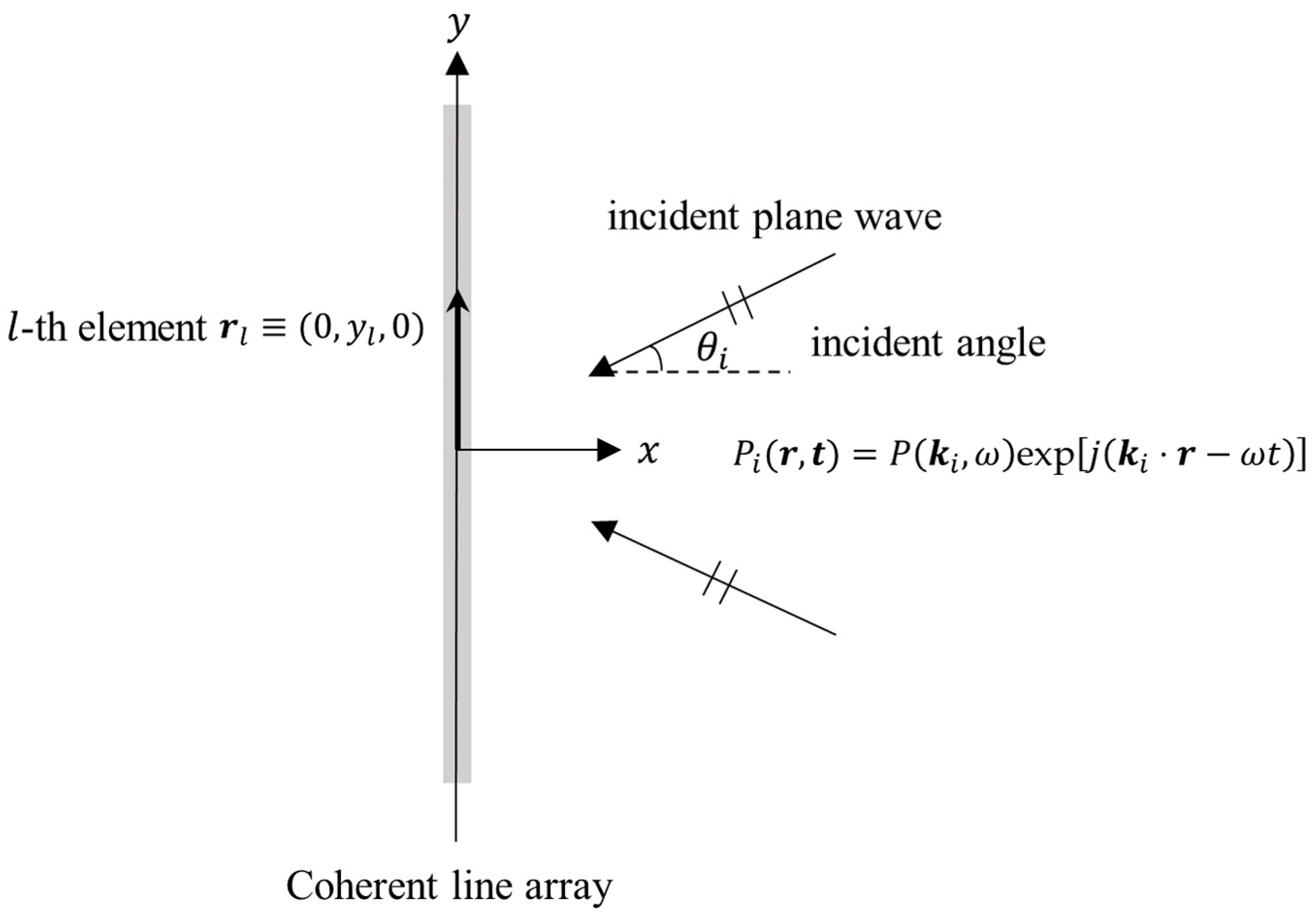
Let $P_i\left(\mathit{r},t\right)=P\left({\mathit{k}}_i,\omega \right)$exp$\left[j\left({\mathit{k}}_i\cdot \mathit{r}-\omega t\right)\right]$ denote the pressure field at spatial location $\mathit{r}$ and time $t$ due to a time-harmonic plane wave propagating in the direction of the acoustic wave number vector ${\mathit{k}}_i=k_x^i{\mathit{u}}_x+k_y^i{\mathit{u}}_y+k_z^i{\mathit{u}}_z$, where $\mathit{u}$ is the unit vector, $P\left({\mathit{k}}_i,\omega \right)$ is the complex amplitude,$k=\left|{\mathit{k}}_i\right|=\omega /c$ is the wavenumber vector, $\omega$ is the radial frequency, $c$ is the speed of sound, and $i$ is the index for $i=\mathrm{1,2},3\dots ,M$ directions. A uniformly spaced linear array of length $L$containing $N$ elements is aligned horizontally along the $y$-axis in the ocean waveguide with elements located at ${\mathit{r}}_l=(0,y_l,0)$, where $l$ $=1,2,...,N$ (Figure 1). A plane wave from any of the $M$ directions is incident on this discrete receiver array. The pressure field received on the $l$-th element of the array located at ${\mathit{r}}_l=(0,y_l,0)$ is $P_i\left({\mathit{r}}_l,t\right)=P\left({\mathit{k}}_i,\omega \right)\mathrm{e}\mathrm{x}\mathrm{p}\left[j\left(k\mathrm{s}\mathrm{i}\mathrm{n}{\phi }_i\mathrm{s}\mathrm{i}\mathrm{n}{\theta }_i{y}_l-\omega t\right)\right]$, where ${\phi }_i$ is the inclination angle and ${\theta }_i$ is the azimuthal angle.

Assuming the plane waves are incident along the horizontal surface as the inclination angle $\phi =\pi /2$, then the total pressure field of the plane waves on the whole array measured at scan angle $\theta$ after beamforming is as follows:

$$\begin{array}{c}{P}_B(\theta ,t,\omega )={\displaystyle \sum _{i=1}^M}{\displaystyle \sum _{l=1}^N}P\left({\mathit{k}}_i,\omega \right)\exp \left\{j\left[k{y}_l\left(\sin {\theta }_i-sin\theta \right)-\omega t\right]\right\}\\ ={\displaystyle \sum _{i=1}^M}P\left({\mathit{k}}_i,\omega \right)B\left(\mathrm{s}\mathrm{i}\mathrm{n}\theta -\mathrm{s}\mathrm{i}\mathrm{n}{\theta }_i,\omega \right)e^{-j\omega t}\end{array}$$

(1)

where $B\left(\sin \theta ,\omega \right)$ is the discrete linear array beam pattern. For a uniformly spaced array with $N$ elements and a total length of $L$ for $y_l$ between [−L/2, L/2], the array beam pattern is given [44] by the following expression:

$$B\left(\sin \theta ,\omega \right)=\sum _{l=1}^N\mathrm{e}\mathrm{x}\mathrm{p}\left(-j{ky}_l\sin \theta \right)=\frac{1}{N}\frac{\sin \left(\frac{k}{2}Nd\sin \theta \right)}{\sin \left(\frac{k}{2}d\sin \theta \right)}$$

(2)

where $d=L/(N-1)$ is the array element spacing and $\theta$ spans from $-\pi /2$ to $\pi /2$.

2.2. Modified Likelihood Model of Beamformed Intensity Given the Expected Incident Plane Wave Intensity

Assuming there are $J$ discrete scan angles, the beamformed intensity is measured at the $j$-th scan angle ${\theta }_j$, which can be written as follows:

$$W_j=W\left({\theta }_j,\omega \right)={\left|\sum _{i=1}^{M}P\left({\mathit{k}}_i,\omega \right)B\left(\sin {\theta }_j-\sin {\theta }_i,\omega \right)\right|}^2$$

(3)

where $j$ is an index for$j=\mathrm{1,2},3\dots ,J$ scan angles. It has been proposed that the CBF output intensity measured at a certain scan angle follows a Gamma distribution [37]. However, the statistics of CBF output deviate from the Gamma distribution in the presence of multiple plane waves with significant differences in intensity incident from adjacent directions. In this study, we propose a modified likelihood model that models the beamformed intensity $W_j$ at a certain scan angle as the summation of multiple intensity components given by the following expression:

$$W_j={\left|\sum _{i=1}^M{P}_i{B}_{ij}\right|}^2=\sum _{i=1}^M{\left|P_i{B}_{ij}\right|}^2+\sum _{i=1}^M\sum _{k=1,k\ne i}^M\left|{P_{i}P}_k{B}_{ij}{B}_{kj}\right|=\sum _{i=1}^M{W}_{ij}+\alpha$$

(4)

where $P_i=P\left({\mathit{k}}_i,\omega \right)$ are the complex pressure fields from $M$ incident directions, $B_{ij}=B\left(\sin {\theta }_j-\sin {\theta }_i,\omega \right)$, $W_{ij}={\left|P_i{B}_{ij}\right|}^2$ denotes the intensity component from the $i$-th incident plane wave after beamforming, and $\alpha$ denotes the cross term. For OAWRS applications, the beamformed intensity measurements are commonly averaged over the time of the pulse width after matched filtering, which is typically on the order of 10 ms. Within this period, the mean of the incident plane wave complex amplitude is approximately zero, making the cross term $\alpha$ in Equation (4) negligible.

According to the central limit theorem, the incident plane wave complex amplitude $P\left({\mathit{k}}_i,\omega \right)$ follows circular complex Gaussian random (CCGR) statistics; therefore, the mean $〈P\left({\mathit{k}}_i,\omega \right)〉$ is zero [40,41]$.$ It is assumed that distinct incident plane waves are statistically independent of each other, such that $〈P\left({\mathit{k}}_i,\omega \right)P^{\mathrm{*}}\left({\mathit{k}}_j,\omega \right)〉=〈P\left({\mathit{k}}_i,\omega \right)〉〈P^{\mathrm{*}}\left({\mathit{k}}_j,\omega \right)〉$ for $i\ne j$ [40,41]. $S\left({\mathit{k}}_i,\omega \right)$=$\langle {\left|\mathrm{P}\left({\mathit{k}}_{\mathrm{i}},\mathsf{\omega }\right)\right|}^2\rangle$ is the expected intensity of the incident plane wave. The expected beamformed intensity at scan angle ${\theta }_j$ is then given by the following expression:

$$\sigma \left({\theta }_j,\omega \right)=〈W\left({\theta }_j,\omega \right)〉=\sum _{i=1}^{M}S\left({\mathit{k}}_i,\omega \right){\left|B\left({\sin \theta }_j-\sin {\theta }_i,\omega \right)\right|}^2$$

(5)

It can be noticed from Equation (4) that the beamformed intensity $W_j$ measured at a certain scan angle is the summation of M independent but not identical random variables $W_{ij}$. The conditional probability distribution of the beamformed intensity component $W_{ij}$ given the expected intensity vector $\mathbf{S}$ containing $S_i=S\left({\mathit{k}}_{\mathit{i}},\omega \right)=〈P\left({\mathit{k}}_i,\omega \right)P^{\mathrm{*}}\left({\mathit{k}}_i,\omega \right)〉$ from all horizontal azimuths is given by the following expression [42,45]:

$$P\left(W_{ij}\right|\mathbf{S})=\frac{{\left[\frac{{\eta }_j}{{\sigma }_{ij}\left(\mathbf{S}\right)}\right]}^{{\eta }_j}{W}_{ij}^{{\eta }_j-1}\exp \left[-{\eta }_j\frac{W_{ij}}{{\sigma }_{ij}\left(\mathbf{S}\right)}\right]}{\mathsf{\Gamma }\left({\eta }_j\right)}$$

(6)

where ${\eta }_j$ is equal to the signal-to-noise ratio (SNR) ${〈W_j〉}^2/〈W_j^2〉-{〈W_j〉}^2$ [42,45], ${\sigma }_{ij}\left(\mathbf{S}\right)=S\left({\mathit{k}}_i,\omega \right){\left|B\left({\sin \theta }_j-\sin {\theta }_i,\omega \right)\right|}^2$ is the component of expected intensity from the i-th incident plane wave after beamforming, and $\mathsf{\Gamma }$ represents the Gamma function.

In general, the exact probability distribution of the summation of multiple independent Gamma-distributed random variables is quite complicated and does not admit a closed and simple form [46]. Thus far, various implementations of exact probability distributions have been proposed; however, these are all based on approximations, often of the numerical type [47,48,49,50]. Below, we provide a computationally efficient approximate expression [51] based on a generalized negative binomial (GNB) distribution as follows:

$$P\left(W_j|\mathbf{S}\right)=\sum _{k=0}^{\mathrm{\infty }}{w}_k\frac{{\left[\frac{{\eta }_j}{{{\sigma }_{ij}\left(\mathbf{S}\right)}_{\mathrm{m}\mathrm{i}\mathrm{n}}}\right]}^{\rho +k}{W}_{ij}^{\rho +k-1}\exp \left[-{\eta }_j\frac{W_{ij}}{{{\sigma }_{ij}\left(\mathbf{S}\right)}_{\mathrm{m}\mathrm{i}\mathrm{n}}}\right]}{\mathsf{\Gamma }\left(\rho +k\right)}$$

(7)

where $\rho$ = $M{\eta }_j$, $M$ is the number of incident plane waves, $k=\mathrm{0,1},2...,$ ${{\sigma }_{ij}\left(\mathbf{S}\right)}_{\mathrm{m}\mathrm{i}\mathrm{n}}$ is the minimum value of ${\sigma }_{ij}\left(\mathbf{S}\right)$, and $w_k$ is a three-parameter GNB given by the following probability function:

$$GNB(k;r,p,b)=\left\{\begin{array}{c}\frac{r}{r+bk}\left(\begin{array}{c}r+bk\\ k\end{array}\right)p^k(1-p{)}^{r+bk-k},k=\mathrm{0,1},2,\dots \\ 0,k\ge \mu ,r+b\mu <0\end{array}\right.$$

(8)

The parameters $p,b$, and $r$ are approximated by the following expression:

$$\left\{\begin{array}{c}p=1-\frac{A}{2}+\sqrt{\frac{A^2}{4}-1}\\ b=\frac{1}{p}\left[1-{\left(\frac{\mu (1-p)}{{\mu }_2}\right)}^{1/2}\right]\\ r=\mu \left(\frac{1-pb}{p}\right),\end{array}\right.$$

(9)

where $A=-2+{\left[\mu {\mu }_3-3{\mu }_2^2\right]}^2/\left(\mu {\mu }_2^3\right)$. The roots are real if and only if $A\ge 2$, i.e., if ${\left[\mu {\mu }_3-3{\mu }_2^2\right]}^2/\left(\mu {\mu }_2^3\right)\ge 4.$For $A<2$, we set $b=1$. The values of three parameters $\mu ,{\mu }_2$, and ${\mu }_3$ are given by the following expression:

$$\left\{\begin{array}{c}\mu ={\displaystyle \sum _{i=1}^M}\frac{{\sigma }_{ij}\left(\mathbf{S}\right)}{{{\sigma }_{ij}\left(\mathbf{S}\right)}_{\mathrm{m}\mathrm{i}\mathrm{n}}}(1-\frac{{{\sigma }_{ij}\left(\mathbf{S}\right)}_{\mathrm{m}\mathrm{i}\mathrm{n}}}{{\sigma }_{ij}\left(\mathit{S}\right)}){\eta }_j\\ {\mu }_2={\displaystyle \sum _{i=1}^M}{\left(\frac{{\sigma }_{ij}\left(\mathbf{S}\right)}{{{\sigma }_{ij}\left(\mathbf{S}\right)}_{\mathrm{m}\mathrm{i}\mathrm{n}}}\right)}^2(1-\frac{{{\sigma }_{ij}\left(\mathbf{S}\right)}_{\mathrm{m}\mathrm{i}\mathrm{n}}}{{\sigma }_{ij}\left(\mathbf{S}\right)}){\eta }_j\\ {\mu }_3={\displaystyle \sum _{i=1}^M}{\left(\frac{{\sigma }_{ij}\left(\mathbf{S}\right)}{{{\sigma }_{ij}\left(\mathbf{S}\right)}_{\mathrm{m}\mathrm{i}\mathrm{n}}}\right)}^3(1-\frac{{{\sigma }_{ij}\left(\mathbf{S}\right)}_{\mathrm{m}\mathrm{i}\mathrm{n}}}{{\sigma }_{ij}\left(\mathbf{S}\right)}){(2-\frac{{{\sigma }_{ij}\left(\mathbf{S}\right)}_{\mathrm{m}\mathrm{i}\mathrm{n}}}{{\sigma }_{ij}\left(\mathbf{S}\right)})\eta }_j\end{array}\right.$$

(10)

The provided expression can be utilized to numerically calculate the probability distribution of the summation of multiple Gamma-distributed random variables with large variability in scale parameters ${\sigma }_{ij}\left(\mathbf{S}\right)/{\eta }_j$, which is common in OAWRS imaging applications.

In the OWARS imaging system, distinct beams are statistically independent [40,41]. Therefore, the log-likelihood function for the beamformed intensity vector $\mathbf{W}={\left[W_1,\dots ,W_J\right]}^T$ from all horizontal azimuths given the expected intensity vector $\mathbf{S}$ is then as follows:

$$\ln P\left(\mathbf{W}|\mathbf{S}\right)=\sum _{j=1}^J\ln P\left({\mathbf{W}}_j\right|\mathbf{S})$$

(11)

The maximum likelihood estimate (MLE) $\widehat{\mathbf{S}}$ is determined as the log-likelihood function and attains its global maxima with the simulated annealing method below [43]:

$$\widehat{\mathbf{S}}=\arg \underset{\mathbf{S}}{\max }\ln P\left(\mathbf{W}|\mathbf{S}\right)$$

(12)

2.3. Approximate Likelihood Model of Beamformed Intensity Given the Expected Incident Plane Wave Intensity

The modified likelihood model requires sequential convolution to compute the exact conditional probability distribution of the beamformed intensity measured at a certain scan angle, which leads to computationally expensive calculations. In this section, we propose an approximate likelihood model for reducing computational complexity.

The plane waves incident from different directions can be distinguished into effective signals and ambient noise based on a predefined threshold determined by the majority of incident plane waves with lower intensities. The expected incident plane wave intensity vector $\mathbf{S}={\left[S_1,S_2,\dots S_M\right]}^T$ can then be expressed as the summation of the effective signal intensity vector ${\mathbf{S}}_{\mathrm{s}\mathrm{i}\mathrm{g}}$ and the ambient noise intensity vector ${\mathbf{S}}_{\mathrm{n}\mathrm{o}\mathrm{i}\mathrm{s}\mathrm{e}}$:

$$\mathbf{S}={\mathbf{S}}_{\mathrm{s}\mathrm{i}\mathrm{g}}+{\mathbf{S}}_{\mathrm{n}\mathrm{o}\mathrm{i}\mathrm{s}\mathrm{e}}$$

(13)

The intensity vector ${\mathbf{S}}_{\mathrm{s}\mathrm{i}\mathrm{g}}$ contains the effective signal intensities $S_q=〈P\left({\mathit{k}}_q,\omega \right)P^{*}\left({\mathit{k}}_q,\omega \right)〉$ incident from $Q$ out of $M$ horizontal azimuths, and 0 in other $M-Q$ horizontal azimuths, where $q$ is an index for $q=\mathrm{1,2},3\dots ,Q$ and $P\left({\mathit{k}}_q,\omega \right)$ denotes the complex amplitude of the $q$-th effective signal. The intensity vector ${\mathbf{S}}_{\mathrm{n}\mathrm{o}\mathrm{i}\mathrm{s}\mathrm{e}}$ contains ambient noise intensities $S_i=〈P\left({\mathit{k}}_i,\omega \right)P^{*}\left({\mathit{k}}_i,\omega \right)〉$ incident from $M-Q$ horizontal azimuths, and 0 in other $Q$ horizontal azimuths, where $i$ is an index for $i=\mathrm{1,2},3\dots ,M-Q$ horizontal azimuths and $P\left({\mathit{k}}_i,\omega \right)$ denotes the complex amplitude of the $i$-th ambient noise.

The beamformed intensity $W_j$ measured at scan angle ${\theta }_j$ can then be written as the following expression:

$$W_j=W_{j,\mathrm{s}\mathrm{i}\mathrm{g}}+W_{j,\mathrm{n}\mathrm{o}\mathrm{i}\mathrm{s}\mathrm{e}}=\sum _{q=1}^Q{W}_{qj,\mathrm{s}\mathrm{i}\mathrm{g}}+W_{j,\mathrm{n}\mathrm{o}\mathrm{i}\mathrm{s}\mathrm{e}}$$

(14)

where $W_{j,\mathrm{s}\mathrm{i}\mathrm{g}}$ and $W_{j,\mathrm{n}\mathrm{o}\mathrm{i}\mathrm{s}\mathrm{e}}$ are the beamformed intensities of effective signals and ambient noise measured at scan angle ${\theta }_j$, and $W_{qj,\mathrm{s}\mathrm{i}\mathrm{g}}={\left|{P\left({\mathit{k}}_q,\omega \right)B}_{qj}\right|}^2$ denotes the intensity component from the $q$-th effective signal after beamforming.

The ambient noise in the marine environment can generally be approximated as omnidirectional in $M$ horizontal azimuths and uniform in intensity. Therefore, the ambient noise intensity vector ${\mathbf{S}}_{\mathrm{n}\mathrm{o}\mathrm{i}\mathrm{s}\mathrm{e}}$ can be approximated as a unit vector multiplied by the average intensity $\overline{S}$. Based on the above assumption, the expected beamformed intensity of ambient noise ${\sigma }_j\left({\mathbf{S}}_{\mathrm{n}\mathrm{o}\mathrm{i}\mathrm{s}\mathrm{e}}\right)$ measured at scan angle ${\theta }_j$ can be expressed as follows:

$${\sigma }_j\left({\mathbf{S}}_{\mathrm{n}\mathrm{o}\mathrm{i}\mathrm{s}\mathrm{e}}\right)=\sum _{i=1}^M\overline{S}{\left|B\left({\sin \theta }_j-\sin {\theta }_i,\omega \right)\right|}^2$$

(15)

where the ambient noise intensity vector ${\mathbf{S}}_{\mathrm{n}\mathrm{o}\mathrm{i}\mathrm{s}\mathrm{e}}$ and the average value of ambient noise intensity $\overline{S}$ can be obtained from the elements of the expected incident plane wave intensity vector $\mathbf{S}$ that are below the threshold. The conditional probability distribution of the beamformed intensity of ambient noise $P\left(W_{j,\mathrm{n}\mathrm{o}\mathrm{i}\mathrm{s}\mathrm{e}}|\mathbf{S}\right)$ given the expected incident plane wave intensity vector $\mathbf{S}$ at scan angle ${\theta }_j$ approximately obeys a Gamma distribution given by the following expression:

$$P\left(W_{j,\mathrm{n}\mathrm{o}\mathrm{i}\mathrm{s}\mathrm{e}}|\mathbf{S}\right)=\frac{{\left[\frac{{\eta }_j}{{\sigma }_j\left({\mathbf{S}}_{\mathrm{n}\mathrm{o}\mathrm{i}\mathrm{s}\mathrm{e}}\right)}\right]}^{{\eta }_j}{W}_{j,\mathrm{n}\mathrm{o}\mathrm{i}\mathrm{s}\mathrm{e}}^{{\eta }_j-1}\exp \left[-{\eta }_j\frac{W_{j,\mathrm{n}\mathrm{o}\mathrm{i}\mathrm{s}\mathrm{e}}}{{\sigma }_j\left({\mathbf{S}}_{\mathrm{n}\mathrm{o}\mathrm{i}\mathrm{s}\mathrm{e}}\right)}\right]}{\mathsf{\Gamma }\left({\eta }_j\right)}$$

(16)

where ${\sigma }_j\left({\mathbf{S}}_{\mathrm{n}\mathrm{o}\mathrm{i}\mathrm{s}\mathrm{e}}\right)$ and ${\eta }_j$ are only related to the normalized ambient noise level and scan angle, respectively.

The expected beamformed intensity of effective signals ${\sigma }_j\left({\mathbf{S}}_{\mathrm{s}\mathrm{i}\mathrm{g}}\right)$ measured at scan angle ${\theta }_j$ can be expressed as follows:

$${\sigma }_j\left({\mathbf{S}}_{\mathrm{s}\mathrm{i}\mathrm{g}}\right)=\sum _{q=1}^Q{S}_q{\left|B\left({\sin \theta }_j-\sin {\theta }_q,\omega \right)\right|}^2$$

(17)

where the effective signal intensity vector ${\mathbf{S}}_{\mathrm{s}\mathrm{i}\mathrm{g}}$ can be obtained from the elements of the expected incident plane wave intensity vector $\mathbf{S}$ that are above the threshold. Similar to Equation (4), the beamformed intensities of effective signals measured at the $j$-th scan angle $W_{j,\mathrm{s}\mathrm{i}\mathrm{g}}$ can be considered as the sum of $Q$ independent but not identical random variables $W_{qj,\mathrm{s}\mathrm{i}\mathrm{g}}$. The conditional probability distribution of the beamformed intensity components $W_{qj,\mathrm{s}\mathrm{i}\mathrm{g}}$ follows the Gamma statistics given by the following expression:

$$P\left(W_{qj,\mathrm{s}\mathrm{i}\mathrm{g}}|\mathbf{S}\right)=\frac{{\left[\frac{{\eta }_j}{{\sigma }_j\left({\mathbf{S}}_{\mathrm{s}\mathrm{i}\mathrm{g}}\right)}\right]}^{{\eta }_j}{W}_{qj,\mathrm{s}\mathrm{i}\mathrm{g}}^{{\eta }_j-1}\exp \left[-{\eta }_j\frac{W_{qj,\mathrm{s}\mathrm{i}\mathrm{g}}}{{\sigma }_j\left({\mathbf{S}}_{\mathrm{s}\mathrm{i}\mathrm{g}}\right)}\right]}{\mathsf{\Gamma }\left({\eta }_j\right)}$$

(18)

Therefore, the conditional probability distribution of the beamformed effective signal intensities $P\left(W_{j,\mathrm{s}\mathrm{i}\mathrm{g}}|\mathbf{S}\right)$ given the expected incident plane wave intensity vector $\mathbf{S}$ at scan angle ${\theta }_j$ can then be calculated using the approximate expression proposed in Section 2.2.

It should be noted that, in most OAWRS applications, effective signals are sparsely distributed in space (i.e., $Q\ll M$). Therefore, much fewer random variables need to be considered in the calculation of the conditional probability distribution of beamformed effective signals, which can significantly reduce the calculation complexity of the approximate expression.

It is assumed that the beamformed measurements of effective signals and ambient noise are statistically independent of each other. The conditional probability distribution of the beamformed intensity at scan angle ${\theta }_j$ can then be calculated as follows:

$$P\left(W_j|\mathbf{S}\right)=P\left(W_{j,\mathrm{n}\mathrm{o}\mathrm{i}\mathrm{s}\mathrm{e}}|\mathbf{S}\right)\ast P\left(W_{j,\mathrm{s}\mathrm{i}\mathrm{g}}|\mathbf{S}\right)$$

(19)

The maximum likelihood estimate $\widehat{\mathbf{S}}$ is obtained as the log-likelihood function which attains its global maxima with the simulated annealing method following Equation (11). We set a predefined threshold to separate the CBF output into effective signals and ambient noise. The initial value of $\overline{S}$ is determined as the average value of the CBF output below the threshold. The initial values of effective signal intensities are determined as the CBF output but are assumed to be zero at directions where the CBF output is smaller than the threshold. In the iteration process, effective signal intensity below the threshold at any scan angle is considered ambient noise.

2.4. Improvement in the Initial Intensity Distribution for Maximum Likelihood Estimation

The selection of the initial solution for the iterative process can significantly affect the convergence and efficiency of the ML deconvolution algorithm. Generally, we use the normalized CBF output as the initial solution vector [37]. However, for arrays with small apertures, CBF output deviates significantly from the ground truth distribution of incident plane wave intensity, which can greatly increase the number of iterations before convergence. Therefore, we propose a method to improve the initial solution vector by directly deconvolving the CBF output based on the Fourier transform technique.

According to Equation (5), the expected beamformed intensity $\sigma (\sin \theta ,\omega )$ can also be written as the convolution of the magnitude squared beam pattern $\mathbb{B}\left(\sin \theta ,\omega \right)={\left|B\left(\sin \theta ,\omega \right)\right|}^2$ with the expected incident plane wave intensity distribution $S\left(\sin {\theta }_i,\omega \right)$:

$$\begin{array}{c}\sigma \left(\sin \theta ,\omega \right)={\displaystyle \sum _{i=1}^M}S\left(\sin {\theta }_i,\omega \right){\left|B\left(\sin \theta -\sin {\theta }_i,\omega \right)\right|}^2\\ =S\left(\sin \theta ,\omega \right)\ast B\left(\sin \theta ,\omega \right)\end{array}$$

(20)

where $\ast$ denotes the convolution symbol. It can also be expressed in the wavenumber domain as the following expression:

$$\mathsf{\Sigma }\left(k\right)=S\left(k\right)·\mathbb{B}\left(k\right)$$

(21)

where $\mathsf{\Sigma }\left(k\right)$,$S\left(k\right)$, and $\mathbb{B}\left(k\right)$ are the Fourier transform values of $\sigma \left(\sin \theta ,\omega \right)$, $S\left(\sin \theta ,\omega \right)$, and $\mathbb{B}\left(\sin \theta ,\omega \right)$ in the wavenumber domain, respectively. In practical applications, $\mathsf{\Sigma }\left(k\right)$ is averaged over the beamforming measurements of multiple snapshots. According to Equation (21), the initial intensity distribution $S\left(k\right)$ in the wavenumber domain can be calculated as follows:

$$S\left(k\right)=\frac{\mathsf{\Sigma }\left(k\right)}{\mathbb{B}\left(k\right)}$$

(22)

Knowing the beam pattern of a given array, we can obtain the improved initial intensity distribution in the spatial domain using the inverse Fourier transform. The improved initial intensity distribution is more computationally effective for the simulated annealing iterative scheme.

3. Illustrative Examples

In this section, we first demonstrate the method proposed in Section 2.3 for computing the conditional probability distribution of CBF output of ambient noise in the approximate likelihood model. We use both simulated data from field experiments and real wide-area OAWRS data to validate the M-DCV and AM-DCV algorithms. We compare the reconstructed images obtained from the deconvolution algorithm with the true images to evaluate the performance and accuracy of the algorithm. The approximate expression in Section 2.2 is used to numerically calculate the conditional probability distribution, which is also the likelihood of beamformed intensity. We employ the simulated annealing iterative scheme to obtain the maximum likelihood estimation; this method helps us to extract the intensity distribution estimation from CBF outputs through iteratively updating the parameters to maximize the likelihood estimation. For the iterative process, the initial intensity distribution is calculated using the direct deconvolution method discussed in Section 2.4 for both the M-DCV and AM-DCV algorithms. This initial estimation serves as a starting point for the iterative refinement process.

3.1. Conditional Probability Distribution of Conventional Beamforming Output of the Ambient Noise

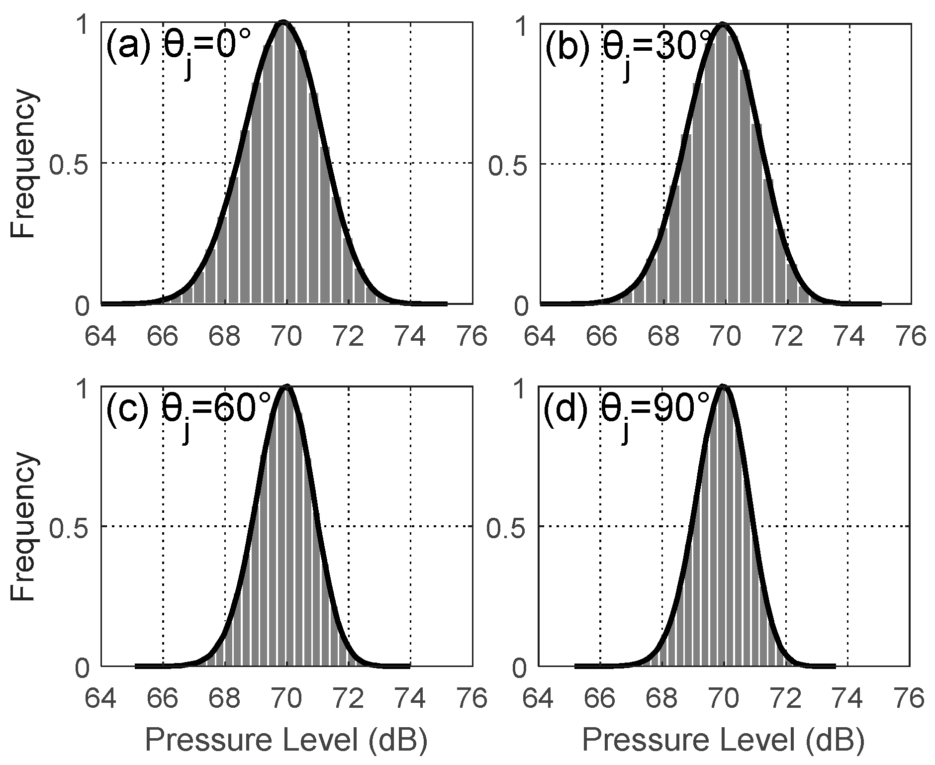
In this section, we first validate whether the conditional probability distribution of the CBF output of ambient noise $W_{j,\mathrm{n}\mathrm{o}\mathrm{i}\mathrm{s}\mathrm{e}}$ at one single scan angle approximately obeys the Gamma distribution $\mathsf{\Gamma }({\eta }_j,\frac{{\sigma }_j\left({\mathbf{S}}_{\mathrm{n}\mathrm{o}\mathrm{i}\mathrm{s}\mathrm{e}}\right)}{{\eta }_j})$. The Kolmogorov–Smirnov test is used to verify whether the conditional probability distribution follows a Gamma distribution. Through performing this validation, we can determine whether the method for computing the conditional probability distribution in the approximate likelihood model is accurate. This validation step is crucial as it ensures the reliability and correctness of the subsequent deconvolution algorithms.

We assume that the ambient noise level ${\mathbf{S}}_{\mathrm{n}\mathrm{o}\mathrm{i}\mathrm{s}\mathrm{e}}$ is 70 dB. The array is set as a uniform linear array consisting of 32 elements, and the element spacing is half of the plane wavelength. The speed of sound in water is $c=1500$ m/s.

As shown in Figure 2, we use the Monte Carlo method to calculate statistical histograms of the normalized CBF outputs at scan angles ${\theta }_j=$0°, 30°, 60°, and 90°, respectively. It is shown, in the figure, that the conditional probability distribution of ambient noise after CBF can be well-described using Gamma distributions (black line) with the proper scan angle-dependent shape parameters ${\eta }_j=\eta \left({\theta }_j\right)$. The scale parameter of the Gamma distribution can be automatically determined by the shape parameter ${\eta }_j$ and the expected beamformed intensity of ambient noise ${\sigma }_j\left({\mathbf{S}}_{\mathrm{n}\mathrm{o}\mathrm{i}\mathrm{s}\mathrm{e}}\right)$. The shape parameter ${\eta }_j$ as a function of scan angles is shown in Figure 3.

3.2. Simulation Data Results

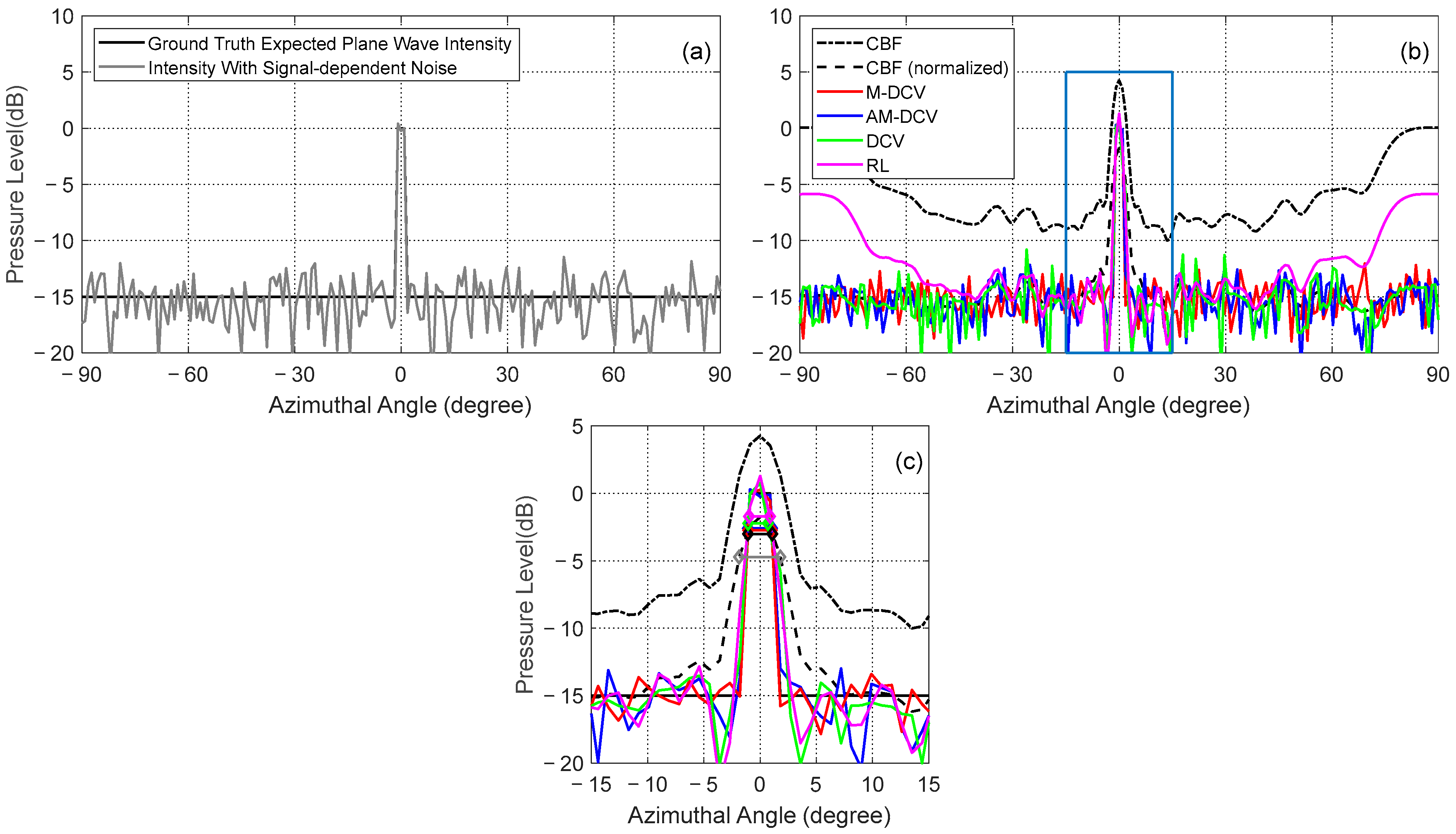
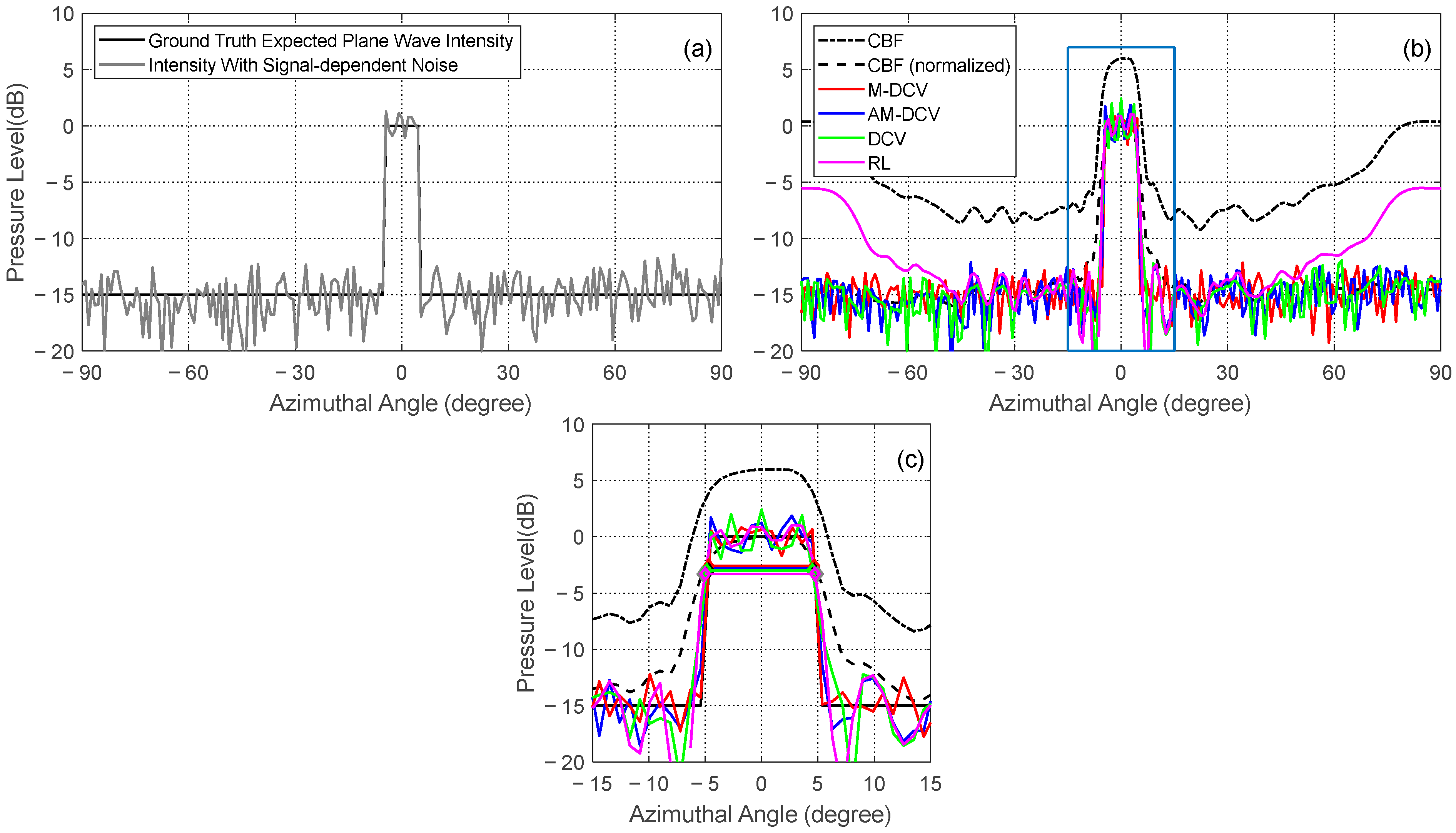
In this section, we demonstrate the deconvolution of incident CCGR fields using simulated data. The uniform linear receiver array consists of 32 elements, and the element spacing is half of the plane wavelength for all of the illustrations shown in this section. The speed of sound in water is $c=$ 1500 m/s. In Figure 4, Figure 5, Figure 6 and Figure 7 it is shown that, after using the M-DCV and AM-DCV algorithms, the angular resolution can be improved by a factor of 6–73%, depending on the width and incident angle of the features. The results of the DCV and RL algorithms are provided for comparison.

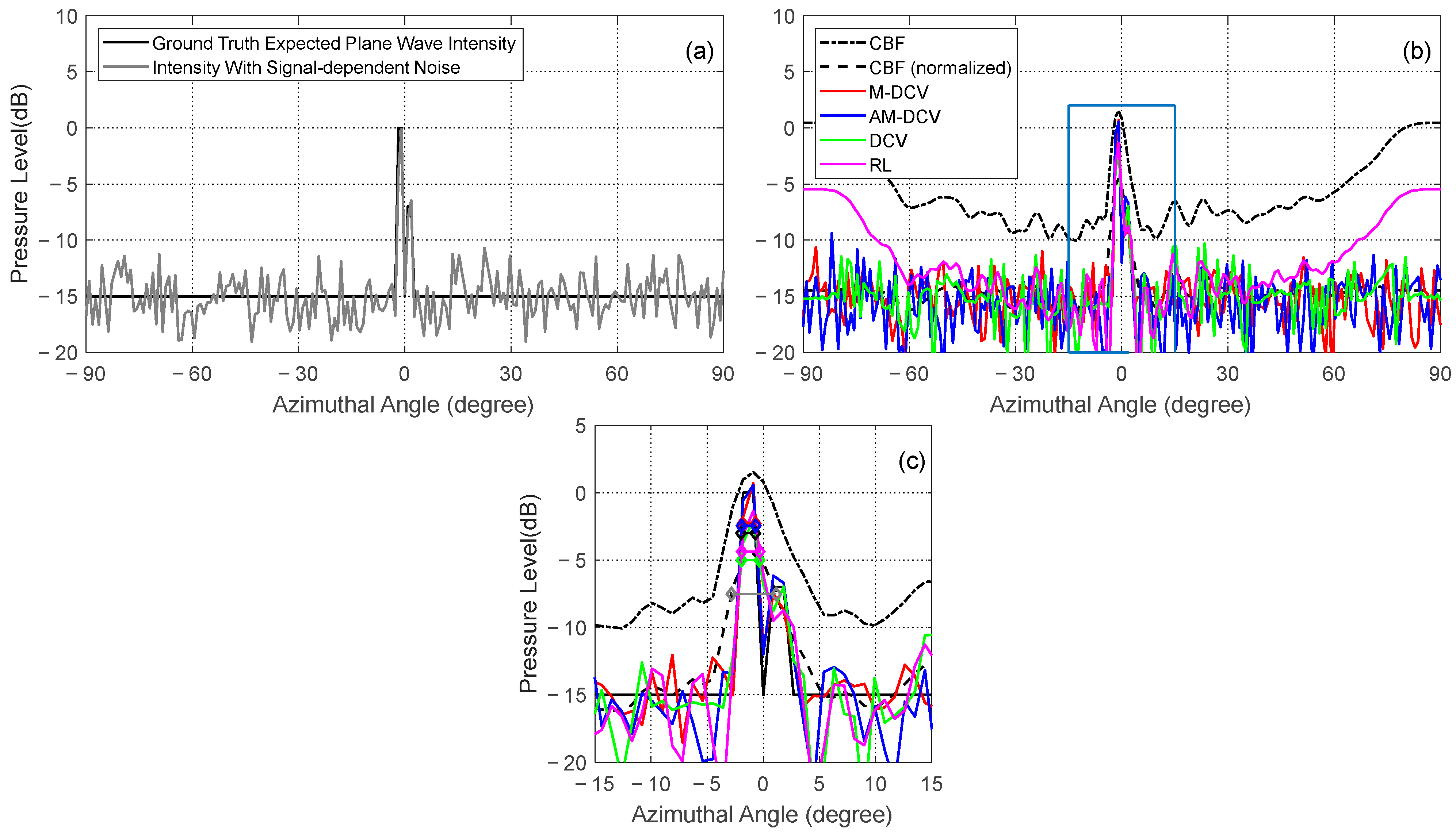
For a relatively narrow angular rectangle feature of 2° width at the array broadside, the 3 dB beam width values of the M-DCV, AM-DCV, DCV, and RL results are 2.12°, 2.21°, 1.86°, and 1.76°, respectively (Figure 4). This provides a maximum 42% improvement compared with CBF, which results in an output of 3.68°. For a relatively wide angular rectangle feature of 9° width at the array broadside, the 3 dB beam width of the M-DCV, AM-DCV, DCV, and RL results are 9.42°, 9.52°, 9.38°, and 9.72°, respectively (Figure 5). Compared with the CBF output with a 3 dB beam width of 10.02°, a maximum 6% angular resolution improvement is provided. In summary, the four algorithms all provide a narrow main lobe and low sidelobes. Additionally, the RL algorithm shows a significant deviation in the intensity distribution estimation near the end-fire direction of the array.

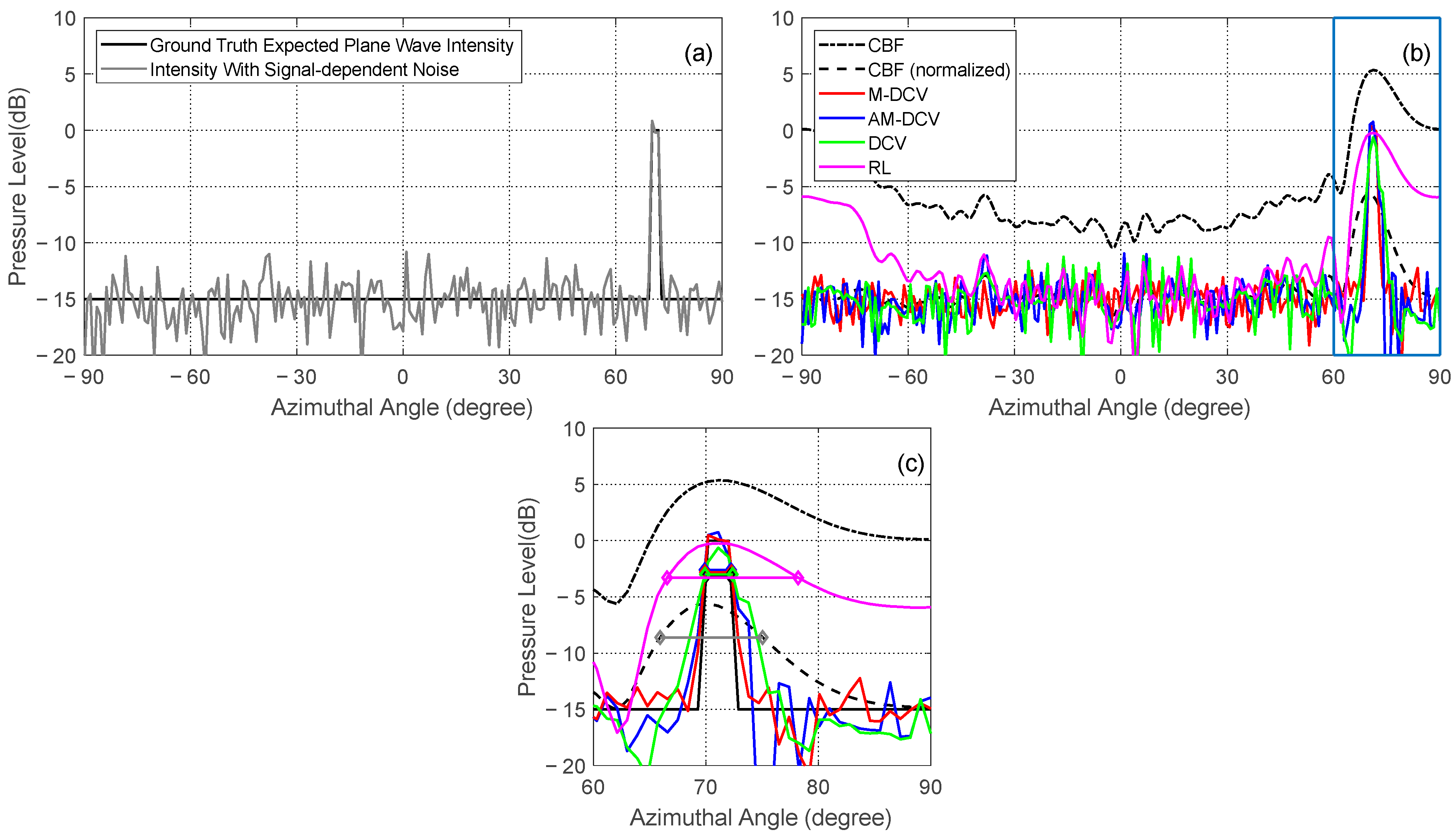
Next, we calculate the ML deconvolved estimate results for the same features; however, this set of features is located at the end-fire direction of the array, as shown in Figure 6 and Figure 7. For the relatively narrow angular rectangle feature, the 3 dB beam widths of the M-DCV, AM-DCV, DCV, and RL results are 2.40°, 2.46°, 2.45°, and 11.65°, respectively (Figure 6). A maximum 73% angular resolution improvement is provided, compared with that of the CBF output of 9.08°. For the relatively wide angular rectangle feature, the 3 dB beam widths of the M-DCV, AM-DCV, DCV, and RL results are 9.69°, 9.95°, 9.87°, and 17.06°, respectively (Figure 7). For comparison, the 3 dB beam width after CBF is 11.36°, and a maximum 15% improvement in angular resolution is provided. Compared with the DCV algorithm, the M-DCV and AM-DCV algorithms provide lower sidelobes while maintaining the resolution of the main lobe. Meanwhile, the 3 dB beam width of the RL results significantly increases as the scan angle approaches the end-fire direction, and its intensity estimation results are less accurate compared with other methods.

It can be noticed that the M-DCV and AM-DCV results maintain good angular resolution and intensity distribution estimation at both the broadside and end-fire directions of the array. The results also match the ground truth intensity better, when compared with the CBF output, which can help to reconstruct the fine distribution of the incident features. For the relatively narrow angular rectangle feature at the array broadside (Figure 4), the M-DCV result deteriorates the ground truth intensity at up to 15 dB down from the peak value, compared with that of CBF output at roughly 2 dB down from the peak value. The agreements between the M-DCV results and the ground truth intensities only deviate by no less than 7 dB down from the peak intensity, depending on the incident angle as well as the width of the features (Figure 4, Figure 5, Figure 6 and Figure 7).

Finally, we evaluate the performance of the M-DCV and AM-DCV algorithms for two adjacent relatively narrow features with a significant difference in target strength at the array broadside, as shown in Figure 8. The width of both of the features is 1°, with a separation of 2° and a target strength difference of 7 dB. The estimation result of the DCV algorithm is also plotted for comparison. The 3 dB beam widths of the M-DCV, AM-DCV, DCV, and RL results are 1.11°, 1.24°, 1.60°, and 1.59°, respectively. The M-DCV and AM-DCV algorithms provide a better interference rejection and direction estimation of targets with a small bearing separation and significant intensity differences compared with the DCV and RL algorithms. The M-DCV and AM-DCV algorithms also provide a better intensity estimation, which deteriorates the ground truth intensity at up to 12 dB down from the peak value, compared with that of the CBF and DCV algorithms at roughly 4 dB and 6 dB down from the peak value, respectively. Note that, in the presence of multiple plane waves with significant differences in intensity incident from adjacent directions, the statistics of the CBF output are more accurately characterized by the modified likelihood model rather than the Gamma distribution [37], which results in a marked difference in the estimation performance.

To illustrate the improvements in computational speed provided by the approximate model discussed in Section 2.3 and the direct deconvolution method presented in Section 2.4, we compare the single iteration time between the M-DCV and AM-DCV algorithms and the number of iterations between the DCV and M-DCV algorithms, as shown in

Table 1. A comparison of the single iteration time between the M-DCV and AM-DCV algorithms.

Location/Feature Type	M-DCV	AM-DCV
Broadside/narrow	7.17 s	0.11 s
Broadside/wide	7.21 s	0.31 s
End-fire/narrow	7.18 s	0.12 s
End-fire/wide	7.22 s	0.33 s
Broadside/adjacent	7.16 s	0.11 s

and

Table 2. A comparison of the number of iterations between the DCV and M-DCV algorithms.

Location/Feature Type	DCV	M-DCV
Broadside/narrow	784	198
Broadside/wide	875	231
End-fire/narrow	765	203
End-fire/wide	837	229
Broadside/adjacent	796	212

, respectively. From the tables, it is evident that using the approximate model and direct deconvolution method reduced the single iteration time by 95–98% and the number of iterations by 73–75%.

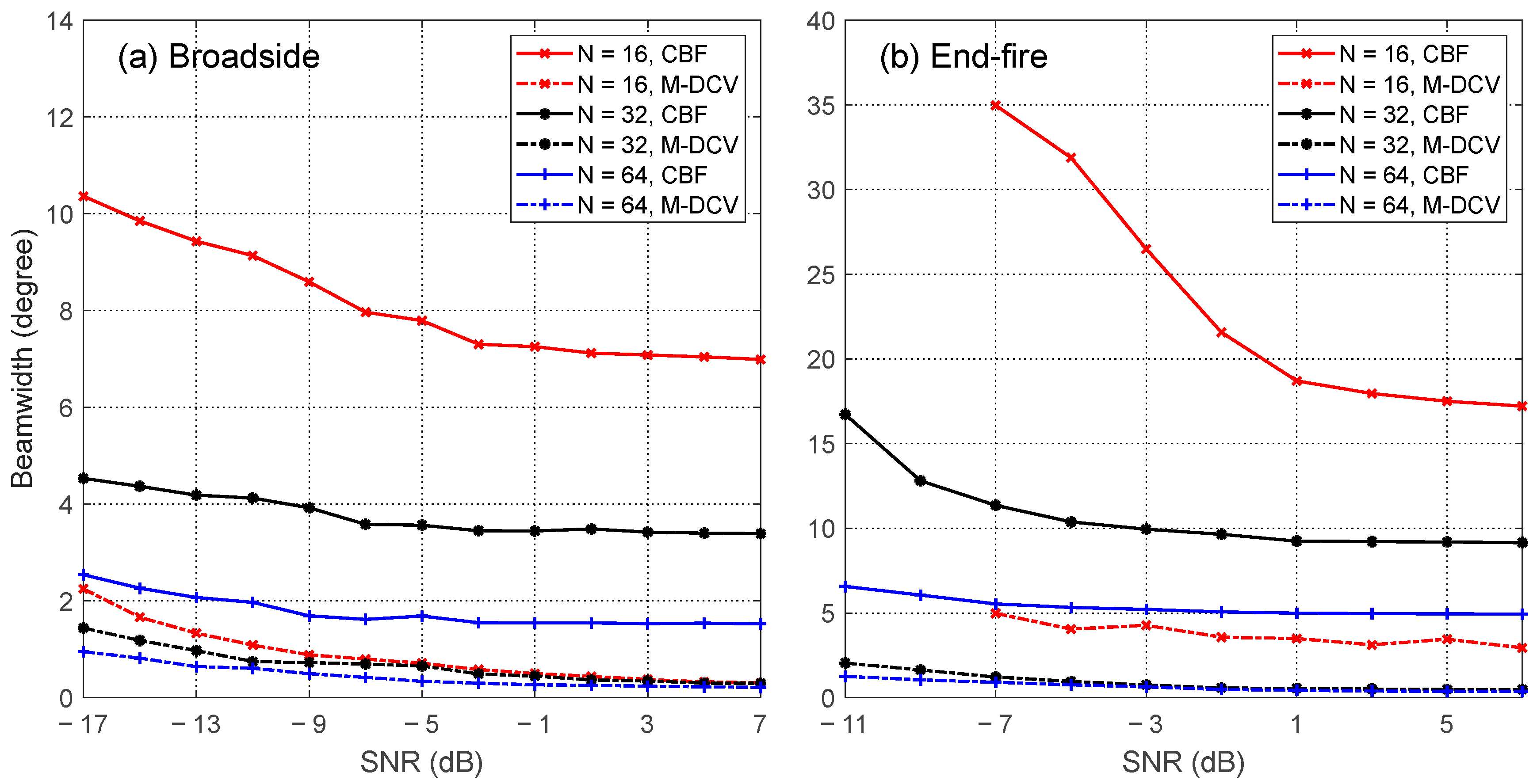
The performance of the M-DCV algorithm on angular resolution as a function of the signal-to-noise ratios (SNRs), number of array elements, and number of snapshots is then tested. The performance is evaluated according to the beam width for the M-DCV results of ideal features with negligible width located at the broadside and end-fire directions, respectively.

We first study the dependence of the beam width as a function of the SNR. The number of snapshots is constantly set to 5, and the number of array elements is fixed at 16, 32, and 64. As shown in Figure 9, the M-DCV algorithm provides an improvement of up to one order of magnitude in angular resolution compared with the CBF algorithm. For features at the array broadside (Figure 9a), the beam width of the M-DCV results gradually decreases and tends to be stable when the SNR becomes greater than −3 dB for all the arrays with different numbers of elements. For the array with 16 elements, the beam width of the M-DCV results decreases from 2.25° to 0.30°. The angular resolution is slightly improved for the array with 32 elements as the beam width decreases from 1.44° to 0.29°. The beam width can be further reduced but less improved when array elements increase to 64 as the beam width decreases from 0.95° to 0.22°. For features at the end-fire direction of the array (Figure 9b), the beam width of the M-DCV results is similar but slightly larger compared with the results at the array broadside. For the arrays with 16, 32, and 64 elements, the beam width of the M-DCV results decreases from 4.98° to 2.94°, from 2.04° to 0.48°, and from 1.26° to 0.36°, respectively. For the array with 16 elements, the initial SNR is set to −7 dB, and the beam width of the M-DCV results becomes unstable for features at the end-fire direction. This is because the array gain becomes extremely low in this condition. The steer response after beamforming is significantly affected by the noise incident from other directions, leading to an unstable feature that can hardly be determined from the beamformed intensity distribution.

We next study the dependence of the beam width as a function of the number of array elements. The number of snapshots is constantly set to 5. For features at the array broadside, the SNRs are fixed at −18 dB, −13 dB, and −8 dB, respectively. As shown in Figure 10a, the beam width of the M-DCV results decreases from 2.72° to 0.43° as the number of array elements increases from 8 to 64 for a −13 dB fixed SNR. The angular resolution is slightly improved for a higher SNR at −8 dB as the beam width decreases from 2.35° to 0.42°. The angular resolution can be further but less improved when the array elements increase to more than 64. It is noticed that, for an SNR lower than −18 dB, although the beam width maintains a downward trend, it becomes unstable since the weak fluctuating target signal is difficult to identify from the ambient noise. For features at the end-fire direction of the array, the SNRs are fixed at −8 dB, −3 dB, and 2 dB, respectively. As shown in Figure 10b, the beam width of the M-DCV results maintains a similar trend as in the broadside direction. For a fixed −8 dB SNR, the beam width decreases from 4.98° to 0.53°. For higher SNRs at −3 dB and 2 dB, the beam width of the M-DCV results decreases from 4.27° to 0.49° and from 3.54° to 0.45°, respectively. The difference in SNR settings between broadside and end-fire directions is because the array gain is lower at the end-fire direction. Any features with SNRs lower than −8 dB are hard to identify from the ambient noise.

Finally, we study the performance of the M-DCV algorithm as a function of the number of snapshots. The SNR is constantly set at −8 dB, and the number of array elements is fixed at 32. As shown in Figure 11, the performance of the M-DCV algorithm improves and stabilizes as the number of snapshots increases up to 5 for both the broadside and end-fire directions. The beam width of the M-DCV results decreases from 1.15° to 0.70° for features at the array broadside and decreases from 1.31° to 0.86° for features at the end-fire direction. For comparison, the beam width of the CBF output remains unchanged for both the broadside and end-fire directions. In most practical applications, a number of snapshots larger than 5 is required to obtain stable intensity distribution estimates via deconvolution.

3.3. Field Experiment Data Results

The field experiment was conducted near the Xisha Islands in the South China Sea in June 2021 and consisted of performing dynamic acoustic imaging of the geological features of the seabed [52] (Figure 12). The water depth in the Xisha Islands region ranges from 200 m to 1200 m. Two research vessels, Fishing & Scientific IX and Fishing & Scientific III, were employed to carry a low-frequency source array and tow a large-aperture horizontal linear hydrophone array during the experiment. The source array, consisting of ten transducer elements at a spacing of 0.417 m, was deployed vertically with a center depth of approximately 50 m from the source ship. The source ship was moored throughout the transmission, and its position information was determined and recorded using the onboard GPS sensor. The source array periodically transmitted an up-sweep linear frequency modulated (LFM) signal shaded with a Turkey window every 40 s, with a center frequency of 1800 Hz, a bandwidth of 200 Hz, and a pulse width of 1 s. The source level was calibrated as 216 dB re 1μPa @ 1m. The pulse signals propagating through the ocean acoustic waveguide were scattered by the geological features of the seabed and other potential targets. A nested array with 128 elements was towed by the receiver ship along a preset route to collect and record the echoes of the transmitted pulse signals (Figure 12). The first 96 elements of the array, with a spacing of 0.417 m, were designed for signals with a frequency below 1800 Hz, and the remaining 32 elements, with a spacing of 1.667 m, were designed for signals below 450 Hz. The sound speed was assumed to be $c=$ 1500 m/s in data processing.

The echo signal collected by the receiver array was processed to image the scattering acoustic field from the geological features of the seabed or other potential targets as a function of the incident direction and time using coherent CBF and matched filtering. We adopted the acoustic data collected by multiple sub-apertures consisting of either 16 or 32 elements with a 50% overlap throughout the array to test the performance of the M-DCV and AM-DCV algorithms. The acoustic data from all sub-apertures after CBF and normalization were averaged and used for subsequent deconvolution.

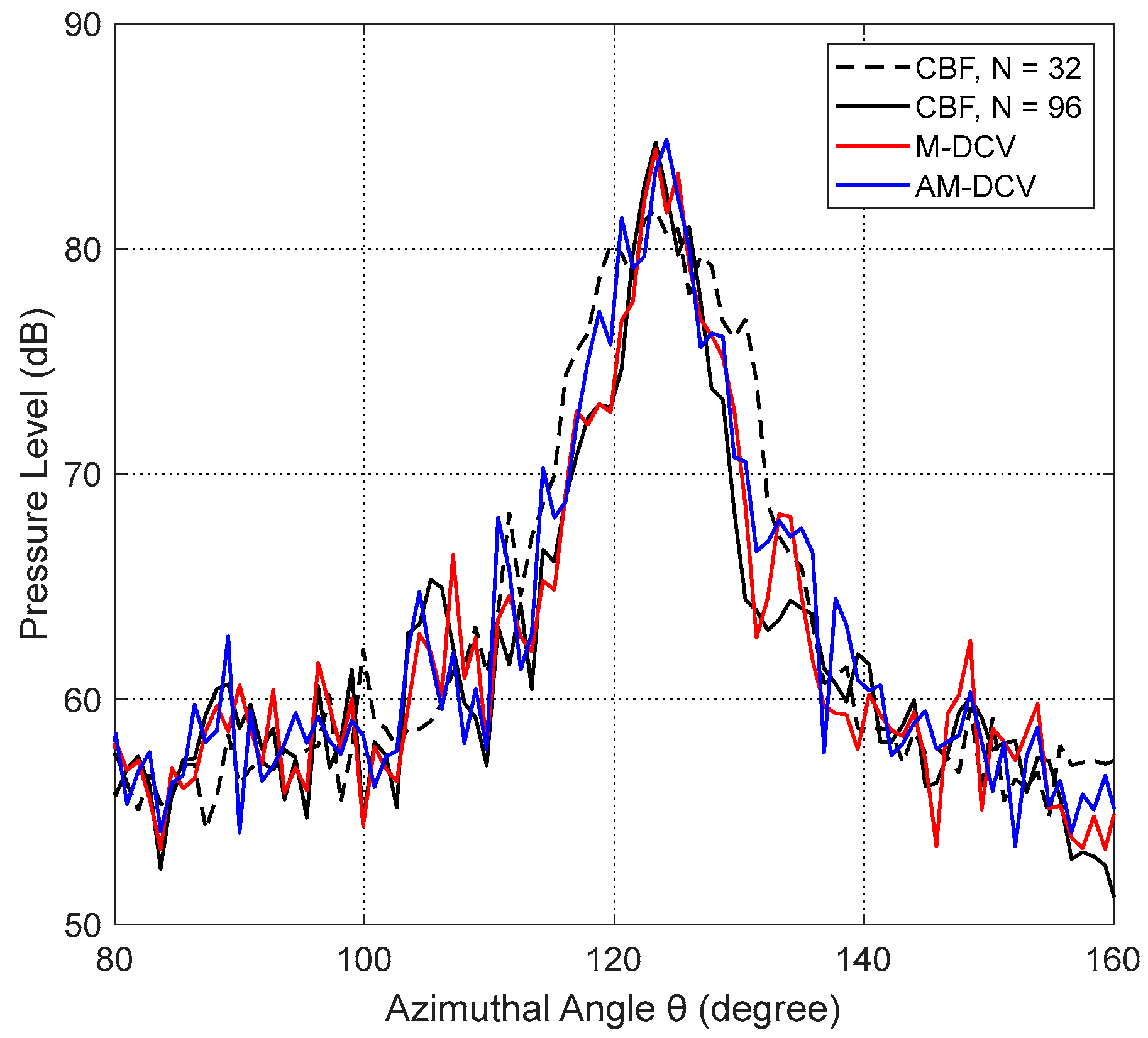
We first evaluated the performance of the M-DCV and AM-DCV algorithms for a relatively wide potential target located at the broadside direction of the receiver array. Echo signals from potential targets were recorded in the continental rise region in the area west of the Xisha Islands around 8:45 on 18 June 2021 (China Standard Time; CST). The potential target highlighted within the white box in Figure 13 is considered to be an underwater geological feature. This feature was identified by scattering echoes that were continuously received over nearly half an hour between 8:27 and 8:52 (CST); moreover, the position of the scatterer did not change over time or with the changing positions of the sound source and receiver. The M-DCV and AM-DCV algorithms were applied to the CBF outputs of echo signals using sub-apertures with 32 array elements. Figure 13 shows the results in Cartesian coordinates on the left and in polar coordinates on the right. The intensity distributions of the CBF outputs, the M-DCV and AM-DCV algorithm results averaged over a distance from 12.50 km to 12.60 km, are plotted as a function of the azimuthal angle in Figure 14. In addition, the result of the CBF outputs with a full aperture consisting of 96 array elements is shown in the figure as the ground truth for comparison. The M-DCV result of potential target imagery leads to a maximum 45% improvement in angular resolution over CBF. As shown in Figure 13, the imaging of the M-DCV and AM-DCV results, as well as the CBF outputs with the full array of 96 elements, can depict the boundary and shape of the target well, which is not achievable using the CBF with 32 elements. The M-DCV result deteriorates the ground truth intensity at up to 20 dB down from the peak value, compared with that of the CBF at roughly 4 dB from the peak value.

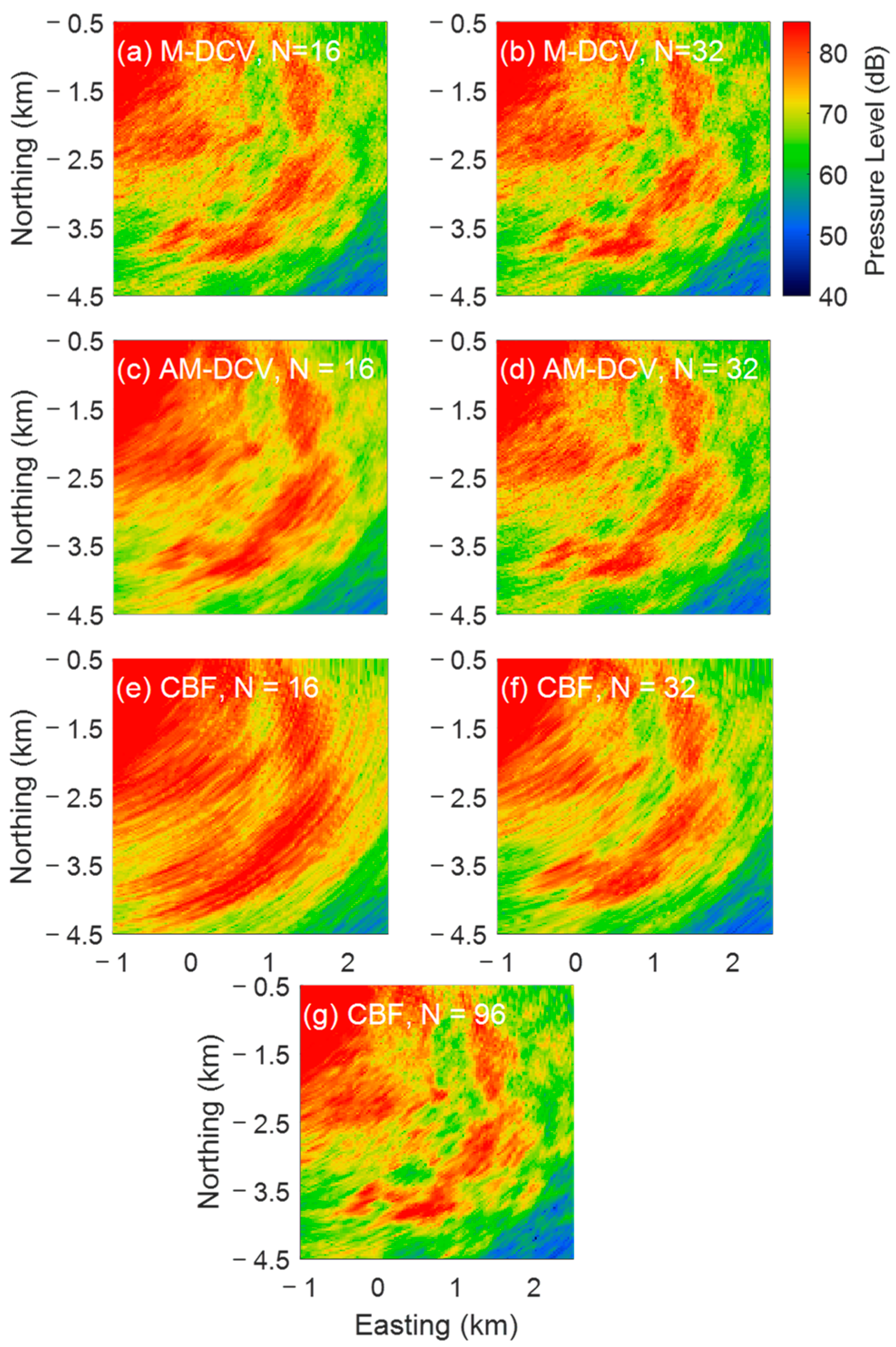
We next compare the performance of the M-DCV, AM-DCV, and CBF results for wide-range extended features detected near the South China Sea continental shelf at 20:33 on 19 June 2021 (CST). The strong scatters highlighted within the white box in Figure 15 are considered to be a result of continental shelf reverberation. Multiple eigenrays formed under the marine sound speed profile by the transmitted signals focused on the continental shelf, thereby generating reverberation echoes. The distribution of reverberation echoes is related to the seabed geographic features, water depth, sound speed profile, and the relative positions of the source and receiver. The results for sub-apertures with both 16 and 32 array elements are shown in Figure 15 to illustrate the effectiveness of the algorithm. As shown in the figure, the AM-DCV result with 32 array elements (Figure 15d) shows comparable performance to the CBF algorithm using the full aperture with 96 elements (Figure 15g). The M-DCV results with fewer than 16 array elements (Figure 15a) also achieve a similar performance (Figure 15d), indicating that the AM-DCV algorithm has a comparable performance on deconvolved beamforming as the array aperture reduction. In practical applications, the AM-DCV algorithm will greatly reduce the computation time, making it useful in applications that require quasi-instantaneous processing.

4. Discussion

In this study, we follow the well-known assumption that the instantaneous field of incident plane waves from distinct directions follows circular complex Gaussian statistics, due to random fluctuations caused by random wave propagation and scattering according to the central limit theorem [38,39,40,41]. The averaged intensity of each incident plane wave over a short time period (e.g., the measurement time) follows a Gamma distribution. As a result, the acoustic intensity measurements then derived from the CCGR field contain signal-dependent noise [37,38]. After time-harmonic plane wave beamforming with a sufficient large-aperture array, intensities at distinct scanning angles are statistically independent of each other and can be considered as a summation of the products of the beam pattern and multiple independent—but not identical—Gamma-distributed incident plane wave intensities. Knowing the beam pattern of the array with a spatial taper function, we yield a maximum likelihood estimator of the incident intensities from distinct directions through maximizing the likelihood function of these independent beams. The estimator acts as a deconvolution process that extracts the original angular distribution of the incident plane wave fields from blurred beamformed outputs.

Previous work has assumed that the beamformed intensity of incident plane waves measured at a certain scan angle follows the Gamma distribution. It is noticed that, for multiple adjacent features with significant differences in intensity, the statistics of the CBF output deviate from the Gamma distribution, leading to a noticeable performance degradation in angular resolution for the DCV algorithm. Therefore, in this study, we derive the modified conditional probability distribution of the beamformed intensity. Furthermore, we also provide an improved initial solution vector for the iterative scheme and an approximate likelihood model that can be numerically calculated.

5. Conclusions

In this study, the CBF output intensities at distinct scan angles were modeled as the summation of the products of the beam pattern and multiple independent—but not identical—Gamma-distributed incident plane wave intensities. Based on this conclusion, we derived the exact conditional probability distribution of beamformed intensity and proposed the M-DCV algorithm. We also introduced a computationally efficient approximate expression for calculating the conditional probability distribution of the CBF output. To reduce the computational complexity, we proposed the AM-DCV algorithm, which simplifies the modified model and reduces the number of random signals when calculating the conditional probability distribution. Using both synthetic and experimental data, the M-DCV and AM-DCV algorithms were shown to provide a significant improvement in angular resolution over CBF. The performance of the M-DCV algorithm was further evaluated as a function of signal-to-noise ratios, number of array elements, and number of snapshots. The M-DCV result for acoustic images generated from the real data indicated an improvement of roughly 45% close to the array broadside. The proposed algorithms are applicable for OAWRS or other applications that utilize plane wave beamforming with linear or other array types.

References

- Urick, R.J. Principles of Underwater Sound; McGraw Hill: New York, NY, USA, 1983. [Google Scholar]
- Van Trees, H.L. Detection, Estimation, and Modulation Theory, Part I; Wiley-Interscience: New York, NY, USA, 2001. [Google Scholar]
- Van Trees, H.L. Optimum Array Processing; John Wiley & Sons: Hoboken, NJ, USA, 2002. [Google Scholar]
- Makris, N.; Ratilal, P.; Jagannathan, S.; Gong, Z.; Andrews, M.; Bertsatos, I.; Godø, O.; Nero, R.; Jech, J. Critical Population Density Triggers Rapid Formation of Vast Oceanic Fish Shoals. Science 2009, 323, 1734–1737. [Google Scholar] [CrossRef]
- Makris, N.C.; Ratilal, P.; Symonds, D.T.; Jagannathan, S.; Lee, S.; Nero, R.W. Fish population and behavior revealed by instantaneous continental shelf-scale imaging. Science 2006, 311, 660–663. [Google Scholar] [CrossRef]
- Wang, D.; Garcia, H.; Huang, W.; Tran, D.D.; Jain, A.D.; Yi, D.H.; Gong, Z.; Jech, J.M.; Godø, O.R.; Makris, N.C.; et al. Vast assembly of vocal marine mammals from diverse species on fish spawning ground. Nature 2016, 531, 366–370. [Google Scholar] [CrossRef]
- Huang, W.; Wang, D.; Ratilal, P. Diel and Spatial Dependence of Humpback Song and Non-Song Vocalizations in Fish Spawning Ground. Remote Sens. 2016, 8, 712. [Google Scholar] [CrossRef]
- Makris, N. Imaging ocean-basin reverberation via inversion. J. Acoust. Soc. Am. 1993, 94, 983–993. [Google Scholar] [CrossRef]
- Swee, C.; Makris, N.; Fialkowski, L. A comparison of bistatic scattering from two geologically distinct abyssal hills. J. Acoust. Soc. Am. 2000, 108, 2053–2070. [Google Scholar] [CrossRef] [PubMed]
- Ratilal, P.; Lai, Y.; Symonds, D.; Ruhlmann, L.; Preston, J.; Scheer, E.; Garr, M.; Holland, C.; Goff, J.; Makris, N. Long range acoustic imaging of the continental shelf environment: The Acoustic Clutter Reconnaissance Experiment 2001. J. Acoust. Soc. Am. 2005, 117, 1977–1998. [Google Scholar] [CrossRef]
- Capon, J. High-Resolution Frequency-Wavenumber Spectrum Analysis. Proc. IEEE 1969, 57, 1408–1418. [Google Scholar] [CrossRef]
- Schmidt, R. Multiple Emitter Location and Signal Parameter Estimation. IEEE Trans. Antennas Propag. 1986, 34, 276–280. [Google Scholar] [CrossRef]
- Zeng, W.; So, H.C.; Huang, L. ℓp-MUSIC: Robust Direction-of-Arrival Estimator for Impulsive Noise Environments. IEEE Trans. Signal Process. 2013, 61, 4296–4308. [Google Scholar]
- He, Z.; Liu, Q.; Jin, L.; Ouyang, S. Low complexity method for DOA estimation using array covariance matrix sparse representation. Electron. Lett. 2013, 49, 228–230. [Google Scholar] [CrossRef]
- Abraham, D.; Owsley, N. Beamforming with Dominant Mode Rejection. In Proceedings of the IEEE OCEANS ′90. Engineering in the Ocean Environment, Washington, DC, USA, 24–26 September 1990; pp. 470–475. [Google Scholar]
- Ying, D.; Yan, Y. Robust and Fast Localization of Single Speech Source Using a Planar Array. IEEE Signal Process. Lett. 2013, 20, 909–913. [Google Scholar] [CrossRef]
- Malioutov, D.; Cetin, M.; Willsky, A. Sparse signal reconstruction perspective for source localization with sensor arrays. IEEE Trans. Signal Process. 2005, 53, 3010–3022. [Google Scholar] [CrossRef]
- Tropp, J.; Gilbert, A. Signal Recovery from Random Measurements via Orthogonal Matching Pursuit. IEEE Trans. Inf. Theory 2008, 53, 4655–4666. [Google Scholar] [CrossRef]
- Sahoo, S.; Makur, A. Signal Recovery from Random Measurements via Extended Orthogonal Matching Pursuit. IEEE Trans. Signal Process. 2015, 63, 2572–2581. [Google Scholar] [CrossRef]
- Chang, L.; Wu, J. An Improved RIP-Based Performance Guarantee for Sparse Signal Recovery via Orthogonal Matching Pursuit. IEEE Trans. Inf. Theory 2014, 60, 5702–5715. [Google Scholar] [CrossRef]
- Yang, Z.; Xie, L. Continuous Compressed Sensing with a Single or Multiple Measurement Vectors. In Proceedings of the 2014 IEEE Workshop on Statistical Signal Processing (SSP), Gold Coast, QLD, Australia, 29 June–2 July 2014. [Google Scholar]
- Yang, Z.; Xie, L. On gridless sparse methods for multi-snapshot DOA estimation. In Proceedings of the 2016 IEEE International Conference on Acoustics, Speech and Signal Processing (ICASSP), Shanghai, China, 20–25 March 2016. [Google Scholar]
- Yang, Z.; Xie, L. Enhancing Sparsity and Resolution via Reweighted Atomic Norm Minimization. IEEE Trans. Signal Process. 2016, 64, 995–1006. [Google Scholar] [CrossRef]
- Berger, C.; Zhou, S.; Preisig, J.; Willett, P. Sparse Channel Estimation for Multicarrier Underwater Acoustic Communication: From Subspace Methods to Compressed Sensing. IEEE Trans. Signal Process. 2010, 58, 1708–1721. [Google Scholar] [CrossRef]
- Zhang, Y.; Sun, H.; Xu, F.; Wang, D. OFDM Transform-domain Channel Estimation Based on MMSE for Underwater Acoustic Channels. In Proceedings of the 2008 2nd International Conference on Anti-Counterfeiting, Security and Identification, Guiyang, China, 20–23 August 2008; pp. 177–181. [Google Scholar]
- Liu, S.; Zuberi, H.; Lou, Y.; Farooq, B.; Shaikh, S.; Raza, W. M-ary nonlinear sine chirp spread spectrum for underwater acoustic communication based on virtual time-reversal mirror method. EURASIP J. Wirel. Commun. Netw. 2021, 2021, 112. [Google Scholar] [CrossRef]
- Berger, C.; Wang, Z.; Huang, J.; Zhou, S. Application of compressive sensing to sparse channel estimation. IEEE Commun. Mag. 2010, 48, 164–174. [Google Scholar] [CrossRef]
- Liu, Z.; Zhou, Q.; Gan, W.; Qiao, G.; Bilal, M. Adaptive Joint Channel Estimation of Digital Self-Interference Cancelation in Co-time Co-frequency Full-Duplex Underwater Acoustic Communication. In Proceedings of the 2019 IEEE International Conference on Signal, Information and Data Processing (ICSIDP), Chongqing, China, 11–13 December 2019; pp. 1–5. [Google Scholar]
- Zuberi, H.; Liu, S.; Bilal, M.; Alharbi, A.; Jaffar, A.; Mohsan, S.A.H.; Miyajan, A.; Khan, M. Deep-Neural-Network-Based Receiver Design for Downlink Non-Orthogonal Multiple-Access Underwater Acoustic Communication. J. Mar. Sci. Eng. 2023, 11, 2184. [Google Scholar] [CrossRef]
- Qiao, G.; Liu, Y.; Zhou, F.; Zhao, Y.; Mazhar, S.; Yang, G. Deep learning-based M-ary spread spectrum communication system in shallow water acoustic channel. Appl. Acoust. 2022, 192, 108742. [Google Scholar] [CrossRef]
- Zhang, Y.; Li, C.; Wang, H.; Wang, J.; Yang, F.; Meriaudeau, F. Deep learning aided OFDM receiver for underwater acoustic communications. Appl. Acoust. 2022, 187, 108515. [Google Scholar] [CrossRef]
- Yang, T. Deconvolved Conventional Beamforming for a Horizontal Line Array. IEEE J. Ocean. Eng. 2017, 43, 160–172. [Google Scholar] [CrossRef]
- Yang, T. Deconvolution of decomposed conventional beamforming. J. Acoust. Soc. Am. 2020, 148, 195–201. [Google Scholar] [CrossRef] [PubMed]
- Ratnam, M.; Anand, V.; Rosen, J. Non-linear adaptive three-dimensional imaging with interferenceless coded aperture correlation holography (I-COACH). Opt. Express 2018, 26, 18143–18154. [Google Scholar]
- Anand, V.; Han, M.; Maksimovic, J.; Ng, S.H.; Katkus, T.; Klein, A.; Bambery, K.; Tobin, M.; Vongsvivut, J.; Juodkazis, S. Single-shot mid-infrared incoherent holography using Lucy-Richardson-Rosen algorithm. Opto-Electron. Sci. 2022, 1, 210006. [Google Scholar]
- Gopinath, S.; Praveen, P.A.; Kahro, T.; Bleahu, A.-I.; Arockiaraj, F.; Smith, D.; Ng, S.H.; Tamm, A.; Kukli, K.; Juodkazis, S.; et al. Implementation of a Large-Area Diffractive Lens Using Multiple Sub-Aperture Diffractive Lenses and Computational Reconstruction. Photonics 2022, 10, 3. [Google Scholar] [CrossRef]
- Jain, A.; Makris, N. Maximum Likelihood Deconvolution of Beamformed Images with Signal-Dependent Speckle Fluctuations from Gaussian Random Fields: With Application to Ocean Acoustic Waveguide Remote Sensing (OAWRS). Remote Sens. 2016, 8, 694. [Google Scholar] [CrossRef]
- Makris, N. The effect of saturated transmission scintillation on ocean acoustic intensity measurements. J. Acoust. Soc. Am. 1996, 100, 769–783. [Google Scholar] [CrossRef]
- Makris, N. Parameter resolution bounds that depend on sample size. J. Acoust. Soc. Am. 1996, 99, 2851–2861. [Google Scholar] [CrossRef]
- Jagannathan, S.; Küsel, E.; Ratilal, P.; Makris, N. Scattering from extended targets in range-dependent fluctuating ocean-waveguides with clutter from theory and experiments. J. Acoust. Soc. Am. 2012, 132, 680–693. [Google Scholar] [CrossRef] [PubMed]
- Tran, D.; Ratilal, P. Probability distribution for energy of saturated broadband ocean acoustic transmission: Results from Gulf of Maine 2006 experiment. J. Acoust. Soc. Am. 2013, 133, 3346. [Google Scholar] [CrossRef]
- Goodman, J.W. Statistical Optics; Wiley-Interscience: New York, NY, USA, 1985. [Google Scholar]
- Kelley, C. Iterative Methods for Optimization; Society for Industrial & Applied Mathematics (SIAM): Philadelphia, PA, USA, 1999; Volume 18. [Google Scholar]
- Wang, D.; Ratilal, P. Angular Resolution Enhancement Provided by Nonuniformly-Spaced Linear Hydrophone Arrays in Ocean Acoustic Waveguide Remote Sensing. Remote Sens. 2017, 9, 1036. [Google Scholar] [CrossRef]
- Makris, N. A foundation for logarithmic measures of fluctuating intensity in pattern recognition. Opt. Lett. 1995, 20, 2012–2014. [Google Scholar] [CrossRef] [PubMed]
- Diaconis, P.; Perlman, M. Bounds for tail probabilities of weighted sums of independent gamma random variables. Lect. Notes-Monogr. Ser. 1990, 16, 147–166. [Google Scholar]
- Mathai, A. Storage capacity of a dam with gamma type inputs. Ann. Inst. Stat. Math. 1982, 34, 591–597. [Google Scholar] [CrossRef]
- Moschopoulos, P. The Distribution of the Sum of Independent Gamma Random Variables. Ann. Inst. Stat. Math. 1985, 37, 541–544. [Google Scholar] [CrossRef]
- Akkouchi, M. On the convolution of gamma distributions. Soochow J. Math. 2005, 31, 205–211. [Google Scholar]
- Murakami, H. Approximations to the distribution of sum of independent non-identically gamma random variables. Math. Sci. 2015, 9, 205–213. [Google Scholar] [CrossRef]
- Barnabani, M. An approximation to the convolution of Gamma Distributions. Commun. Stat. Simul. Comput. 2015, 46, 331–343. [Google Scholar] [CrossRef]
- Liang, J.; Zhang, T.; Xu, W.; Zhao, H. A Linear Near-Field Interference Cancellation Method Based on Deconvolved Conventional Beamformer Using Fresnel Approximation. IEEE J. Ocean. Eng. A J. Devoted Appl. Electr. Electron. Eng. Ocean. Environ. 2023, 48, 365–371. [Google Scholar] [CrossRef]
Figure 1.
A sketch of the array geometry and incident plane wave field. The uniformly spaced linear array is aligned horizontally along the -axis in the ocean, with elements located at . The azimuthal angle of the incident plane wave is measured from the array broadside.
Figure 2.
Statistical histograms of normalized beamforming outputs at different scan angles. The conditional probability distributions are plotted with black lines.
Figure 3.
The shape parameter of the Gamma-distributed beamformed intensity of ambient noise as a function of scan angle .
Figure 4.
The results for a narrow feature of 2° width at the array broadside: (a) ground truth expected plane wave intensity and plane wave intensity with signal-dependent noise; (b) a comparison between the CBF, M-DCV, AM-DCV, DCV, and RL results; (c) a zoomed-in version of (b) within the highlighted box. The horizontal bars in (c) represent the 3 dB widths.
Figure 5.
The results for a wide feature of 9° width at the array broadside: (a) ground truth expected plane wave intensity and plane wave intensity with signal-dependent noise; (b) a comparison between the CBF, M-DCV, AM-DCV, DCV, and RL results; (c) a zoomed-in version of (b) within the highlighted box. The horizontal bars in (c) represent the 3 dB widths.
Figure 6.
The results for a narrow feature of 2° width close to the end-fire direction of the array: (a) ground truth expected plane wave intensity and plane wave intensity with signal-dependent noise; (b) a comparison between the CBF, M-DCV, AM-DCV, DCV, and RL results; (c) a zoomed-in version of (b) within the highlighted box. The horizontal bars in (c) represent the 3 dB widths.
Figure 7.
The results for a wide feature of 9° width close to the end-fire direction of the array: (a) ground truth expected plane wave intensity and plane wave intensity with signal-dependent noise; (b) a comparison between the CBF, M-DCV, AM-DCV, DCV, and RL results; (c) a zoomed-in version of (b) within the highlighted box. The horizontal bars in (c) represent the 3 dB widths.
Figure 8.
The results for two adjacent features with a relatively narrow width of 1°, a separation of 2°, and a target strength difference of 7 dB at the array broadside: (a) ground truth expected plane wave intensity and plane wave intensity with signal-dependent noise; (b) a comparison between the CBF, M-DCV, AM-DCV, DCV, and RL results; (c) a zoomed-in version of (b) within the highlighted box. The horizontal bars in (c) represent the 3 dB widths.
Figure 9.
The performance of the M-DCV algorithm as a function of signal-to-noise ratios (SNRs). The performance is evaluated according to the beam width of the CBF outputs and the M-DCV results located at (a) the broadside and (b) end-fire directions, respectively.
Figure 10.
The performance of the M-DCV algorithm as a function of the number of array elements. The performance is evaluated according to the beam width of the CBF outputs and the M-DCV results located at (a) broadside and (b) end-fire directions, respectively.
Figure 11.
The performance of the M-DCV algorithm as a function of the number of snapshots. The performance is evaluated according to the beam width of the CBF outputs and the M-DCV results located at (a) broadside and (b) end-fire directions, respectively.
Figure 12.
(a) Areal bathymetry of the location of the two ocean acoustical experiments: (b) contour map of the continental rise region in the area west of the Xisha Islands; (c) contour map of the southern flank of the continental shelf in the region south of Hainan Island, China.
Figure 13.
A comparison between (a,b) the M-DCV results using 32 array elements, (c,d) the AM-DCV results using 32 array elements, (e,f) the normalized CBF results using 32 array elements, and (g,h) the normalized CBF results using 96 array elements for a relatively wide feature in the array broadside. The subgraphs (a,c,e,g) are plotted in the Cartesian coordinate and the subgraphs (b,d,f,h) are plotted in the polar coordinate.
Figure 14.
A comparison between the intensity distributions of the normalized CBF, M-DCV, and AM-DCV results for the feature in Figure 13.
Figure 15.
A comparison between (a,b) the M-DCV results using 16 or 32 array elements, (c,d) the AM-DCV results using 16 or 32 array elements, and (e,f,g) the normalized CBF results using 16, 32 or 96 array elements for wide-range extended features detected near the South China Sea continental shelf.