Article

Evaluation of Sub-Pixel Cloud Noises on MODIS Daily Spectral Indices Based on in situ Measurements

1
Earth Observation Research Center (EORC), Japan Aerospace Exploration Agency (JAXA), 2-1-1 Sengen, Tsukuba, Ibaraki 305-8505, Japan
2
Graduate School of Life and Environment Sciences, University of Tsukuba, 1-1-1 Tennoudai, Tsukuba, Ibaraki 305-8572, Japan
3
Research Institute for Global Change, Japan Agency for Marine-Earth Science and Technology (JAMSTEC), 3173-25 Showa-machi, Kanazawa-ku, Yokohama 236-0001, Japan
*
Author to whom correspondence should be addressed.
Remote Sens. 2011, 3(8), 1644-1662; https://doi.org/10.3390/rs3081644
Submission received: 8 June 2011 / Revised: 12 July 2011 / Accepted: 27 July 2011 / Published: 3 August 2011

Abstract

:
Cloud contamination is one of the severest problems for the time-series analysis of optical remote sensing data such as vegetation phenology detection. Sub-pixel clouds are especially difficult to identify and remove. It is important for accuracy improvement in various terrestrial remote sensing applications to clarify the influence of these residual clouds on spectral vegetation indices. This study investigated the noises caused by residual sub-pixel clouds on several frequently-used spectral indices (NDVI, EVI, EVI2, NDWI, and NDII) by using in situ spectral data and sky photographs at the satellite overpass time. We conducted in situ continuous observation at a Japanese deciduous forest for over a year and compared the MODIS spectral indices with the cloud-free in situ spectral indices. Our results revealed that residual sub-pixel clouds potentially contaminated about 40% of the MODIS data after cloud screening by the state flag of MOD09 product. These residual clouds significantly decreased NDVI values during the leaf growing season. However, such noises did not appear in the other indices. This result was thought to be caused by the different combination of wavelengths among spectral indices. Our results suggested that the noises by residual sub-pixel clouds can be reduced by using EVI, NDWI, or NDII in place of NDVI.

1. Introduction

Remotely sensed spectral indices calculated from a combination of band reflectances are widely used to monitor biophysical quantities related to the terrestrial ecosystem, such as leaf area index [1,2,3,4] and leaf onset/offset phenology [5,6]. However, occasionally, clouds contaminate these data, and therefore, obscure the monitoring by optical remote sensing satellites. In particular, clouds smaller than a satellite image pixel, i.e., sub-pixel clouds, often hinder the retrieval of biophysical parameters of the ecosystem from spectral indices. Although cloud masks have been produced and demonstrated to be effective [7], they are not always able to completely offset the contamination caused by clouds [8]. Noise due to irremovable clouds is one of the severest problems for time-series monitoring using satellite sensors with low-to-medium spatial resolution (i.e., 250–1,000 m) such as the Terra/Aqua moderate resolution imaging spectroradiometer (MODIS).
To completely remove cloud noise from time-series spectral indices data, we should first understand the behavior of cloud noise in several frequently used spectral indices. Normalized difference vegetation index (NDVI) [9] is the most widely used spectral index for monitoring vegetation changes. Clouds generally show high reflectance in the visible and near-infrared domains (300–1,000 nm), which results in lower NDVI values in comparison to vegetation [10]. Based on this knowledge, several cloud-screening techniques for time-series NDVI have been developed [11,12,13]. The numerical simulation for the effect of sub-pixel clouds showed that it also led to a measurable decrease of NDVI [14]. However, the actual impact of sub-pixel clouds is not entirely clear since it is difficult to quantify clouds at the sub-pixel scale. Furthermore, for other frequently used spectral indices such as the enhanced vegetation index (EVI) [15], 2-band EVI (EVI2) [16], normalized difference water index (NDWI) [17], and normalized difference infrared index (NDII) [18,19], the effects of cloud contamination are not well understood. We hypothesize that different spectral indices may also show different responses to cloud contamination because the reflectance of different wavelength domains may show different responses to cloud contamination.
In this study, we investigated the effects of cloud contamination on several widely used spectral indices measured by the MODIS sensor: NDVI, EVI, EVI2, NDWI, and NDII. To evaluate the sub‑pixel cloud noise in satellite data, we conducted highly-frequent automatic in situ measurements using spectral radiometers and digital cameras. These measurements provided a set of hyper-spectral reflectances of the ground surface and hemispherical photos of the cloud conditions in the sky at the satellite overpass time. Several papers have demonstrated the usefulness of these monitoring systems when evaluating ecological remote sensing [20,21,22,23]. We evaluated the residual sub-pixel cloud noise by comparing the MODIS data with the in situ data.

2. Materials and Methods
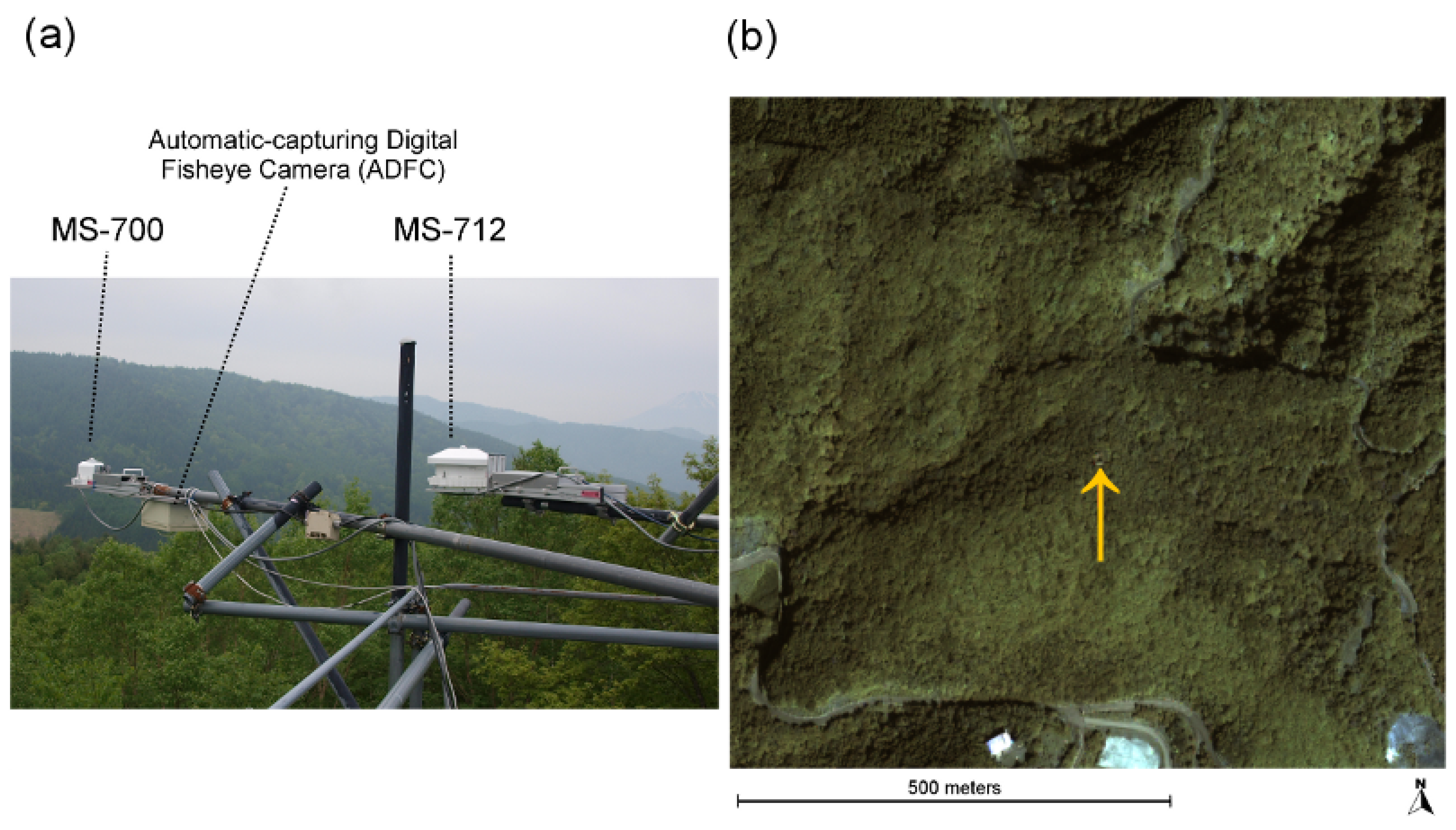
2.1. Study Site

The study site is a cool-temperate deciduous broadleaved forest near Takayama City in central Japan (137.4231°E, 36.1462°N, 1,420 m a.s.l. (above sea level) in WGS84). The annual mean air temperature and annual precipitation from 1980 to 2002 were 7.2 °C and 2,275 mm, respectively. The site is covered with snow from around December to April. Tree census and flux measurements were carried out over a 10-year period [24,25,26,27,28]. The forest canopy is dominated by Erman’s birch (Betula ermanii)and Japanese oak (Quercus crispula) [29]. The height of the dominant canopy trees ranges from 13 to 20 m. The forest floor is covered with evergreen dwarf bamboo (Sasa senanensis) with a height of 1.0 to 1.5 m. This site belongs to several monitoring networks: the Phenological Eyes Network [30] (http://www.pheno-eye.org/), JapanFlux network (http://www.japanflux.org/), and JaLTER (Japan Long-Term Research Network; http://www.jalter.org/).

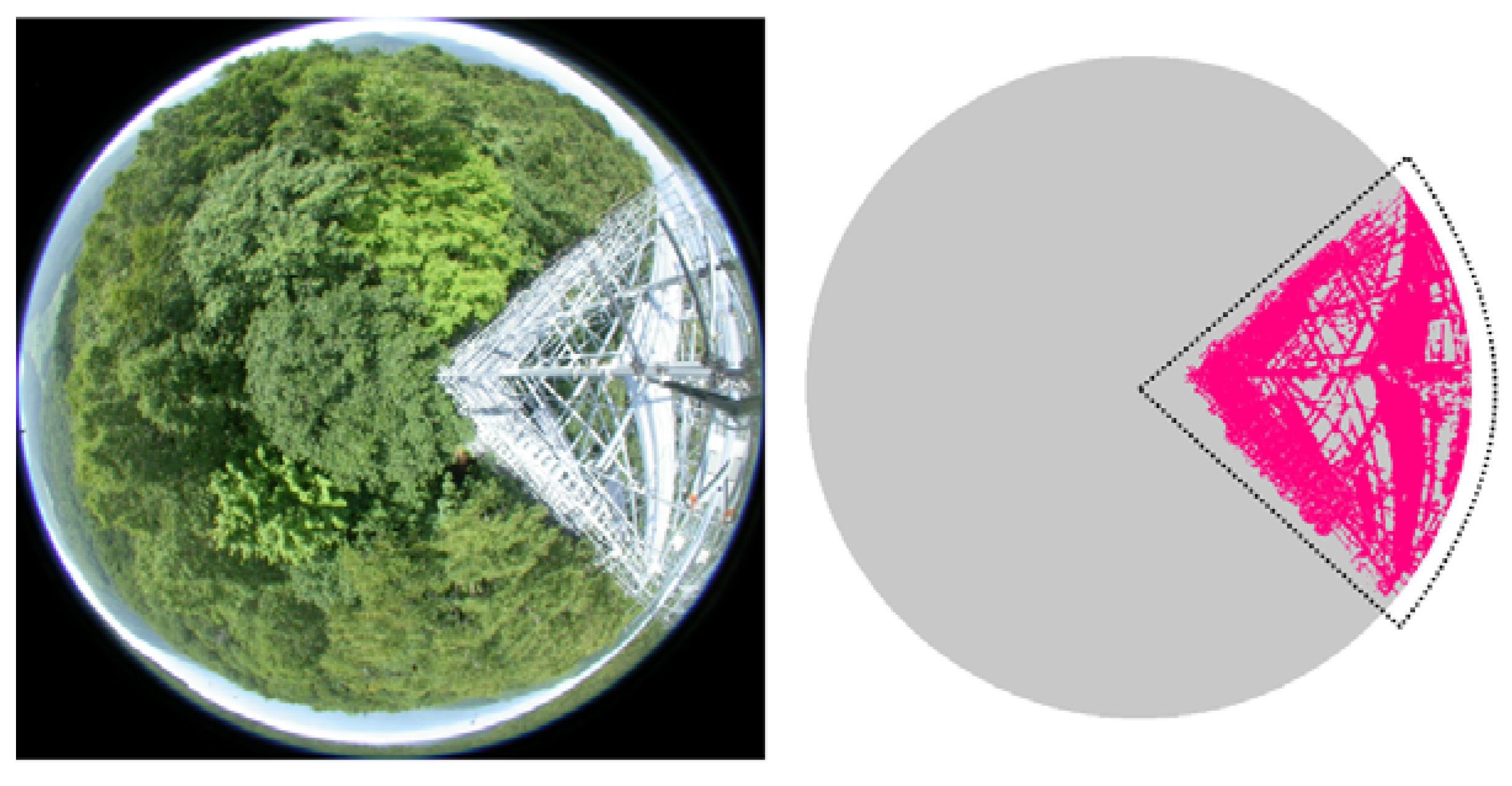
2.2. In situ Measurements

We periodically and automatically observed spectral irradiance of the sky and forest canopy by using two hemispherical spectroradiometers (HSSRs) MS-700 and MS-712 (EKO Instrument Co. Ltd., Tokyo, Japan) (Table 1). We used the automatic rotating stage CHS-AR (Hayasaka Rikoh Co. Ltd., Sapporo, Japan), which can flip back and forth and is driven by an electric motor, to enable an HSSR to observe both the downward and upward directions in alternating fashion. The HSSRs and rotating stages were installed atop an 18-m canopy-access tower facing southeast (Figure 1(a)), and they were controlled by a personal computer and manufacturer-supplied software. We setup the HSSRs to observe both the downward and the upward directions at 10-min intervals from 10:00 to 14:00 Japan Standard Time (JST) every day. Data obtained from DOY120, 2008 (29 April) until DOY365, 2009 (31 December) were used for analysis. Instrument failure resulted in more than seven days of missing data during the following periods: DOY150–158, 2008; DOY49–58, 2009; DOY62–82, 2009; DOY182–258, 2009; DOY297–316, 2009; DOY331–341, 2009.
Table 1. Specifications of the MS-700 and MS-712 spectroradiometers.
SpecificationsMS-700MS-712
Wavelength range (nm)350–1,050900–1,700
Wavelength interval (nm)3.31.56
Number of bands256512
Spectral resolution (half-bandwidth; nm)107
Wavelength accuracy (nm)±0.3±0.2
Aperture angle (°)180180
Figure 1. (a) Photo of the in situ observation system taken on 7 June 2010. (b) Pan-sharpened image by Quickbird on 3 October 2002 (image source and copyright: Digital Globe, CO, USA). The spatial resolution of the image is 0.6 m. The yellow arrow in the image indicates the location of the canopy-access tower.
Remotesensing 03 01644 g001
We also monitored the sky and forest canopy conditions by using automatic-capturing digital fisheye cameras (ADFC) (CoolPix-4500 digital camera, Nikon Corporation, Tokyo, Japan) with a fish-eye lens FC-E8 (Nikon Corporation, Tokyo, Japan; Equisolid Angle Projection) stored in a custom-built housing SPC31A (Hayasaka Rikoh Co., Ltd., Sapporo, Japan). We installed the ADFCs for the downward and the upward directions atop the 18-m canopy-access tower. The downward ADFC was installed next to the HSSRs to monitor their field of view. To control the camera functions (e.g., parameter configuration, image capture, and data retrieval), we used the free software “photopc” (http://photopc.sourceforge.net/) on the personal computers. The configuration of the cameras was as follows: mode, programmed auto; white balance, sunny or auto; fisheye mode, fisheye-1 (circular); image size, 2,272 × 1,704 pixels; and file format, JPEG. We set the cameras to capture the sky and the forest canopy at 2-min and 90-min intervals, respectively.
The area for a 250 m radius around the canopy-access tower was almost covered with deciduous forest according to the high-resolution satellite image shown in Figure 1(b). Ohtsuka et al. [24] reported that the basal area of deciduous broadleaved trees accounted for approximately 95% of the total basal area in a 100 m × 100 m plot adjacent to the northwest of the canopy-access tower. The field view of the HSSRs, which was largely consistent with the area shown in the ADFC photos (the area about a 10 m radius in following figure), also consisted of the same deciduous broadleaved trees.

2.3. Calculation of Spectral Reflectance from in situ Data

To correct the instrumental error between the MS-700 and MS-712, the spectral irradiance by MS-712 was adjusted to the spectral irradiance by MS-700 by comparing the data for the 900–1,000 nm wavelength domain (i.e., empirical linear regression). We then converted the spectral irradiance into band-averaged irradiance by using the following weighted function [31]:
I b a n d = i = λ 1 λ 2 w i I i i = λ 1 λ 2 w i
where Ii is the spectral irradiance at each wavelength, Iband is the band-averaged irradiance, and wi is the relative spectral response (RSR) of Terra MODIS bands 1–6 (Figure 2) as a function of wavelength λ. We did not use the RSR of Aqua MODIS because the RSRs of Terra MODIS and Aqua MODIS were not very different, as shown in Figure 2. The irradiances of bands 1, 2, 3, and 4 were obtained from the MS-700 data and the irradiances of bands 5 and 6 were obtained from the MS-712 data. We obtained the daily band-averaged irradiance by averaging the band-averaged irradiance measured from 10:00 to 14:00 each day because this time slot was less affected by low sun elevation angles and a shadow of the canopy-access tower. We then calculated the daily band-averaged reflectance by dividing the daily band-averaged irradiance of the ground by that of the sky. By referring to the ADFC images, data taken under rainy conditions were discarded and only data collected under sunny or cloudy conditions were used for analysis.
Figure 2. Spectral reflectance measured by the spectroradiometers (MS-700 and MS-712) on DOY 278, 2008 and relative spectral response (RSR) of Terra/Aqua MODIS bands 1–6.
Remotesensing 03 01644 g002
Because the canopy-access tower also comes into the field of view (FOV) of the HSSRs, we corrected the contamination of the tower reflectance. Using the linear mixture model theory [32], we assumed that the reflectance measured by the HSSRs (ρHSSR) can be expressed by the following equation:
ρ HSSR = f t ρ tower + ( 1 f t ) ρ canopy
where ft is the coverage of the tower to the FOV of the HSSRs, ρtower is the reflectance of the tower, and ρcanopy is the reflectance of the forest canopy. For simplicity, we did not consider the directional variation of the reflectance (i.e., bi-directional reflectance function) from the canopy and tower. We obtained ρcanopy by substituting the values of ρHSSR, ρtower, and ft into the above equation. For ρHSSR, we used the daily band-averaged reflectances measured by the HSSRs. For ρtower, we used the reflectance of the tower’s iron pipe measured by the Fieldspec FR spectroradiometer (ASD Inc., Boulder, CO, USA; Figure 3). For ft, we used ft = 0.11, which was determined by the following ADFC image analysis. We first extracted the pixels of the canopy-access tower to meet both of the following criteria determined through trial and error:
DNblue < DNgreen
DNblue > 200
where DNblue and DNgreen are the 1-byte digital numbers (0–255) of blue and green, respectively. We then calculated the ratio of the number of extracted pixels to the number of total pixels, which was regarded as the coverage of the canopy-access tower (Figure 4).
Figure 3. Spectral reflectance of the tower’s iron pipe as measured by the Fieldspec (FR) spectroradiometer on DOY 301, 2004, and the corrected and non-corrected spectral reflectances measured by MS-700 and MS-712 on DOY 278, 2008.
Remotesensing 03 01644 g003
Figure 4. Automatic-capturing digital fisheye camera (ADFC) image used for extracting the area of canopy-access tower. This image was taken on DOY 220, 2008. The red pixels in the right image were extracted as the canopy-access tower. We applied the extraction of the tower pixels for the region enclosed by the dotted line in the right image.
Remotesensing 03 01644 g004

2.4. Processing of Terra/Aqua MODIS Data

We used the data from the MODIS sensor onboard the Terra and Aqua satellites. We downloaded the products of atmospherically corrected surface reflectance data (MOD09GA and MYD09GA; daily temporal resolution; 500-m and 1-km spatial resolution; collection 5) from the NASA Land Processes Distributed Active Archive Center (LP DAAC, https://lpdaac.usgs.gov/). The MOD09GA product was obtained by the Terra MODIS in the morning during its descending orbit, and the MYD09GA product was obtained by the Aqua MODIS in the afternoon during its ascending orbit. In the 36 spectral bands of MODIS, we used the data of bands 1–3, 5, and 6 with 500-m spatial resolution. The conversion of map projections was performed by using the MODIS Reprojection Tool provided by the LP DAAC. The integrated sinusoidal (ISIN) projection of the original data was converted into a geographic projection (datum, WGS84; sampling protocol, nearest neighbor; output pixel size, 0.004167°). We then extracted the values of the band reflectance, quality control (QC) flag, state flag (including a cloud mask), and sensor zenith angle of the pixel over the study site. By referring to the QC flag, data with sensor troubles were discarded. To evaluate cloud noise that could not be removed by the cloud mask, only data with a ‘clear’ cloud state flag were used; data with ‘cloudy’, ‘mixed’, and ‘not set’ flags were not used. We also only used the data taken when the sensor zenith angle was less than 50° to avoid degradation of the spatial resolution due to large sensor zenith angles.

2.5. Calculation of Spectral Indices

We calculated NDVI [9], EVI [15], EVI2 [16], NDWI [17], and NDII [18,19] from the in situ band-reflectance and MODIS band-reflectance by using the following equations:
N D V I = B 2 B 1 B 2 + B 1
E V I = G B 2 B 1 B 2 + C 1 B 1 C 2 B 3 + L
E V I 2 = G B 2 B 1 B 2 + ( 6 7.5 / c ) B 1 + 1
N D W I = B 2 B 5 B 2 + B 6
N D I I = B 2 B 6 B 2 + B 6
where B1, B2, B3, B5, and B6 are the reflectances of MODIS bands 1, 2, 3, 5, and 6, respectively (Figure 2). In the calculation of EVI, we adopted L = 1, C1 = 6, C2 = 7.5, and G = 2.5 in reference to Huete et al. [15]. For EVI2, we adopted c = 2.08 and G = 2.5 in reference to Jiang et al. [16]. EVI was designed to reduce the influences of saturation for high-biomass vegetation, canopy-background reflectance, and residues of atmospheric correction in the NDVI value [15]. EVI2 was developed to show a change similar to the original 3-band EVI without using a blue band [16]. NDWI and NDII are often used for monitoring the water cover or content of the ground surface [33,34,35].

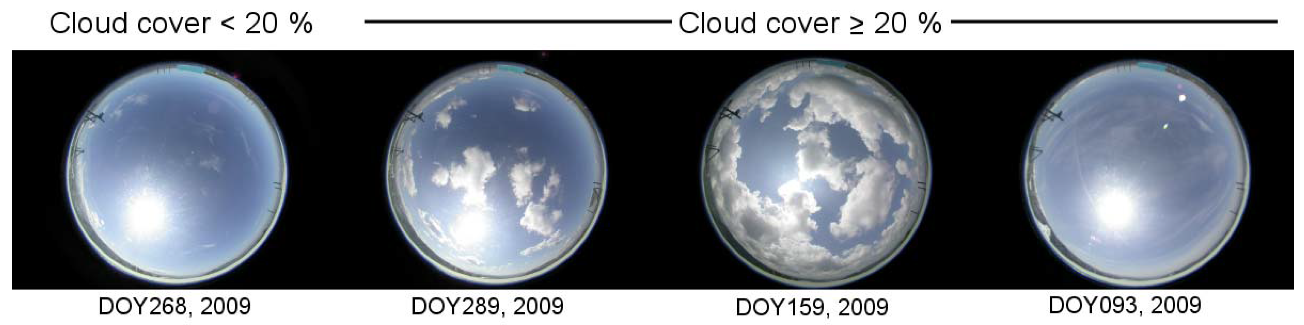
2.6. Cloud Coverage at the MODIS Overpass Time

We assessed sky conditions at the overpass times of Terra/Aqua MODIS using the ADFC images. The Terra/Aqua overpass time each day was obtained from the L1A geolocation fields product (MOD03/MYD03, 1-km resolution, collection 5). The MOD03/MYD03 products were downloaded from the Level 1 and Atmospheric Archive and Distribution System (LAADS, http://ladsweb.nascom.nasa.gov). The original map projection was converted into a geographic projection (datum, WGS84; sampling protocol, nearest neighbor; output pixel size, 0.008333°) using the MODIS Swath Reprojection Tool provided by the LP DAAC.
We only used the data with a ‘clear’ cloud state flag for the MOD09/MYD09 products, but several data were still measured under cloudy conditions according to the ADFC sky images. Therefore, we classified the data into three categories in terms of the cloud coverage in the ADFC image at the overpass time as interpreted by the human eye (Figure 5):
  • Category 1: cloud coverage of the sky was less than 20%;
  • Category 2: cloud coverage was more than 20%;
  • Category 3: cloud coverage was unknown because of missing ADFC images.
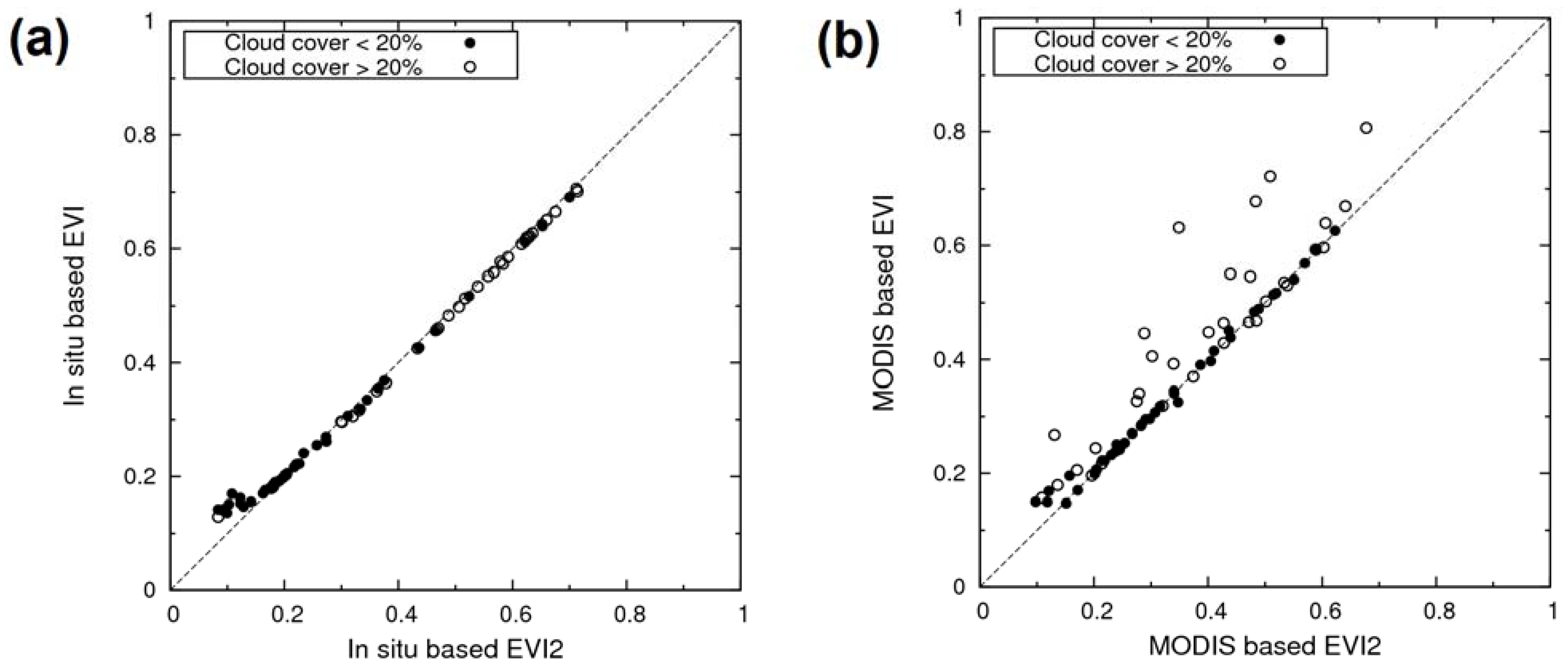
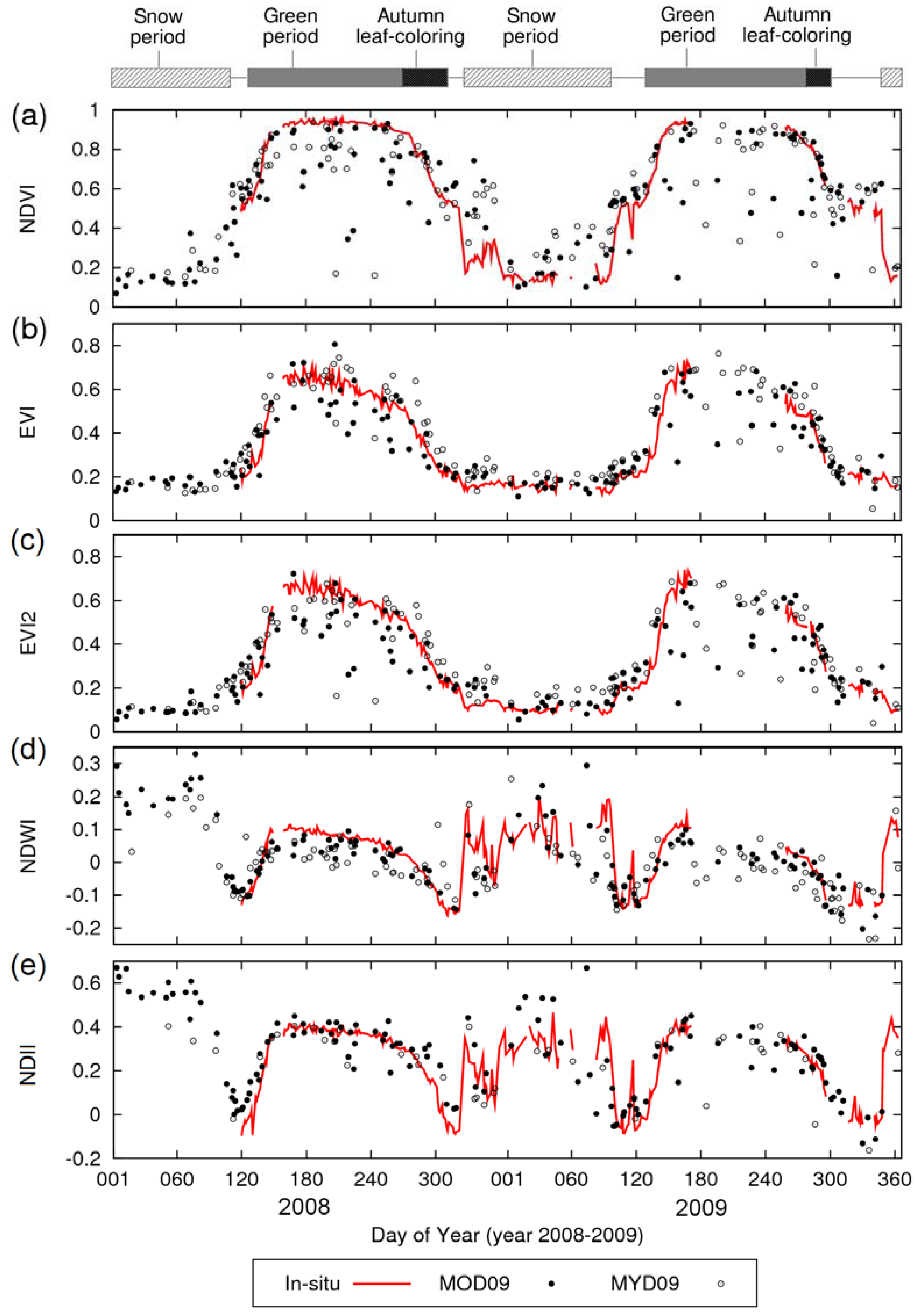
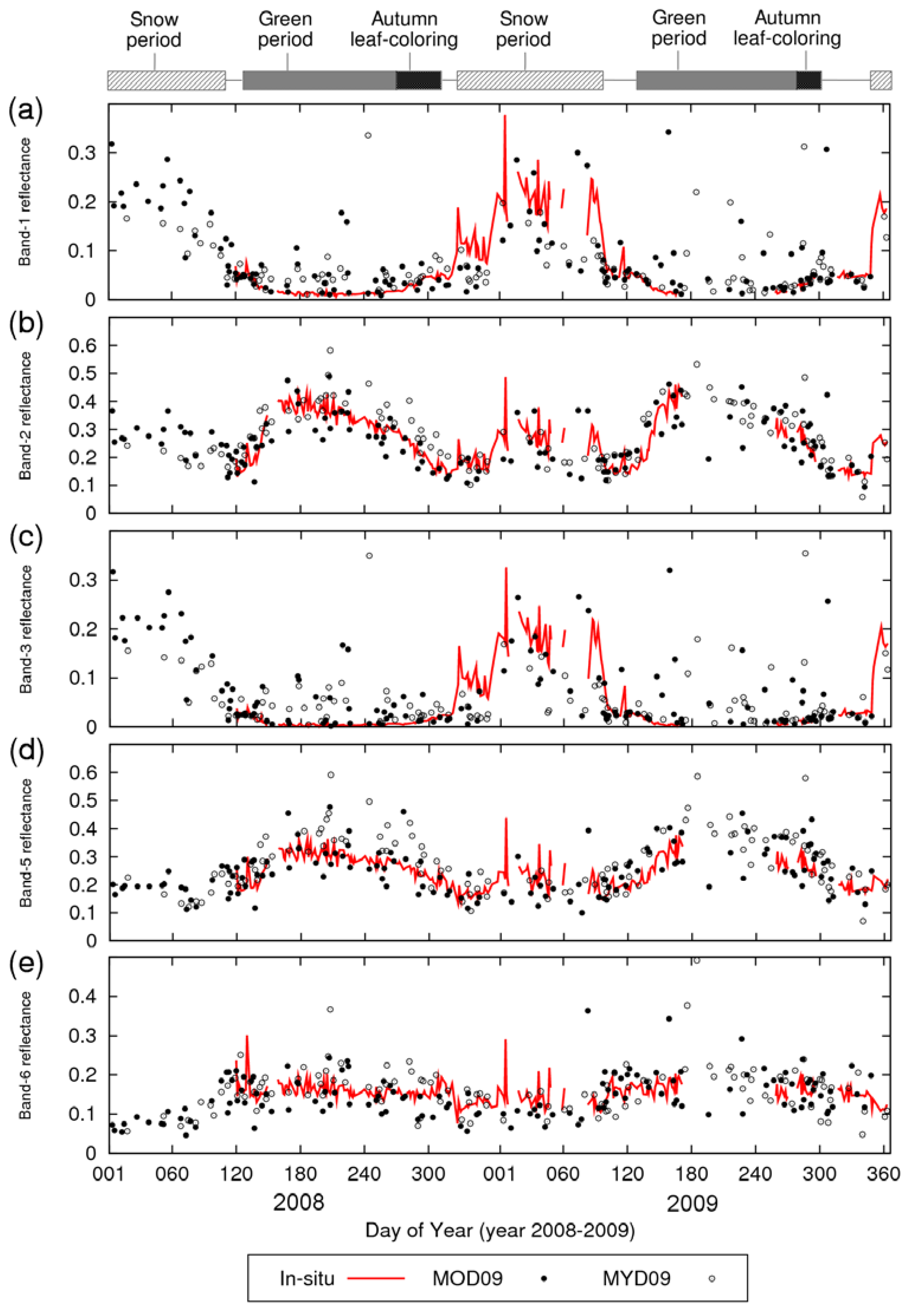
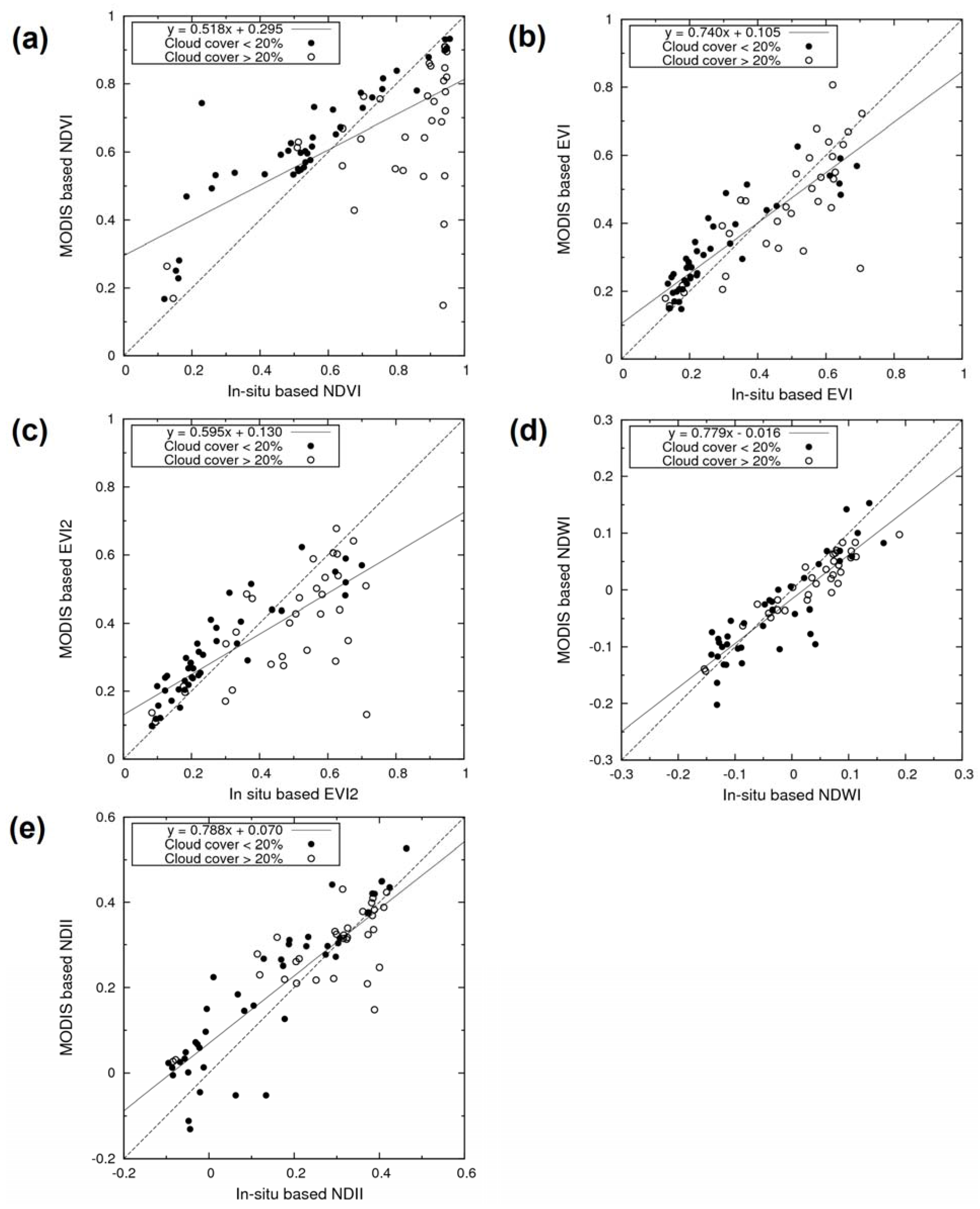
We included thin clouds over the sky in category 2 because the coverage was difficult to estimate with the human eye.
Figure 5. Examples of cloud classification for ADFC sky images at the MODIS overpass time.
Remotesensing 03 01644 g005

3. Results

Seasonal changes in the MODIS spectral indices were roughly in accordance with the in situ spectral indices (Figure 6). All of the in situ spectral indices rapidly increased during the leaf green-up period in spring (DOY 130–150) and decreased during the leaf senescence period in autumn (DOY 270–300). When the ground was covered with snow, NDVI, EVI, and EVI2 showed their minimum values for the year (about 0.1 for NDVI and EVI); on the other hand, NDWI and NDII showed maximum values for the year (about 0.3 for NDWI, 0.6 for NDII). These characteristics were also found in the spectral indices observed by the MODIS sensors, but the MODIS spectral indices were sometimes systematically higher than the in situ spectral indices at the start and end of the growing period.
Figure 6. Seasonal changes in spectral indices as measured by the ground spectroradiometers (HSSRs) and Terra/Aqua MODIS: (a) NDVI, (b) EVI, (c) EVI2, (d) NDWI, and (e) NDII. The top horizontal box diagram represents the condition of the site observed from the canopy photos. We discarded the data with sensor trouble or cloud contamination with reference to the QC flag and state flag; we also discarded data captured when the sensor zenith angle was more than 50°.
Remotesensing 03 01644 g006
Figure 7 shows the seasonal changes in the band reflectances observed by MODIS and in situ HSSRs. For both the MODIS data and the in situ data, the reflectance of bands 1 and 3 became relatively low during the growing period; on the other hand, the reflectance of bands 2, 5, and 6 became relatively high during the growing period. The MODIS measured reflectances showed some fluctuations around the in situ reflectances.
Figure 7. Seasonal changes in MODIS band reflectances measured by the ground spectroradiometers (HSSRs) and Terra/Aqua MODIS: (a) band 1, (b) band 2, (c) band 3, (d) band 5, and (e) band 6. The top horizontal box diagram represents the condition of the site observed from the canopy photos. We discarded the data with sensor trouble or cloud contamination with reference to the QC flag and state flag; we also discarded data captured when the sensor zenith angle was more than 50°.
Remotesensing 03 01644 g007
The values with the MOD09GA product (Terra MODIS) and MYD09GA product (Aqua MODIS) were not much different. However, the number of data points of Aqua’s band 6 (n = 44) was much smaller than that of Terra’s data (n = 136) because of several inoperable detectors in band 6 of Aqua MODIS [36,37]. Because Aqua’s band-5 data also fluctuated more than Terra’s data, we did not use the Aqua MODIS data for the statistical analysis described below.
The MODIS spectral indices shown in Figure 6 occasionally showed sudden decreases and became much smaller than the in situ spectral indices, especially during the growing period. The mismatches in NDVI were bigger than that of the other indices. The scatter plots between the Terra MODIS and in situ spectral indices (Figure 8) clearly showed that the MODIS NDVI was lower than the in situ NDVI at high values of the latter from 0.6 to 0.9. The MODIS EVI and EVI2 also sometimes showed sudden decreases, but it was less apparent than in the MODIS NDVI. NDWI and NDII did not show such clear differences.
According to the ADFC sky photos, the sudden decrease in MODIS NDVI mainly occurred when cloud coverage was greater than 20% (category 2). In almost all cases of category 2, small patchy clouds (cumulus clouds) or cirrus clouds were distributed in the sky. Category 2 made up 40.0% of all data for NDVI, EVI, and EVI2, 41.0% for NDWI, and 39.5% for NDII (Table 2). The statistics of the relationships between the Terra MODIS and in situ spectral indices are shown in Table 2. The relative root mean square deviation (RRMSD) and relative mean bias (RMB) are calculated as follows:
R R M S D = 1 x max x min i = 1 n ( y i x i ) 2 n
R M B = 1 x max x min i = 1 n ( y i x i ) n
where i = 1, 2, …, n is the number of data, xi is the in situ spectral index, yi is the MODIS spectral index, and xmax and xmin are the maximum and minimum values of the in situ spectral index during the study period. The RRMSD and RMB are expressed as percentages of the range of the in situ spectral index during the study period. Perfect agreement between x and y would be expressed by RRMSD = 0 and RMB = 0. R2 is the determination coefficient for linear regression. For all data, NDVI showed larger RRMSD and lower R2 than the other indices. RMB was within ±0.05 for all indices, and it did not greatly vary among the spectral indices. For category 1 (cloud cover <20%), RRMSD and R2 were almost same among the spectral indices. All indices showed relatively high R2 values for category 1 (more than 0.7). For category 2 (cloud cover ≥20%), NDVI, EVI2, EVI, and NDII showed larger RRMSD and lower R2 in comparison to their values for category 1, but the differences in EVI and NDII were relatively small. Such a difference was not clear in NDWI. The RMB of category 2 was lower than that of category 1 for all indices, and NDVI showed a relatively big difference in RMB in comparison to the other indices.
Figure 8. Scatter plots between the ground-based spectral indices and the Terra MODIS (MOD09GA 500 m) based spectral indices during the study period: (a) NDVI, (b) EVI, (c) EVI2, (d) NDWI, and (e) NDII. Black dots represent the data with less than 20% cloud cover in sky photographs at the satellite overpass time. White dots represent the data with more than 20% cloud cover. Solid lines represent the linear regression lines for all data.
Remotesensing 03 01644 g008
Table 2. Number of data (n), relative root mean square deviation (RRMSD), relative mean bias (RMB), and determination coefficient (R2) for linear regression of the relationships between the Terra MODIS–based and in situ–based spectral indices.
Spectral IndexnRRMSDRMBR2
NDVIAll data800.227−0.0240.485 (p < 0.0001)
(1) Cloud cover < 20%420.1560.0930.826 (p < 0.0001)
(2) Cloud cover ≥ 20%320.292−0.1770.324 (p < 0.001)
(3) No sky-image6
EVIAll data800.1670.0170.744 (p < 0.0001)
(1) Cloud cover < 20%420.1500.0700.793 (p < 0.0001)
(2) Cloud cover ≥ 20%320.202−0.0480.600 (p < 0.0001)
(3) No sky-image6
EVI2All data800.199−0.0270.622 (p < 0.0001)
(1) Cloud cover < 20%420.1400.0650.810 (p < 0.0001)
(2) Cloud cover ≥ 20%320.266−0.1410.413 (p < 0.001)
(3) No sky-image6
NDWIAll data780.133−0.0500.769 (p < 0.0001)
(1) Cloud cover < 20%390.150−0.0290.755 (p < 0.0001)
(2) Cloud cover ≥ 20%320.109−0.0680.881 (p < 0.0001)
(3) No sky-image7
NDIIAll data810.1640.0470.729 (p < 0.0001)
(1) Cloud cover < 20%430.1630.0920.817 (p < 0.0001)
(2) Cloud cover ≥ 20%320.1700.0150.552 (p < 0.0001)
(3) No sky-image6

4. Discussion

Both of the Terra and Aqua MODIS reflectances showed good correspondence with the in situ reflectance under non-cloud conditions (RRMSD < 20%, RMB < 10%, R2 > 0.75, p < 0.0001). However, about 40% of the MODIS data after cloud-screening by the MOD09 state flag was potentially contaminated with irremovable small clouds. Since the fluctuations (expressed by RRMSD and R2) under cloudy conditions were higher than those under cloud-free conditions, the irremovable small clouds caused the errors in the spectral indices. This error differed among the spectral indices. For NDVI, the fluctuations and biases under cloudy conditions differed widely from those under non-cloudy conditions. In particular, the noise cannot be negligible during the leaf-growing season (NDVI > 0.5) as shown in Figure 6. EVI2 also showed the relatively big differences in fluctuations and biases between under cloudy conditions and non-cloud conditions, but it was less than in NDVI. For EVI, NDWI, and NDII, the fluctuations and biases were relatively small in comparison to NDVI and EVI2.
This difference is possibly due to the difference in combination of the wavelength between the spectral indices. When considering clouds covered with fc percent of a pixel of the homogeneous ground surface, according to the spectral linear mixture model, the satellite-observed reflectance of band i, or ρi, is expressed as follows:
ρ i = f c ρ c i + ( 1 f c ) ρ g i
where ρgi and ρci represent the reflectances of the ground surface and clouds for band i, respectively. By using this expression, the normalized difference index, NDI, using bands i and j reflectances (e.g., when i = 2 and j = 1, NDI is equal to NDVI) can be expressed by the following equation:
N D I = ρ i ρ j ρ i + ρ j = { f c ρ c i + ( 1 f c ) ρ g i } { f c ρ c j + ( 1 f c ) ρ g j } { f c ρ c i + ( 1 f c ) ρ g i } + { f c ρ c j + ( 1 f c ) ρ g j } = ρ g i { 1 + f c ( ρ c i / ρ g i 1 ) } ρ g j { 1 + f c ( ρ c j / ρ g j 1 ) } ρ g i { 1 + f c ( ρ c i / ρ g i 1 ) } + ρ g j { 1 + f c ( ρ c j / ρ g j 1 ) }
If cloud coverage fc is 0, then we can obtain the value under cloud-free conditions, which is expected to be equal to the in situ observed value,
N D I = ρ g i ρ g j ρ g i + ρ g j
When ρci/ρgi is nearly equal to ρcj/ρgj, Equation (11) can be approximated by Equation (12) through canceling the terms related to cloud contamination (fc, ρci, and ρcj). This means that the cloud noise on a spectral index can be canceled depending on the combination of band wavelengths. As shown in Table 3, ρc/ρg is about 8–13 for visible bands (MODIS bands 1, 3, and 4) and about 2 for infrared bands (MODIS bands 2, 5, and 6). The relationship between the cloud and forest canopy reflectances is totally different depending on wavelengths, especially visible versus infrared. NDVI is calculated from the combination of visible and infrared reflectances; therefore, we consider that NDVI cannot reduce the noise caused by small sub-pixel clouds. On the other hand, because NDWI and NDII are calculated from the near-infrared and short-infrared reflectances, they can cancel most of the cloud noise.
Table 3. Average Terra MODIS (MOD09GA) band reflectance for the data with “clear-sky” and “cloudy” state flag and ρc/ρg values during the leaf growing season (DOY130–DOY300 in 2008 and 2009).
MODIS bandsAverage reflectance (SD)ρc/ρg
Clear-sky (n = 89)Cloudy (n = 212)
VisibleBand 1 (620–670 nm)0.049 (0.047)0.522 (0.528)10.5
Band 3 (459–479 nm)0.041 (0.050)0.528 (0.541)12.8
Band 4 (545–565 nm)0.065 (0.047)0.533 (0.522)8.12
InfraredBand 2 (841–879 nm)0.307 (0.075)0.593 (0.336)1.93
Band 5 (1230–1250 nm)0.266 (0.081)0.531 (0.300)1.76
Band 6 (1628–1652 nm)0.160 (0.048)0.333 (0.215)2.08
EVI was slightly decreased by the contamination of small clouds, but the mismatches between the MODIS data and in situ data were smaller than those of NDVI. Compared to EVI, EVI2 showed bigger mismatches between the MODIS data and the in situ data, but it was also smaller than those of NDVI. This means that EVI and EVI2 were less sensitive to small cloud contamination in comparison to NDVI. This cannot be explained by the abovementioned logic for NDVI, NDWI, and NDII because of the different form of equation. A possible reason is that the parameters in the EVI and EVI2 equation reduce the small cloud noise. For the differences between EVI and EVI2, Jiang et al. [16] suggested that it is mostly due to residual aerosol and cloud influences that remain after atmospheric correction of MODIS data. In our study, as shown in Figure 9, the MODIS data under cloudy conditions only showed the big difference between EVI and EVI2. This also suggested that a blue band (MODIS band 3) in the EVI equation plays an important role in reducing the sub-pixel cloud noise.
Figure 9. Scatter plots between EVI2 and EVI: (a) in situ data and (b) Terra MODIS data.
Remotesensing 03 01644 g009
NDWI showed relatively low RRMSD and high R2 for both cloudy and non-cloudy conditions, but unlike the other indices, NDWI of cloudy conditions showed lower RRMSD and higher R2 than that of non-cloudy conditions. We cannot currently provide a conclusive reason for this.. One possible reason is sampling bias between the cloudy data and the non-cloud data. More data points are needed to make our results more reliable. Furthermore, since the measurement was conducted at only one forest site, further investigation at various sites is needed.
The MODIS indices were systematically slightly higher than the in situ indices at the start and end of the growing season. This may be due to the difference in tree phenology between the MODIS pixel area and the in situ observed area. Although we had already checked the land-cover homogeneity in a MODIS pixel when referring to a high-resolution image, the timing for spring leaf green-up and autumn leaf senescence for individual trees can differ some extent [29], which can affect the timing of the spring increase and autumn decrease of spectral indices. In other seasons, the seasonal changes in MODIS reflectances and spectral indices agreed closely with the in situ indices. This result suggests that MODIS radiometric correction is effective in at least this area.
In this study, we clarified the response to cloud contaminations of several well-used spectral indices based on in situ continuous measurements. Our results revealed that the sub-pixel clouds can potentially act as severe noise to time-series NDVI data, which can be improved without data loss by using other indices such as EVI, NDWI, and NDII. For NDVI, errors of greater than 25% of the seasonal dynamic range were present in 16% of the total data; however, for EVI, NDWI, and NDII, these errors were present in less than 5% of the total data. Various spectral indices have recently been used for time-series retrieval of various ecosystem attributes such as vegetation phenology [38,39,40,41,42,43], leaf area index [4,44], and vegetation water content [33,34,35,45]. The availability of the data without cloud noise is one of the key points to improve the accuracy of these terrestrial ecosystem monitoring. Our results can provide the reference information to select the best spectral index for these applications from the viewpoint of the effects of cloud noise.

Acknowledgments

We thank K. Kurumado, Y. Miyamoto, and H. Muraoka (Gifu University) for their support in the field. This study was supported by a Grant-in-Aid for JSPS Fellows from Japan Society for the Promotion of Science (08J1376), a Grant-in-Aid for Young Scientists from The Ministry of Education, Culture, Sports, Science and Technology in Japan (19088012), JSPS-KOSEF-NSFC A3 Foresight Program (quantifying and predicting terrestrial carbon sinks in East Asia: toward a network of climate change research), and a Global Change Observation Mission (GCOM; PI#102) of the Japan Aerospace Exploration Agency (JAXA).

References

  1. Baret, F.; Guyot, G. Potentials and limits of vegetation indices for LAI and APAR assessment. Remote Sens. Environ. 1991, 35, 161–173. [Google Scholar] [CrossRef]
  2. Myneni, R.B.; Nemani, R.R.; Running, S.W. Estimation of global leaf area index and absorbed PAR using radiative transfer models. IEEE Trans. Geosci. Remote Sens. 1997, 35, 1380–1393. [Google Scholar] [CrossRef]
  3. Wang, Q.; Adiku, S.; Tenhunen, J.; Granier, A. On the relationship of NDVI with leaf area index in a deciduous forest site. Remote Sens. Environ. 2005, 94, 244–255. [Google Scholar] [CrossRef]
  4. Kobayashi, H.; Delbart, N.; Suzuki, R.; Kushida, K. A satellite-based method for monitoring seasonality in the overstory leaf area index of Siberian larch forest. J. Geophys. Res. 2010, 115. [Google Scholar] [CrossRef]
  5. White, M.A.; Thornton, P.E.; Running, S.W. A continental phenology model for monitoring vegetation responses to interannual climatic variability. Glob. Biogeochem. Cycles 1997, 11, 217–234. [Google Scholar] [CrossRef]
  6. Delbart, N.; Picard, G.; Le Toan, T.; Kergoat, L.; Quegan, S.; Woodward, I.; Dye, D.; Fedotova, V. Spring phenology in boreal Eurasia over a nearly century time scale. Glob. Change Biol. 2008, 14, 603–614. [Google Scholar] [CrossRef]
  7. Platnick, S. The MODIS cloud products: Algorithms and examples from terra. IEEE Trans. Geosci. Remote Sens. 2003, 41, 459–473. [Google Scholar] [CrossRef]
  8. Nagai, S.; Saigusa, N.; Muraoka, H.; Nasahara, K.N. What makes the satellite-based EVI-GPP relationship unclear in a deciduous broad-leaved forest? Ecol. Res. 2010, 25, 359–365. [Google Scholar] [CrossRef]
  9. Tucker, C.J. Red and photographic infrared linear combinations for monitoring vegetation. Remote Sens. Environ. 1979, 8, 127–150. [Google Scholar] [CrossRef]
  10. Holben, B.N. Characteristics of maximum-value composite images from temporal AVHRR data. Int. J. Remote Sens. 1986, 7, 1417–1434. [Google Scholar] [CrossRef]
  11. Viovy, N.; Arino, O.; Belward, A.S. The Best Index Slope Extraction (BISE): A method for reducing noise in NDVI time-series. Int. J. Remote Sens. 1992, 13, 1585–1590. [Google Scholar] [CrossRef]
  12. Cihlar, J.; Howarth, J. Detection and removal of cloud contamination from AVHRR images. IEEE Trans. Geosci. Remote Sens. 1994, 32, 583–589. [Google Scholar] [CrossRef]
  13. Jönsson, P.; Eklundh, L. Seasonality extraction by function fitting to time-series of satellite sensor data. IEEE Trans. Geosci. Remote Sens. 2002, 40, 1824–1832. [Google Scholar] [CrossRef]
  14. Kaufman, Y.J. The effect of subpixel clouds on remote sensing. Int. J. Remote Sens. 1987, 8, 839–857. [Google Scholar] [CrossRef]
  15. Huete, A.; Didan, K.; Miura, T.; Rodriguez, E.P.; Gao, X.; Ferreira, L.G. Overview of the radiometric and biophysical performance of the MODIS vegetation indices. Remote Sens. Environ. 2002, 83, 195–213. [Google Scholar] [CrossRef]
  16. Jiang, Z.; Huete, A.; Didan, K.; Miura, T. Development of a two-band enhanced vegetation index without a blue band. Remote Sens. Environ. 2008, 112, 3833–3845. [Google Scholar] [CrossRef]
  17. Gao, B.C. NDWI: A normalized difference water index for remote sensing of vegetation liquid water from space. Remote Sens. Environ. 1996, 58, 257–266. [Google Scholar] [CrossRef]
  18. Hardisky, M.A.; Klemas, V.; Smart, R.M. The influence of soil salinity, growth form, and leaf moisture on the spectral reflectance of Spartina alternifolia canopies. Photogramm. Eng. Remote Sens. 1983, 49, 77–83. [Google Scholar]
  19. Hunt, E.R.; Rock, B.N. Detection of changes in leaf water content using near- and middle-infrared reflectances. Remote Sens. Environ. 1989, 30, 43–54. [Google Scholar]
  20. Nakaji, T.; Ide, R.; Takagi, K.; Kosugi, Y.; Ohkubo, S.; Nishida, K.; Saigusa, N.; Oguma, H. Utility of spectral vegetation indices for estimation of light conversion efficiency in coniferous forests in Japan. Agr. Forest Meteorol. 2008, 148, 776–787. [Google Scholar] [CrossRef]
  21. Motohka, T.; Nasahara, K.N.; Miyata, A.; Mano, M.; Tsuchida, S. Evaluation of optical satellite remote sensing for rice paddy phenology in monsoon Asia using continuous in situ dataset. Int. J. Remote Sens. 2009, 30, 4343–4357. [Google Scholar] [CrossRef]
  22. Motohka, T.; Nasahara, K.N.; Oguma, H.; Tsuchida, S. Utility of Green-Red Vegetation Index for remote sensing of vegetation phenology. Remote Sens. 2010, 2, 2369–2387. [Google Scholar] [CrossRef]
  23. Nagai, S.; Nasahara, K.N.; Muraoka, H.; Akiyama, T.; Tsuchida, S. Field experiments to test the use of the normalized difference vegetation index for phenology detection. Agr. Forest Meteorol. 2010, 150, 152–160. [Google Scholar] [CrossRef] [Green Version]
  24. Ohtsuka, T.; Akiyama, T.; Hashimoto, Y.; Inatomi, M.; Sakai, T.; Jia, S.; Mo, W.; Tsuda, S.; Koizumi, H. Biometric based estimates of net primary production (NPP) in a cool temperate deciduous forest stand beneath a flux tower. Agr. Forest Meteorol. 2005, 134, 27–38. [Google Scholar] [CrossRef]
  25. Ohtsuka, T.; Mo, W.; Satomura, T.; Inatomi, M.; Koizumi, H. Biometric based carbon flux measurements and net ecosystem production (NEP) in a temperate deciduous broad-leaved forest beneath a flux tower. Ecosystems 2007, 10, 324–334. [Google Scholar] [CrossRef]
  26. Ohtsuka, T.; Saigusa, N.; Koizumi, H. On linking multiyear biometric measurements of tree growth with eddy covariance-based net ecosystem production. Glob. Change Biol. 2009, 15, 1015–1024. [Google Scholar] [CrossRef]
  27. Saigusa, N.; Yamamoto, S.; Murayama, S.; Kondo, H.; Nishimura, N. Gross primary production and net ecosystem production of a cool-temperate deciduous forest estimated by the eddy covariance method. Agr. Forest Meteorol. 2002, 112, 203–215. [Google Scholar] [CrossRef]
  28. Saigusa, N.; Yamamoto, S.; Murayama, S.; Kondo, H. Inter-annual variability of carbon budget components in an AsiaFlux forest site estimated by long-term flux measurements. Agr. Forest Meteorol. 2005, 134, 4–16. [Google Scholar] [CrossRef]
  29. Nasahara, K.N.; Muraoka, H.; Nagai, S.; Mikami, H. Vertical integration of leaf area index in a Japanese deciduous broad-leaved forest. Agr. Forest Meteorol. 2008, 148, 1136–1146. [Google Scholar] [CrossRef] [Green Version]
  30. Nishida, K. Phenological Eyes Network (PEN): A validation network for remote sensing of the terrestrial ecosystems. AsiaFlux Newsl. 2007, 21, 9–13. [Google Scholar]
  31. Steven, M.; Malthus, T.; Baret, F.; Xu, H.; Chopping, M. Intercalibration of vegetation indices from different sensor systems. Remote Sens. Environ. 2003, 88, 412–422. [Google Scholar] [CrossRef]
  32. Settle, J.J. Linear mixing and the estimation of ground cover proportions. Int. J. Remote Sens. 1993, 14, 1159–1177. [Google Scholar] [CrossRef]
  33. Jackson, J.T.; Chen, D.; Cosh, M.; Li, F.; Anderson, M.; Walthall, C.; Doriaswamy, P.; Hunt, E.R. Vegetation water content mapping using Landsat data derived normalized difference water index for corn and soybeans. Remote Sens. Environ. 2004, 92, 475–482. [Google Scholar] [CrossRef]
  34. Maki, M.; Ishihara, M.; Tamura, M. Estimation of leaf water status to monitor the risk of forest fires by using remotely sensed data. Remote Sens. Environ. 2004, 90, 441–450. [Google Scholar] [CrossRef]
  35. Chen, D.; Huang, J.; Jackson, J.T. Vegetation water content estimation for corn and soybeans using spectral indices derived from MODIS near- and short-wave infrared bands. Remote Sens. Environ. 2005, 98, 225–236. [Google Scholar] [CrossRef]
  36. Barnes, W.L.; Xiong, X.; Salmonson, V.V. Status of Terra MODIS and Aqua MODIS. Adv. Space Res. 2003, 32, 2099–2106. [Google Scholar] [CrossRef]
  37. Xiong, X.; Chiang, K.; Sun, J.; Barnes, W.L.; Guenther, B.; Salomonson, V.V. NASA EOS Terra and Aqua MODIS on-orbit performance. Adv. Space Res. 2009, 43, 413–422. [Google Scholar] [CrossRef]
  38. Delbart, N.; Kergoat, L.; Le Toan, T.; L'Hermitte, J.; Picard, G. Determination of phenological dates in boreal regions using Normalised Difference Water Index. Remote Sens. Environ. 2005, 97, 26–38. [Google Scholar] [CrossRef]
  39. Delbart, N.; Le Toan, T.; Kergoat, L.; Fedotova, F. Remote sensing of spring phenology in boreal regions: A free of snow-effect method using NOAAAVHRR and SPOT-VGT data (1982–2004). Remote Sens. Environ. 2006, 101, 52–62. [Google Scholar] [CrossRef]
  40. Ahl, D.E.; Gower, S.T.; Burrows, S.N.; Shabanov, N.V.; Myneni, R.B.; Knyazikhin, Y. Monitoring spring canopy phenology of a deciduous broadleaf forest using MODIS. Remote Sens. Environ. 2006, 104, 88–95. [Google Scholar] [CrossRef]
  41. de Beurs, K.M.; Townsend, P.A. Estimating the effect of gypsy moth defoliation using MODIS. Remote Sens. Environ. 2008, 112, 3983–3990. [Google Scholar] [CrossRef]
  42. Kushida, K.; Kim, Y.; Tsuyuzaki, S.; Fukuda, M. Spectral vegetation indices for estimating shrub cover, green phytomass and leaf turnover in a sedge-shrub tundra. Int. J. Remote Sens. 2009, 30, 1651–1658. [Google Scholar] [CrossRef]
  43. Dunn, A.H.; de Beurs, K.M. Land surface phenology of North American mountain environments using moderate resolution imaging spectroradiometer data. Remote Sens. Environ. 2011, 115, 1220–1233. [Google Scholar] [CrossRef]
  44. Houborg, R.; Soegaard, H.; Boegh, E. Combining vegetation index and model inversion methods for the extractionof key vegetation biophysical parametersusing Terra and Aqua MODIS reflectance data. Remote Sens. Environ. 2007, 106, 39–58. [Google Scholar] [CrossRef]
  45. Cheng, Y.B.; Ustin, S.L.; Riaño, D.; Vanderbilt, V.C. Water content estimation from hyperspectral images and MODIS indexes in Southeastern Arizona. Remote Sens. Environ. 2008, 112, 363–374. [Google Scholar] [CrossRef]

