Modelling Forest α-Diversity and Floristic Composition — On the Added Value of LiDAR plus Hyperspectral Remote Sensing


 ,
,
Abstract
:
1. Introduction
2. Methods and Materials
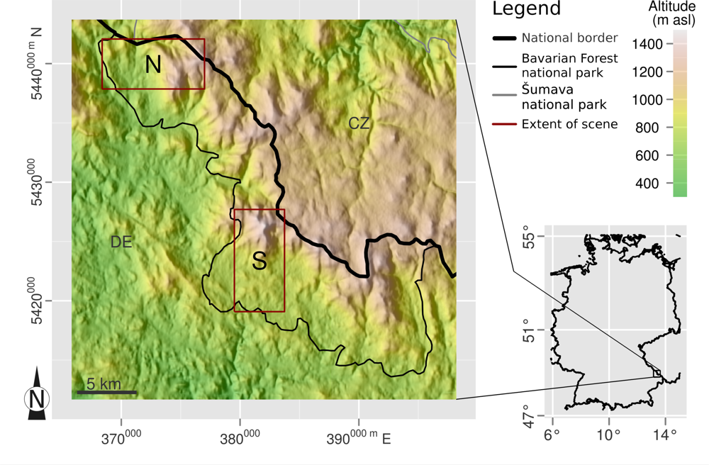
2.1. Study Site
2.2. Remote Sensing Data
2.2.1. Hyperspectral Data
2.2.2. LiDAR
2.3. Biodiversity Data
2.4. Data Preparation
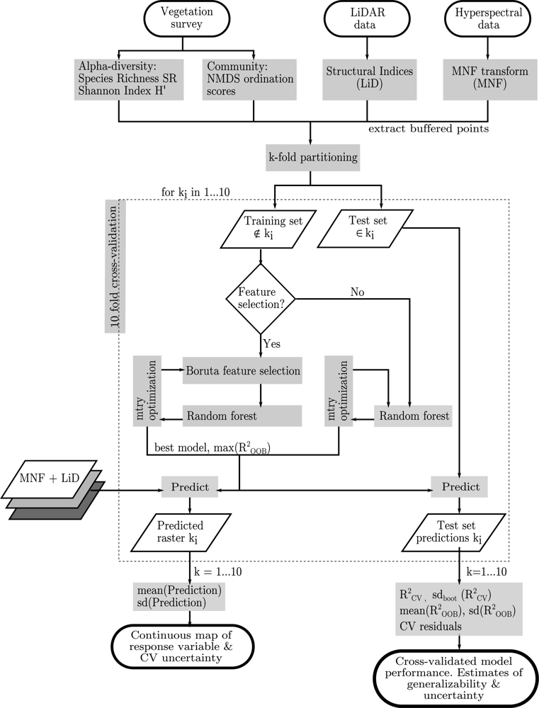
2.5. Statistical Analysis
3. Results
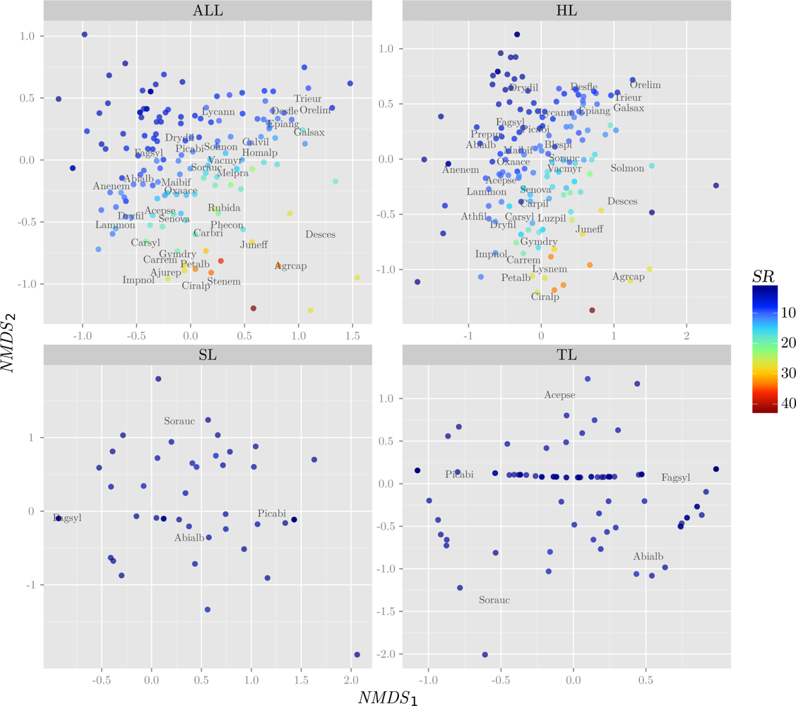
3.1. Response Variables
3.2. Predictor Variables
3.3. Model Fitting
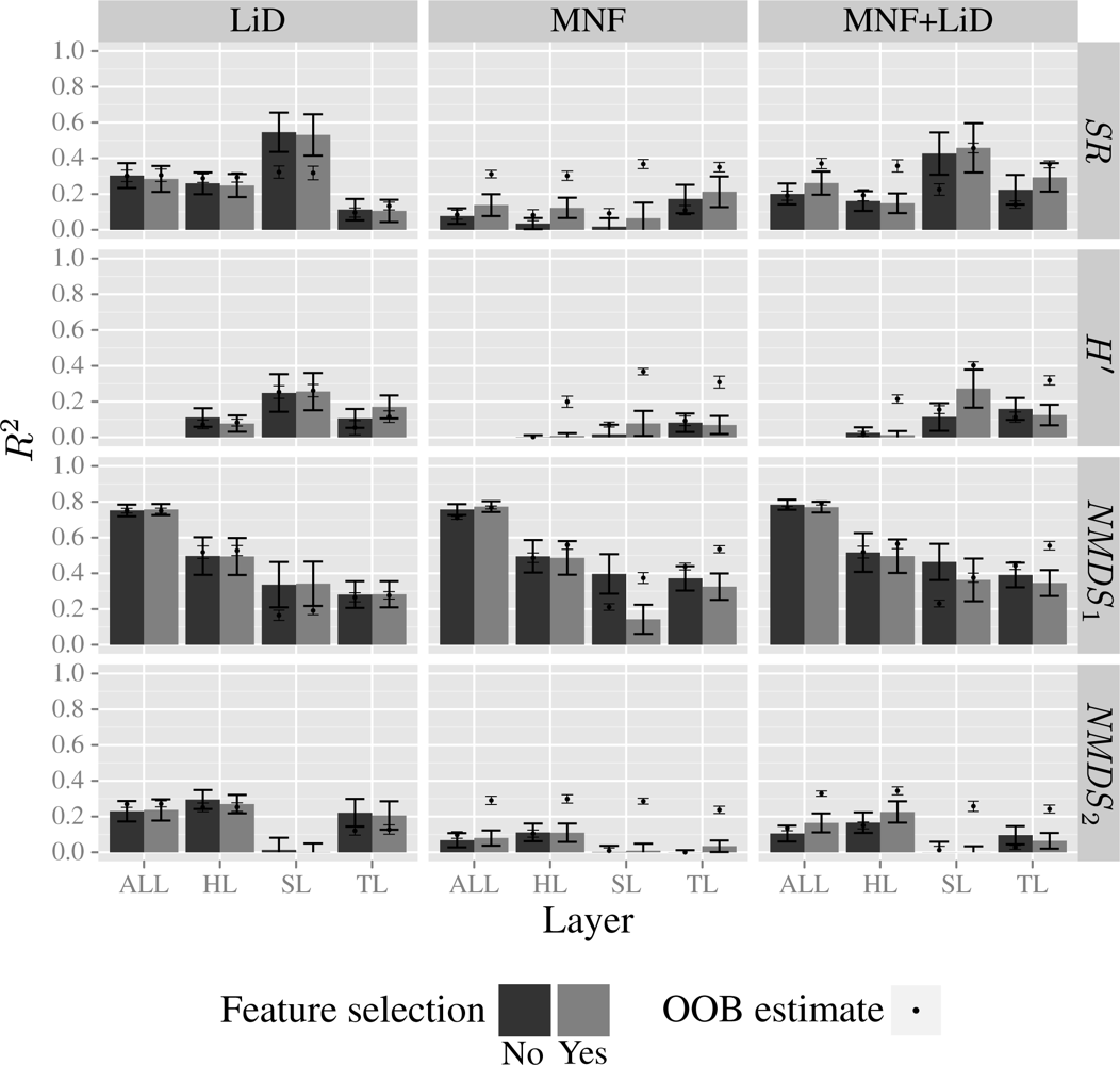
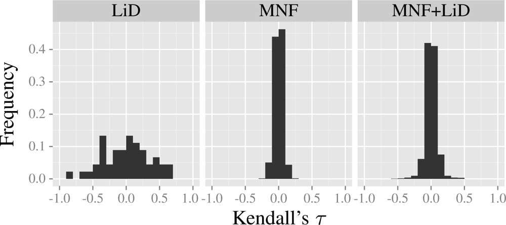
3.4. Model Results
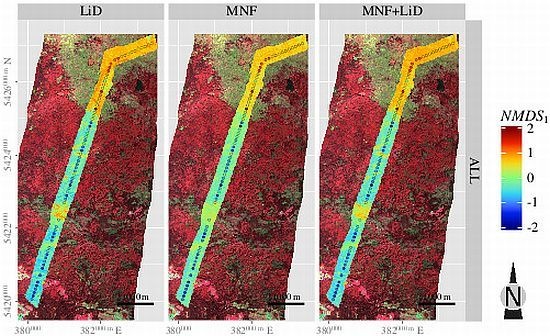
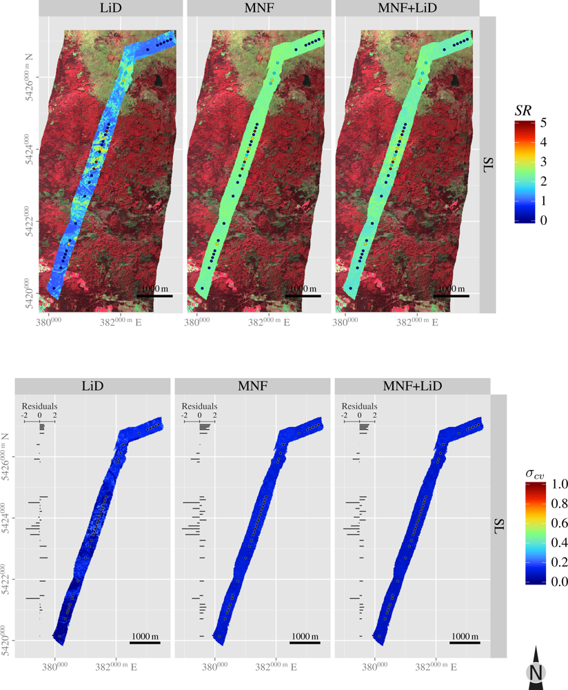
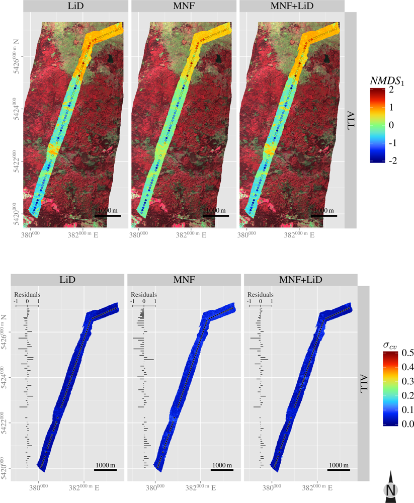
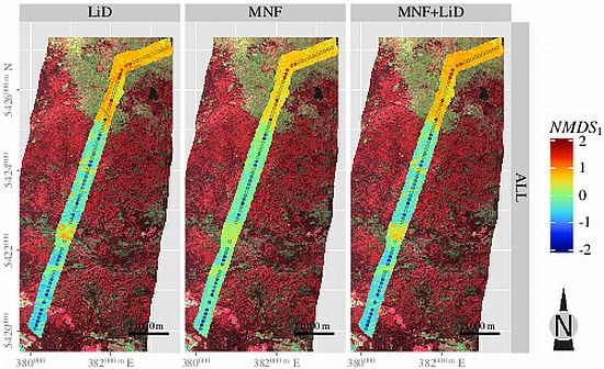
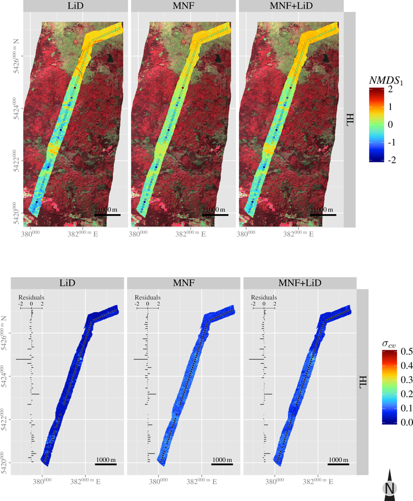
3.5. Spatial Predictions
4. Discussion
5. Conclusions
Acknowledgments
References
- Duffy, J.E. Why biodiversity is important to the functioning of real-world ecosystems. Front. Ecol. Environ 2009, 7, 437–444. [Google Scholar]
- Hector, A.; Bagchi, R. Biodiversity and ecosystem multifunctionality. Nature 2007, 448, 188–190. [Google Scholar]
- Balvanera, P.; Pfisterer, A.B.; Buchmann, N.; He, J.S.; Nakashizuka, T.; Raffaelli, D.; Schmid, B. Quantifying the evidence for biodiversity effects on ecosystem functioning and services. Ecol. Lett 2006, 9, 1146–1156. [Google Scholar] [Green Version]
- Tilman, D.; Reich, P.B.; Knops, J.M.H. Biodiversity and ecosystem stability in a decade-long grassland experiment. Nature 2006, 441, 629–632. [Google Scholar]
- Sala, O.E.; Chapin, F.S.; Armesto, J.J.; Berlow, E.; Bloomfield, J.; Dirzo, R.; Huber-Sanwald, E.; Huenneke, L.F.; Jackson, R.B.; Kinzig, A.; et al. Global biodiversity scenarios for the year 2100. Science 2000, 287, 1770–1774. [Google Scholar]
- Bellard, C.; Bertelsmeier, C.; Leadley, P.; Thuiller, W.; Courchamp, F. Impacts of climate change on the future of biodiversity. Ecol. Lett 2012, 15, 365–377. [Google Scholar]
- United Nations, Convention on Biological Diversity; United Nations: Rio de Janeiro: Brazil, 1992.
- Butchart, S.H.M.; Walpole, M.; Collen, B.; van Strien, A.; Scharlemann, J.P.W.; Almond, R.E.A.; Baillie, J.E.M.; Bomhard, B.; Brown, C.; Bruno, J.; et al. Global biodiversity: Indicators of recent declines. Science 2010, 328, 1164–1168. [Google Scholar]
- Müller, J.; Brandl, R. Assessing biodiversity by remote sensing in mountainous terrain: The potential of LiDAR to predict forest beetle assemblages. J. Appl. Ecol 2009, 46, 897–905. [Google Scholar]
- Turner, W.; Spector, S.; Gardiner, N.; Fladeland, M.; Sterling, E.; Steininger, M. Remote sensing for biodiversity science and conservation. Trends Ecol. Evol 2003, 18, 306–314. [Google Scholar]
- Asner, G.P.; Martin, R.E.; Ford, A.J.; Metcalfe, D.J.; Liddell, M.J. Leaf chemical and spectral diversity in Australian tropical forests. Ecol. Appl 2009, 19, 236–253. [Google Scholar]
- Asner, G.P.; Martin, R.E. Airborne spectranomics: Mapping canopy chemical and taxonomic diversity in tropical forests. Front. Ecol. Environ 2009, 7, 269–276. [Google Scholar]
- Oldeland, J.; Dorigo, W.; Wesuls, D.; Jürgens, N. Mapping bush encroaching species by seasonal differences in hyperspectral imagery. Remote Sens 2010, 2, 1416–1438. [Google Scholar]
- Andrew, M.E.; Wulder, M.A.; Coops, N.C.; Baillargeon, G. Beta-diversity gradients of butterflies along productivity axes. Glob. Ecol. Biogeogr 2012, 21, 352–364. [Google Scholar]
- Hüttich, C.; Gessner, U.; Herold, M.; Strohbach, B.; Schmidt, M.; Keil, M.; Dech, S. On the suitability of MODIS time series metrics to map vegetation types in dry savanna ecosystems: A case study in the Kalahari of NE Namibia. Remote Sens 2009, 1, 620–643. [Google Scholar]
- Cord, A.; Rödder, D. Inclusion of habitat availability in species distribution models through multi-temporal remote-sensing data? Ecol. Appl 2011, 21, 3285–3298. [Google Scholar]
- Vierling, K.; Bässler, C.; Brandl, R.; Vierling, L.; Weiss, I.; Müller, J. Spinning a laser web: Predicting spider distributions using lidar. Ecol. Appl 2011, 21, 577–588. [Google Scholar]
- Bengtsson, J.; Nilsson, S.G.; Franc, A.; Menozzi, P. Biodiversity, disturbances, ecosystem function and management of European forests. For. Ecol. Manage 2000, 132, 39–50. [Google Scholar]
- Feilhauer, H.; Schmidtlein, S. On variable relations between vegetation patterns and canopy reflectance. Ecol. Inform 2011, 6, 83–92. [Google Scholar]
- Rocchini, D.; He, K.S.; Oldeland, J.; Wesuls, D.; Neteler, M. Spectral variation versus species beta-diversity at different spatial scales: A test in African highland savannas. J. Environ. Monit 2010, 12, 825–831. [Google Scholar]
- Oldeland, J.; Wesuls, D.; Rocchini, D.; Schmidt, M.; Jurgens, N. Does using species abundance data improve estimates of species diversity from remotely sensed spectral heterogeneity? Ecol. Indic 2010, 10, 390–396. [Google Scholar]
- Clark, M.L.; Roberts, D.A.; Clark, D.B. Hyperspectral discrimination of tropical rain forest tree species at leaf to crown scales. Remote Sens. Environ 2005, 96, 375–398. [Google Scholar]
- Carlson, K.M.; Asner, G.P.; Hughes, R.F.; Ostertag, R.; Martin, R.E. Hyperspectral remote sensing of canopy biodiversity in Hawaiian lowland rainforests. Ecosystems 2007, 10, 536–549. [Google Scholar]
- Bunting, P.; Lucas, R.M.; Jones, K.; Bean, A.R. Characterisation and mapping of forest communities by clustering individual tree crowns. Remote Sens. Environ 2010, 114, 2536–2547. [Google Scholar]
- Jones, T.G.; Coops, N.C.; Sharma, T. Assessing the utility of airborne hyperspectral and LiDAR data for species distribution mapping in the coastal Pacific Northwest, Canada. Remote Sens. Environ 2010, 114, 2841–2852. [Google Scholar]
- Nagendra, H.; Rocchini, D.; Ghate, R.; Sharma, B.; Pareeth, S. Assessing plant diversity in a dry tropical forest: Comparing the utility of Landsat and IKONOS satellite images. Remote Sens 2010, 2, 478–496. [Google Scholar]
- Clark, M.L. Identification of Canopy Species in Tropical Forests Using Hyperspectral Data. In Hyperspectral Remote Sensing of Vegetation; Thenkabail, P.S., Lyon, J.G., Huete, A., Eds.; CRC Press: Boca Raton, FL, USA, 2012; pp. 423–445. [Google Scholar]
- Gilliam, F.S. The ecological significance of the herbaceous layer in temperate forest ecosystems. BioScience 2007, 57, 845–858. [Google Scholar]
- Wang, K.; Franklin, S.E.; Guo, X.L.; Cattet, M. Remote sensing of ecology, biodiversity and conservation: A review from the perspective of remote sensing specialists. Sensors 2010, 10, 9647–9667. [Google Scholar]
- Bergen, K.M.; Goetz, S.J.; Dubayah, R.O.; Henebry, G.M.; Hunsaker, C.T.; Imhoff, M.L.; Nelson, R.F.; Parker, G.G.; Radeloff, V.C. Remote sensing of vegetation 3-D structure for biodiversity and habitat: Review and implications for lidar and radar spaceborne missions. J. Geophys. Res 2009, 114, G00E06:1–G00E06:13. [Google Scholar]
- Thomas, V. Hyperspectral Remote Sensing for Forest Management. In Hyperspectral Remote Sensing of Vegetation; Thenkabail, P.S., Lyon, J.G., Huete, A., Eds.; CRC Press: Boca Raton, FL, USA, 2012; pp. 469–485. [Google Scholar]
- He, K.S.; Rocchini, D.; Neteler, M.; Nagendra, H. Benefits of hyperspectral remote sensing for tracking plant invasions. Divers. Distrib 2011, 17, 381–392. [Google Scholar]
- Andrew, M.E.; Ustin, S.L. Habitat suitability modelling of an invasive plant with advanced remote sensing data. Divers. Distrib 2009, 15, 627–640. [Google Scholar]
- Plourde, L.C.; Ollinger, S.V.; Smith, M.L.; Martin, M.E. Estimating species abundance in a northern temperate forest using spectral mixture analysis. Photogramm. Eng. Remote Sensing 2007, 73, 829–840. [Google Scholar]
- Schmidtlein, S.; Feilhauer, H.; Bruelheide, H. Mapping plant strategy types using remote sensing. J. Veg. Sci 2012, 23, 395–405. [Google Scholar]
- Rocchini, D.; Ricotta, C.; Chiarucci, A. Using satellite imagery to assess plant species richness: The role of multispectral systems. Appl. Veg. Sci 2007, 10, 325–331. [Google Scholar]
- Feilhauer, H.; Faude, U.; Schmidtlein, S. Combining Isomap ordination and imaging spectroscopy to map continuous floristic gradients in a heterogeneous landscape. Remote Sens. Environ 2011, 115, 2513–2524. [Google Scholar]
- Wang, L.; Sousa, W.P.; Gong, P.; Biging, G.S. Comparison of IKONOS and QuickBird images for mapping mangrove species on the Caribbean coast of Panama. Remote Sens. Environ 2004, 91, 432– 440. [Google Scholar]
- Nagendra, H.; Rocchini, D. High resolution satellite imagery for tropical biodiversity studies: The devil is in the detail. Biodivers. Conserv 2008, 17, 3431–3442. [Google Scholar]
- Schmidtlein, S. Imaging spectroscopy as a tool for mapping Ellenberg indicator values. J. Appl. Ecol 2005, 42, 966–974. [Google Scholar]
- Yue, Y.M.; Wang, K.L.; Zhang, B.; Chen, Z.C.; Jiao, Q.J.; Liu, B.; Chen, H.S. Exploring the relationship between vegetation spectra and eco-geo-environmental conditions in karst region, Southwest China. Environ. Monit. Assess 2010, 160, 157–168. [Google Scholar]
- Bässler, C.; Stadler, J.; Müller, J.; Förster, B.; Göttlein, A.; Brandl, R. LiDAR as a rapid tool to predict forest habitat types in Natura 2000 networks. Biodivers. Conserv 2011, 20, 465–481. [Google Scholar]
- Müller, J.; Stadler, J.; Brandl, R. Composition versus physiognomy of vegetation as predictors of bird assemblages: The role of lidar. Remote Sens. Environ 2010, 114, 490–495. [Google Scholar]
- Müller, J.; Moning, C.; Bässler, C.; Heurich, M.; Brandl, R. Using airborne laser scanning to model potential abundance and assemblages of forest passerines. Basic Appl. Ecol 2009, 10, 671–681. [Google Scholar]
- Goetz, S.; Steinberg, D.; Dubayah, R.; Blair, B. Laser remote sensing of canopy habitat heterogeneity as a predictor of bird species richness in an eastern temperate forest, USA. Remote Sens. Environ 2007, 108, 254–263. [Google Scholar]
- Dalponte, M.; Bruzzone, L.; Gianelle, D. Fusion of hyperspectral and LIDAR remote sensing data for classification of complex forest areas. IEEE Trans. Geosci. Remote Sens 2008, 46, 1416–1427. [Google Scholar]
- Féret, J.B.; Asner, G.P. Semi-supervised methods to identify individual crowns of lowland tropical canopy species using imaging spectroscopy and LiDAR. Remote Sens 2012, 4, 2457–2476. [Google Scholar]
- Stuffler, T.; Kaufmann, C.; Hofer, S.; Förster, K.P.; Schreier, G.; Mueller, A.; Eckardt, A.; Bach, H.; Penné, B.; Benz, U.; Haydn, R. The EnMAP hyperspectral imager—An advanced optical payload for future applications in Earth observation programmes. Acta Astronaut 2007, 61, 115–120. [Google Scholar]
- National Research Council of the National Academiesun, Earth Science and Applications from Space: National Imperatives for the Next Decade and Beyond; National Academies Press: Washington, DC, USA, 2007.
- USGS, Shuttle Radar Topography Mission 3 Arc Second scenes N49E012 and N48E013, v2.1 ed.; Global Land Cover Facility, University of Maryland: College Park, MD, USA, 2006.
- Müller, J.; Bußler, H.; Goßner, M.; Rettelbach, T.; Duelli, P. The European spruce bark beetle Ips typographus in a national park: From pest to keystone species. Biodivers. Conserv 2008, 17, 2979–3001. [Google Scholar]
- Cocks, T.; Jenssen, R.; Stewart, A.; Wilson, I.; Shields, T. The HyMap Airborne Hyperspectral Sensor: The System, Calibration and Performance. Proceedings of the 1st EARSeL Workshop on Imaging Spectroscopy, Zürich, Switzerland, 6–8 October 1998.
- Richter, R.; Schläpfer, D. Geo-atmospheric processing of airborne imaging spectrometry data. Part 2: Atmospheric/topographic correction. Int. J. Remote Sens 2002, 23, 2631–2649. [Google Scholar]
- Green, A.A.; Berman, M.; Switzer, P.; Craig, M.D. A transformation for ordering multispectral data in terms of image quality with implications for noise removal. IEEE Trans. Geosci. Remote Sens 1988, 26, 65–74. [Google Scholar]
- ITT Visual Information Solutions, ENVI 4.7; ITT Visual Information Solutions: Boulder, CO, USA.
- Reitberger, J.; Krystek, P.; Heurich, M. Full-waveform Analysis of Small Footprint Airborne Laser Scanning Data in the Bavarian Forest National Park for Tree Species Classification. Proceedings of the Workshop on 3D Remote Sensing in Forestry, Vienna, Austria, 14–15 February 2006; pp. 218–227.
- Drake, J.B.; Dubayah, R.O.; Clark, D.B.; Knox, R.G.; Blair, J.; Hofton, M.A.; Chazdon, R.L.; Weishampel, J.F.; Prince, S. Estimation of tropical forest structural characteristics using large-footprint lidar. Remote Sens. Environ 2002, 79, 305–319. [Google Scholar]
- Bässler, C.; Förster, B.; Moning, C.; Müller, J. The BIOKLIM Project: Biodiversity research between climate change and wilding in a temperate montane forest-the conceptual framework. Waldoekologie, Landschaftsforschung und Naturschutz 2008, 7, 21–33. [Google Scholar]
- Wyatt, J.L.; Silman, M.R. Centuries-old logging legacy on spatial and temporal patterns in understory herb communities. For. Ecol. Manag 2010, 260, 116–124. [Google Scholar]
- Shepard, R. The analysis of proximities: Multidimensional scaling with an unknown distance function. I. Psychometrika 1962, 27, 125–140. [Google Scholar]
- Kruskal, J. Nonmetric multidimensional scaling: A numerical method. Psychometrika 1964, 29, 115–129. [Google Scholar]
- Foody, G.M.; Cutler, M.E.J. Mapping the species richness and composition of tropical forests from remotely sensed data with neural networks. Ecol. Model 2006, 195, 37–42. [Google Scholar] [Green Version]
- Feilhauer, H.; Asner, G.P.; Martin, R.E.; Schmidtlein, S. Brightness-normalized Partial Least Squares Regression for hyperspectral data. J. Quant. Spectrosc. Radiat. Transf 2010, 111, 1947–1957. [Google Scholar]
- Goetz, S.J.; Steinberg, D.; Betts, M.G.; Holmes, R.T.; Doran, P.J.; Dubayah, R.; Hofton, M. Lidar remote sensing variables predict breeding habitat of a Neotropical migrant bird. Ecology 2010, 91, 1569–1576. [Google Scholar]
- Breiman, L. Random forests. Mach. Learn 2001, 45, 5–32. [Google Scholar]
- Verikas, A.; Gelzinis, A.; Bacauskiene, M. Mining data with random forests: A survey and results of new tests. Pattern Recognit 2011, 44, 330–349. [Google Scholar]
- Kohavi, R. A. Study of Cross-Validation and Bootstrap for Accuracy Estimation and Model Selection. Proceedings of the International Joint Conference on Artificial Intelligence, Montreal, QC, Canada, 20–25 August 1995; pp. 1137–1145.
- Ambroise, C.; McLachlan, G.J. Selection bias in gene extraction on the basis of microarray gene-expression data. Proc. Natl. Acad. Sci. USA 2002, 99, 6562–6566. [Google Scholar]
- Hastie, T.; Tibshirani, R.; Friedman, J. The Elements of Statistical Learning: Data Mining, Inference, and Prediction, Second Edition, 2 ed.; Springer: Berlin/Heidelberg, Germany, 2009. [Google Scholar]
- Kursa, M.B.; Jankowski, A.; Rudnicki, W.R. Boruta-A system for feature selection. Fund. Inform 2010, 101, 271–286. [Google Scholar]
- Cawley, G.C.; Talbot, N.L.C. On over-fitting in model selection and subsequent selection bias in performance evaluation. J. Mach. Learn. Res 2010, 11, 2079–2107. [Google Scholar]
- Genuer, R.; Poggi, J.M.; Tuleau, C. Random Forests: Some Methodological Insights; Technical Report 6729; Institut National de Recherche en Informatique et en Automatique: Paris, France, 2008. [Google Scholar]
- Saeys, Y.; Inza, I.; Larrañaga, P. A review of feature selection techniques in bioinformatics. Bioinformatics 2007, 23, 2507–2517. [Google Scholar]
- Hua, J.; Xiong, Z.; Lowey, J.; Suh, E.; Dougherty, E.R. Optimal number of features as a function of sample size for various classification rules. Bioinformatics 2004, 21, 1509–1515. [Google Scholar]
- R Development Core Team, R: A Language and Environment for Statistical Computing; R Foundation for Statistical Computing: Vienna, Austria, 2012.
- Oksanen, J.; Blanchet, F.G.; Kindt, R.; Legendre, P.; Minchin, P.R.; O’Hara, R.B.; Simpson, G.L.; Solymos, P.; Stevens, M.H.H.; Wagner, H. Vegan: Community Ecology Package. 2012. Available online: http://CRAN.R-project.org/package=vegan (accessed on 20 September 2012).
- Liaw, A.; Wiener, M. Classification and regression by randomForest. R News 2002, 2, 18–22. [Google Scholar]
- Kursa, M.B.; Rudnicki, W.R. Feature selection with the boruta package. J. Stat. Softw 2010, 36, 1–13. [Google Scholar]
- Wickham, H. Ggplot2: Elegant Graphics for Data Analysis; Springer: New York, NY, USA, 2009. [Google Scholar]
- Landolt, E.; et al. Flora Indicativa: Ecological Indicator Values and Biological Attributes of the Flora of Switzerland and the Alps; Editions des Conservatoire et Jardin Botaniques de la Ville de Genève; WSL: Lausanne, Switzerland, 2010; Volume 2, p. 376. [Google Scholar]
- Rocchini, D.; Balkenhol, N.; Carter, G.A.; Foody, G.M.; Gillespie, T.W.; He, K.S.; Kark, S.; Levin, N.; Lucas, K.; Luoto, M.; et al. Remotely sensed spectral heterogeneity as a proxy of species diversity: Recent advances and open challenges. Ecol. Inform 2010, 5, 318–329. [Google Scholar]
- Vockenhuber, E.A.; Scherber, C.; Langenbruch, C.; Meissner, M.; Seidel, D.; Tscharntke, T. Tree diversity and environmental context predict herb species richness and cover in Germany’s largest connected deciduous forest. Perspect. Plant Ecol. Evol. Syst 2011, 13, 111–119. [Google Scholar]
- Falkowski, M.J.; Evans, J.S.; Martinuzzi, S.; Gessler, P.E.; Hudak, A.T. Characterizing forest succession with lidar data: An evaluation for the Inland Northwest, USA. Remote Sens. Environ 2009, 113, 946–956. [Google Scholar]
- Lefsky, M.; Cohen, W.; Spies, T. An evaluation of alternate remote sensing products for forest inventory, monitoring, and mapping of Douglas-fir forests in western Oregon. Can. J. For. Res 2001, 31, 78–87. [Google Scholar]
- Schmidtlein, S.; Zimmermann, P.; Schüpferling, R.; Weiß, C. Mapping the floristic continuum: Ordination space position estimated from imaging spectroscopy. J. Veg. Sci 2007, 18, 131–140. [Google Scholar]
- Mundt, J.T.; Streutker, D.R.; Glenn, N.F. Mapping sagebrush distribution using fusion of hyperspectral and lidar classifications. Photogramm. Eng. Remote Sensing 2006, 72, 47–54. [Google Scholar]
- Onojeghuo, A.O.; Blackburn, G.A. Optimising the use of hyperspectral and LiDAR data for mapping reedbed habitats. Remote Sens. Environ 2011, 115, 2025–2034. [Google Scholar]
- Hassler, S.K.; Kreyling, J.; Beierkuhnlein, C.; Eisold, J.; Samimi, C.; Wagenseil, H.; Jentsch, A. Vegetation pattern divergence between dry and wet season in a semiarid savanna-Spatio-temporal dynamics of plant diversity in northwest Namibia. J. Arid Environ 2010, 74, 1516–1524. [Google Scholar]
- Tuomisto, H. A diversity of beta diversities: Straightening up a concept gone awry. Part 1. Defining beta diversity as a function of alpha and gamma diversity. Ecography 2010, 33, 2–22. [Google Scholar]
- Jurasinski, G.; Retzer, V.; Beierkuhnlein, C. Inventory, differentiation, and proportional diversity: A consistent terminology for quantifying species diversity. Oecologia 2009, 159, 15–26. [Google Scholar]
- Jurasinski, G.; Jentsch, A.; Retzer, V.; Beierkuhnlein, C. Detecting spatial patterns in species composition with multiple plot similarity coefficients and singularity measures. Ecography 2012, 35, 73–88. [Google Scholar]
- Baselga, A.; Jimenez-Valverde, A.; Niccolini, G. A multiple-site similarity measure independent of richness. Biol. Lett 2007, 3, 642–645. [Google Scholar]
- Steinbauer, M.; Dolos, K.; Reineking, B.; Beierkuhnlein, C. Current measures for distance decay in similarity of species composition are influenced by study extent and grain size. Glob. Ecol. Biogeogr 2012. accepted. [Google Scholar]
- Qian, H.; Ricklefs, R.E. Disentangling the effects of geographic distance and environmental dissimilarity on global patterns of species turnover. Glob. Ecol. Biogeogr 2012, 21, 341–351. [Google Scholar]
- Diaz-Uriarte, R.; Alvarez de Andres, S. Gene selection and classification of microarray data using random forest. BMC Bioinforma 2006, 7, 3:1–3:13. [Google Scholar]
- Strobl, C.; Boulesteix, A.L.; Kneib, T.; Augustin, T.; Zeileis, A. Conditional variable importance for random forests. BMC Bioinforma 2008, 9, 307. [Google Scholar]
- Harrel, F.E. Regression Modeling Strategies–with Applications to Linear Models, Logistic Regression, and Survival Analysis; Springer: Berlin/Heidelberg, Germany, 2001; p. 570. [Google Scholar]
- Dormann, C.F.; Elith, J.; Bacher, S.; Buchmann, C.; Carl, G.; Carré, G.; Marquéz, J.R.G.; Gruber, B.; Lafourcade, B.; Leitão, P.J.; et al. Collinearity: A review of methods to deal with it and a simulation study evaluating their performance. Ecography 2012, in press. [Google Scholar]
- Dudoit, S.; Fridlyand, J.; Speed, T. Comparison of discrimination methods for the classification of tumors using gene expression data. J. Am. Stat. Assoc 2002, 97, 77–87. [Google Scholar]
- Hofer, G.; Wagner, H.H.; Herzog, F.; Edwards, P.J. Effects of topographic variability on the scaling of plant species richness in gradient dominated landscapes. Ecography 2008, 31, 131–139. [Google Scholar]
- Leutner, B.; Steinbauer, M.; Müller, C.; Früh, A.; Irl, S.; Jentsch, A.; Beierkuhnlein, C. Mosses like it rough—Growth form specific responses of mosses, herbaceous and woody plants to micro-relief heterogeneity. Diversity 2012, 4, 59–73. [Google Scholar]
- Böhner, J.; Selige, T. Spatial prediction of soil attributes using terrain analysis and climate regionalisation. Gött. Geogr. Abh 2006, 115, 13–27. [Google Scholar]
- Xiao, Y.; Segal, M.R. Identification of yeast transcriptional regulation networks using multivariate random forests. PLoS Comput. Biol 2009, 5, e1000414:1–e1000414:18. [Google Scholar]


| Layer | H′ | NMDS1 | NMDS2 | |
|---|---|---|---|---|
| ALL | SR | 0.3 | –0.6 | |
| NMDS1 | 0.0 | |||
| HL | SR | 0.5 | 0.3 | –0.5 |
| H′ | 0.0 | –0.4 | ||
| NMDS1 | 0.0 | |||
| SL | SR | 0.9 | 0.3 | 0.1 |
| H′ | 0.3 | 0.1 | ||
| NMDS1 | –0.2 | |||
| TL | SR | 0.8 | 0.0 | –0.4 |
| H′ | –0.0 | –0.4 | ||
| NMDS1 | 0.0 | |||
Share and Cite
Leutner, B.F.; Reineking, B.; Müller, J.; Bachmann, M.; Beierkuhnlein, C.; Dech, S.; Wegmann, M. Modelling Forest α-Diversity and Floristic Composition — On the Added Value of LiDAR plus Hyperspectral Remote Sensing. Remote Sens. 2012, 4, 2818-2845. https://doi.org/10.3390/rs4092818
Leutner BF, Reineking B, Müller J, Bachmann M, Beierkuhnlein C, Dech S, Wegmann M. Modelling Forest α-Diversity and Floristic Composition — On the Added Value of LiDAR plus Hyperspectral Remote Sensing. Remote Sensing. 2012; 4(9):2818-2845. https://doi.org/10.3390/rs4092818
Chicago/Turabian StyleLeutner, Benjamin F., Björn Reineking, Jörg Müller, Martin Bachmann, Carl Beierkuhnlein, Stefan Dech, and Martin Wegmann. 2012. "Modelling Forest α-Diversity and Floristic Composition — On the Added Value of LiDAR plus Hyperspectral Remote Sensing" Remote Sensing 4, no. 9: 2818-2845. https://doi.org/10.3390/rs4092818