Application of a Remote Sensing Method for Estimating Monthly Blue Water Evapotranspiration in Irrigated Agriculture

 ,
,
Abstract
: In this paper we show the potential of combining actual evapotranspiration (ETactual) series obtained from remote sensing and land surface modelling, to monitor community practice in irrigation at a monthly scale. This study estimates blue water evapotranspiration (ETb) in irrigated agriculture in two study areas: the Horn of Africa (2010–2012) and the province of Sichuan (China) (2001–2010). Both areas were affected by a drought event during the period of analysis, but are different in terms of water control and storage infrastructure. The monthly ETb results were separated by water source—surface water, groundwater or conjunctive use—based on the Global Irrigated Area Map and were analyzed per country/province. The preliminary results show that the temporal signature of the total ETb allows seasonal patterns to be distinguished within a year and inter-annual ETb dynamics. In Ethiopia, ETb decreased during the dry year, which suggests that less irrigation water was applied. Moreover, an increase of groundwater use was observed at the expense of surface water use. In Sichuan province, ETb in the dry year was of similar magnitude to the previous years or increased, especially in the month of August, which points to a higher amount of irrigation water used. This could be explained by the existence of infrastructure for water storage and water availability, in particular surface water. The application presented in this paper is innovative and has the potential to assess the existence of irrigation, the source of irrigation water, the duration and variability in time, at pixel and country scales, and is especially useful to monitor irrigation practice during periods of drought.1. Introduction
The assessment of water use is crucial in a changing environment in which water is an essential but scarce resource. From a water management perspective, an accurate evaluation of the irrigation water used in agriculture is of high importance. The AQUASTAT database [1] shows a wide range of values on water withdrawal for irrigation, with values ranging for example from 0.6% of total national water withdrawal in the Netherlands to 60% or 85% in Spain and Tanzania, respectively.
Crop water use or evapotranspiration (ETactual) has traditionally been separated into a “green” and “blue” component, referring to the origin of the used water: precipitation or irrigation water, respectively. Early studies estimated blue and/or green water use at country, continental or global levels [2–5]. Later studies made global estimates of consumptive water use for a number of specific crops per country [6–9]. At a global scale and higher spatial resolution, Alcamo et al. [10] estimated blue water withdrawal and Döll and Siebert [11] the irrigation water requirements. More recently, a few studies estimated global green and blue water consumption in crop production at spatial resolutions of 30 and 5 arc minutes [12–20].
The aforementioned approaches used hydrological models with the objective of estimating actual evapotranspiration from croplands per crop type, distinguishing between blue and green ETactual. However, the input used and the type of output produced, differed. The results were calculated and presented at different spatial resolutions and covered different time periods. The inputs of the methods were national statistics, reports, climatic databases and crop-related maps. The spatial and temporal resolutions of the source data were coarse in some cases, especially where extracted from statistical databases, implying in some cases the use of disaggregation techniques.
Bearing this in mind, remote sensing techniques may improve the estimates of blue and green water use since they provide global coverage, varied temporal and spatial resolution and broad spectral information. This allows characterizing the physical processes and monitoring crops in appropriate space and time scales. In this context, Romaguera et al. [21,22] included the use of remote sensing data and proposed a methodology to estimate blue water evapotranspiration (ETb) that could benefit from the remote sensing advantages. This method allows the estimation of ETb at different time scales, i.e., hourly, daily, monthly and yearly, which is supposedly an improvement with respect to the existing static maps for monitoring irrigation practice. At regional scale, other works used remote sensing to evaluate irrigation performance [23–25].
Moreover, in recent years, several studies have approached the problem of global irrigation mapping, using national statistical data as input [26,27] or making use of spectral and temporal remote sensing data to perform classifications and obtain irrigated areas [28,29]. These methods provide information about areas equipped for irrigation, about crop dominance and irrigation source, and about existence or absence of irrigation, but none of the methods quantifies the actual amount of water received by the crops through irrigation, or blue water. In particular, the source of irrigation water was determined by Thenkabail et al. [29,30] in their Global Irrigated Area Map (GIAM), where irrigated areas were classified as a function of three sources of irrigation supply: surface water, groundwater, and conjunctive use (due to usage of stored rain water).
The objective of this paper is to apply the remote sensing method by Romaguera et al. [21,22] and obtain ETb values at relevant time scales for water management purposes, that is at monthly and country/province scale, as well as to show preliminary results and the potential of exploiting these data when combined with the source of irrigation water, from the aforementioned GIAM map. The regions and period of study are the Horn of Africa (period 2010–2012) and the Chinese province of Sichuan (period 2001–2010), both affected by a drought event during the period of study, but with differences in terms of water control and storage infrastructure.
Section 2 describes the method and datasets used in this paper and Section 3 the selected study areas. Section 4 includes ETb time series per source of irrigation water in the study areas and a sensitivity analysis. Section 5 discusses relevant aspects of the application tackled in this research and finally the conclusions of this work are summarized.
2. Method and Data
The method to estimate ETb used in this paper is described in Romaguera et al. [21,22]. It is based on the calculation of the differences in actual evapotranspiration (ETactual) given by remotely sensed ETactual data (RS–ET in the following) and the Global Land Data Assimilation System (GLDAS) ETactual model simulations (GLDAS–ET in the following). The former included the effect of irrigation where relevant, whereas irrigation was not incorporated in GLDAS simulations. A bias between the two datasets is calculated in rain-fed croplands, where no irrigation is supplied, and then used to correct the whole dataset, obtaining ETb as:
2.1. Bias Estimation
Since the two datasets present systematic discrepancies, rain-fed croplands were used to calculate a reference bias to correct for this effect and isolate the differences due to irrigation practices. The GlobCover land cover map (version 2.3) [32] was used to identify rain-fed croplands.
Previous literature showed temporal and spatial variations of this bias [21,33]. For example, in Europe the bias amplitude changed through the year roughly resembling a positive concave curve. The maximum amplitude value reached up to 3 mm/day and occurred in the months of spring and summer in northern latitudes [21]. In that paper, the spatial variability of the bias was taken into account by performing a classification of the study area and calculating the spatial mean bias per class and per month. Normalized Difference Vegetation Index (NDVI) and satellite observation angle were the input parameters for the classification. The validity of the bias curves obtained was carried out by analyzing their representativeness in bigger areas, providing satisfactory results in majority classes.
The classification scheme was improved in recent literature [22] by testing different classification approaches and proposing a new set of input parameters. This allowed to obtain a better differentiation of the bias curves, reduced the standard deviation of the data and captured the expected variability of the maximum bias.
Therefore, following Romaguera et al. [22], in the present work a yearly classification of every study area was carried out with the k-means algorithm and using the following parameters as inputs: a yearly climatic indicator (CI) based on net radiation and precipitation, the maximum value of monthly ETactual along the year (ETmmax), the month where the ETmmax occurs (t_ETmmax) and the maximum NDVI (NDVImax) in the year of interest. The optimal number of classes was calculated using a scattering distance (SD) quality index [34].
For every year and area, a classification was generated and biases per month were obtained by spatially averaging the bias obtained in rain-fed croplands per class. Finally, Equation (1) was used in the study areas to calculate the total ETb per month and the GIAM map to assign the source of irrigation water per pixel.
2.2. Data
Table 1 describes the main characteristics of the datasets used in the present work which are detailed in the following paragraphs.
Remote sensing ETactual estimates were obtained from two sources: the Meteosat Second Generation products provided by the Land Surface Analysis–Satellite Applications Facility (LSA–SAF) [35] for the region of Africa (period 2010–2012) and the dataset produced by Chen et al. [36,37] over China during the years 2001 till 2010. The periods of study and areas were (partially) determined by the availability of data at the moment of writing this paper. The inclusion of the region of China allowed the analysis of a longer time series of data, which was limited in the Meteosat products over Africa, and also allowed the estimation of ETb in a region with more extensive irrigation practices and infrastructure, which is China.
The MSG ETactual model is a simplified Soil–Vegetation–Atmosphere Transfer (SVAT) scheme that uses as input a combination of remote sensed data and atmospheric model outputs. The inputs based on remote sensing are LSA–SAF products of albedo, and downwelling short and longwave radiation fluxes [35,38].The dataset from Chen et al. [37] is based on the Surface Energy Balance System (SEBS) [39], which uses multi-sensor remote sensing based NDVI, albedo, surface emissivity and temperature.
Simulated ETactual data with the Noah model [40] were acquired from the Global Land Data Assimilation System (GLDAS) [41]. The Noah land surface model is a 1D column model that describes the physical processes of the soil, vegetation and snowpack. The inputs of this model are satellite and ground-based observational data. The calculation of the latent (LE) and sensible (H) heat flux start from potential LE (LEp), based on the soil moisture, atmosphere states, and vegetation characteristics. Constrains to LEp are applied resulting in the actual LE and ETactual.
The GlobCover land cover map (version 2.3) [32] was used to identify rain-fed croplands. This map is based on classification techniques which use the surface reflectance observed by the Medium Resolution Imaging Spectrometer (MERIS).
The inputs for the classification of the study areas were obtained from the following sources. Net radiation (Rn) (as a sum of longwave and shortwave radiation) and precipitation (P) (as a sum of rainfall and snowfall rate) were also taken from the GLDAS dataset. These were used to calculate the climatic indicator as the ratio LP/Rn, where L(J/kg) is the latent heat of vaporization, P (mm) is the annual precipitation and Rn (W/m2) is the annual net radiation. The monthly ETactual used for the classification was taken from GLDAS. Data on NDVI was obtained from the Advanced Very High Resolution Radiometer (AVHRR) delivered by the Deutsches Zentrum für Luft- und Raumfahrt (DLR) and from the Satellite Pour l’Observation de la Terre (SPOT–Vegetation). These NDVI sources were selected as inputs for the classification because they are the ones used for the RS–ET estimations, and their values may influence the differences/biases between RS–ET and model simulations.
The Global Irrigated Area Map by Thenkabail et al. [30] was used to identify the source of irrigation, i.e., surface water, groundwater or conjunctive use. This map shows global irrigated areas and classifies them depending on the type of irrigation. The “surface water” (SW) class includes major and medium irrigation from surface water based on large and medium dams. The “groundwater” (GW) class describes minor irrigation from groundwater, small reservoirs and tanks. The “conjunctive use” (CU) class comprises predominately minor irrigation from groundwater, small reservoirs and tanks, but with some mix of surface water irrigation from major reservoirs. This map was generated using classification techniques whose input data were remote sensing based reflectivity, NDVI, rainfall, tree cover and elevation, combined with ground data and Google Earth imagery.
From a technical point of view the inputs were resampled to a common grid and projection, and the resolution of remote sensing data was chosen to calculate the ETb results, that is 0.030 and 0.1 degree for the Horn of Africa and the Chinese region respectively. The separation of SW, GW and CU was carried out at the resolution of the GIAM map, which is 10 km. The temporal resolution of a month was chosen in this analysis. In order to homogenize the data, daily ETactual values from MSG were monthly aggregated.
3. Study Areas
Based on the availability of remote sensing data, two study areas, both affected by a drought event during the period of study, but with differences in terms of water control/storage infrastructure were selected. First, the Horn of Africa was affected by a drought in the year 2011 [42,43]. In particular, Ethiopia is considered a water scarce country. Despite the abundance of water in some parts of the country (central, western and southwestern parts), the distribution and availability of water is erratic both in space and time due to the lack of water control/storage infrastructures [44]. Strategies have been implemented at national level to improve in this direction, like the Irrigation and Drainage Project [45].
Secondly, China is a country with abundant water resources where dams and reservoirs are numerous, built for hydropower generation, flood control, irrigation and drought mitigation. In particular, in the province of Sichuan we can find the Dujiangyan irrigation project [46], a more than 2000 year old system that was developed to prevent flood and nowadays is crucial in draining off flood water, irrigating farms and provide water resources for more than 50 cities in the province. This region suffered a severe drought in 2006 [47,48].
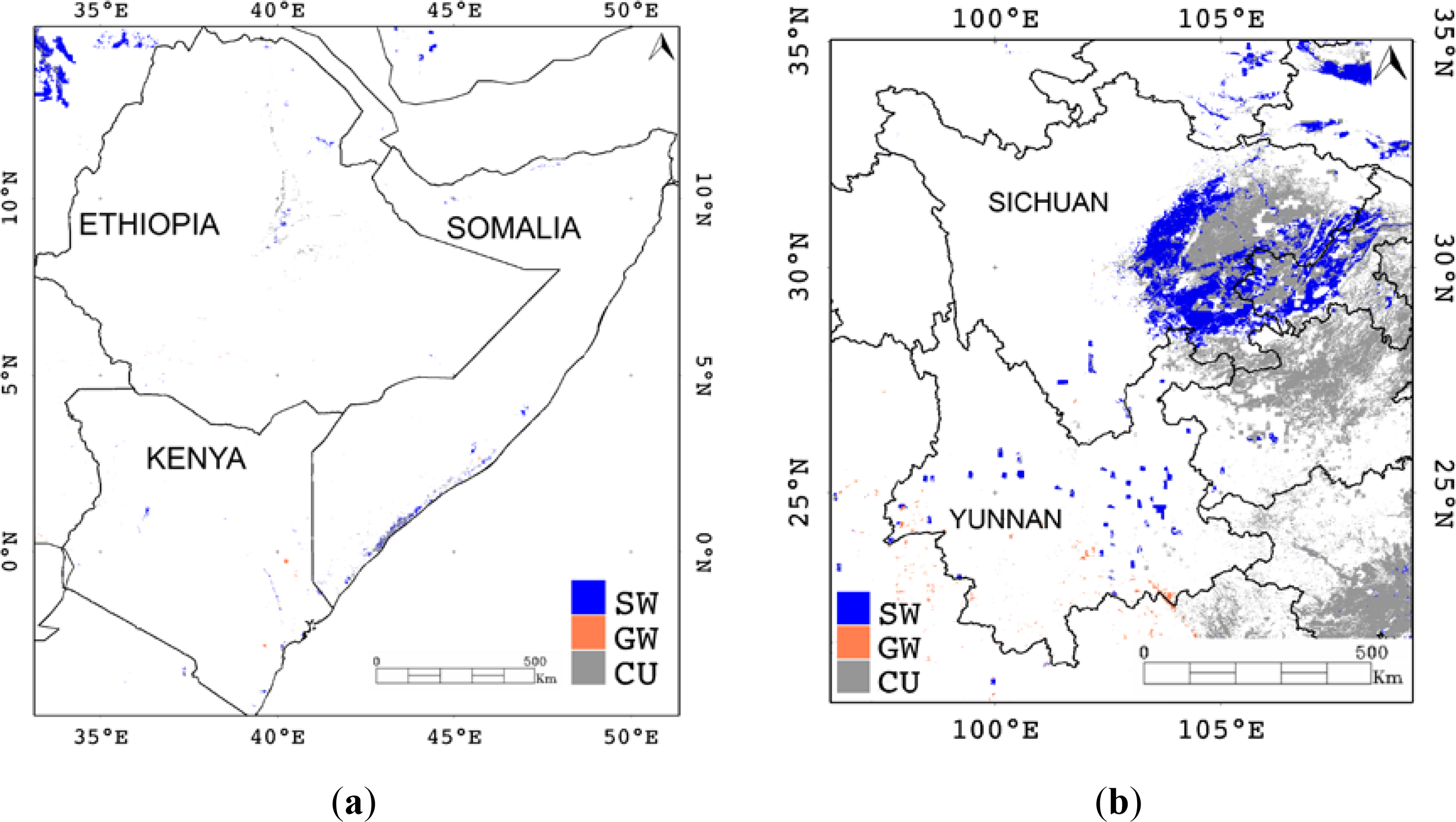
Figure 1 shows the GIAM map, location and size of the study areas. For the sake of comparison, the neighboring countries/provinces were included in the study area, which computed a total of 1,680,000 and 875,000 km2 in the regions of East Africa and Southwest of China respectively. Based on this map, irrigated areas were scarce in the Horn of Africa, mainly concentrated in the center and middle-north of Ethiopia, middle-west and southeast of Kenya and in the coastal areas of south Somalia. In Sichuan province, irrigated areas were abundant in the eastern part and they were scattered in Yunnan province.
4. Results
4.1. Bias Curves
The spatial distribution of the bias was obtained monthly for every study area (not shown here). These computed a total of 36 images in the Horn of Africa, and 120 in the Chinese area, for the time periods analyzed (three and 10 years respectively). After the classification of the study areas, the monthly bias value was obtained per class by averaging the monthly biases in rain-fed croplands.
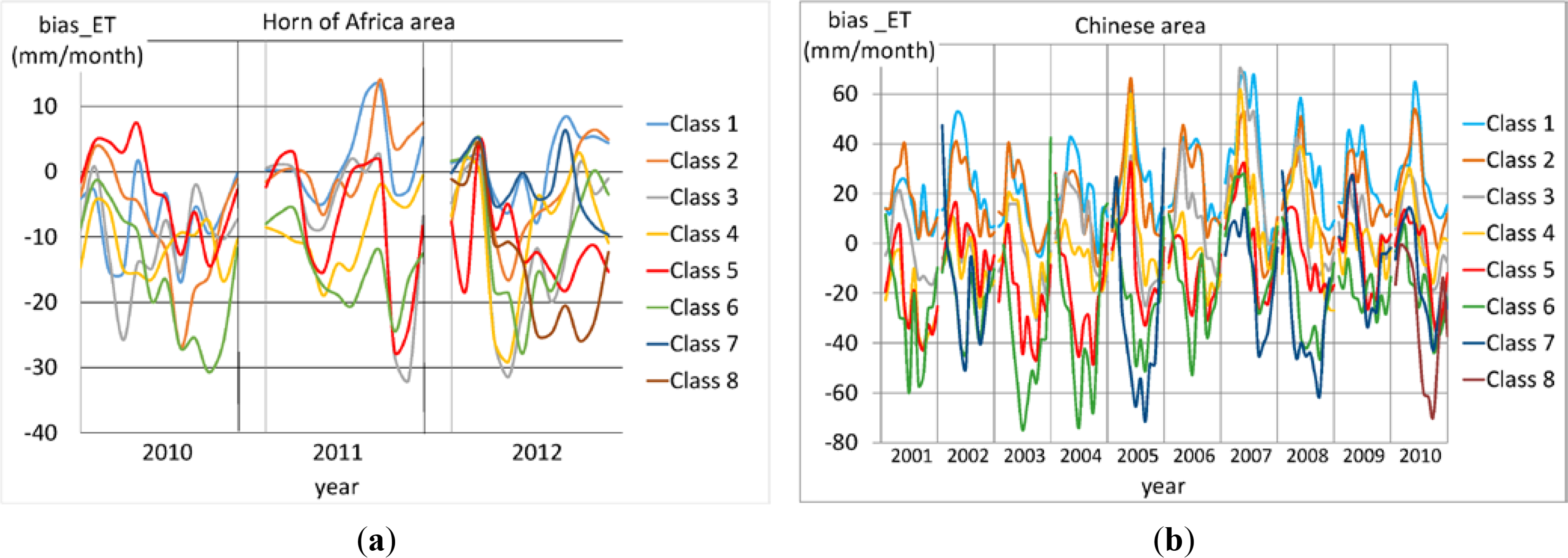
Figure 2 shows the inter-annual variability of the resulting bias curves. The yearly classification of the study areas provided the following number of classes: six (for 2010 and 2011) and eight (for 2012) in the Horn of Africa; six (for 2001, 2003, 2004, 2006), seven (for 2002, 2005, 2007, 2008, 2009) and eight (for 2010) in the Chinese area. In general, largest biases and similar patterns over the years were found in the Southwest of China, with amplitudes between −80 and 80 mm/month. The largest biases were found for the years 2005 and 2010, and the lowest biases for 2009.
The bias curves found in the Horn of Africa show no clear pattern over the years for some classes, which may be explained by the relatively low number of rain-fed pixels used to obtain them. This is the case of classes 1 and 2 in 2010 and class 1 in 2011, where the number of pixels used is one or two orders of magnitude lower than the rest of the classes. Moreover, in some classes the absence of a clear centered peak as observed in China is related to the incoming solar radiation patterns at these latitudes (between 5°S and 15°N). At the equator, maximum radiation values are found at the equinoxes (March and September) and a single maximum is developed with increasing latitude. In this paper, the biases were calculated as spatial averages per class, therefore the combination of values from different latitudes may partially explain the fluctuations of the curves.
For all classes, the magnitude of the biases in the African region is relatively modest compared to the ones found in the region of China. As a reference, we provide the average monthly ETactual in both regions for the year 2010 obtained from the GLDAS–ET data set. The value was computed over all land pixels shown in Figure 1. The average monthly ETactual ranged from 25–60 mm/month and from 25–120 mm/month in the African and Chinese regions respectively. These differences can partly explain the magnitude of the amplitudes found in the bias curves.
4.2. Monthly ETb and Source of Irrigation
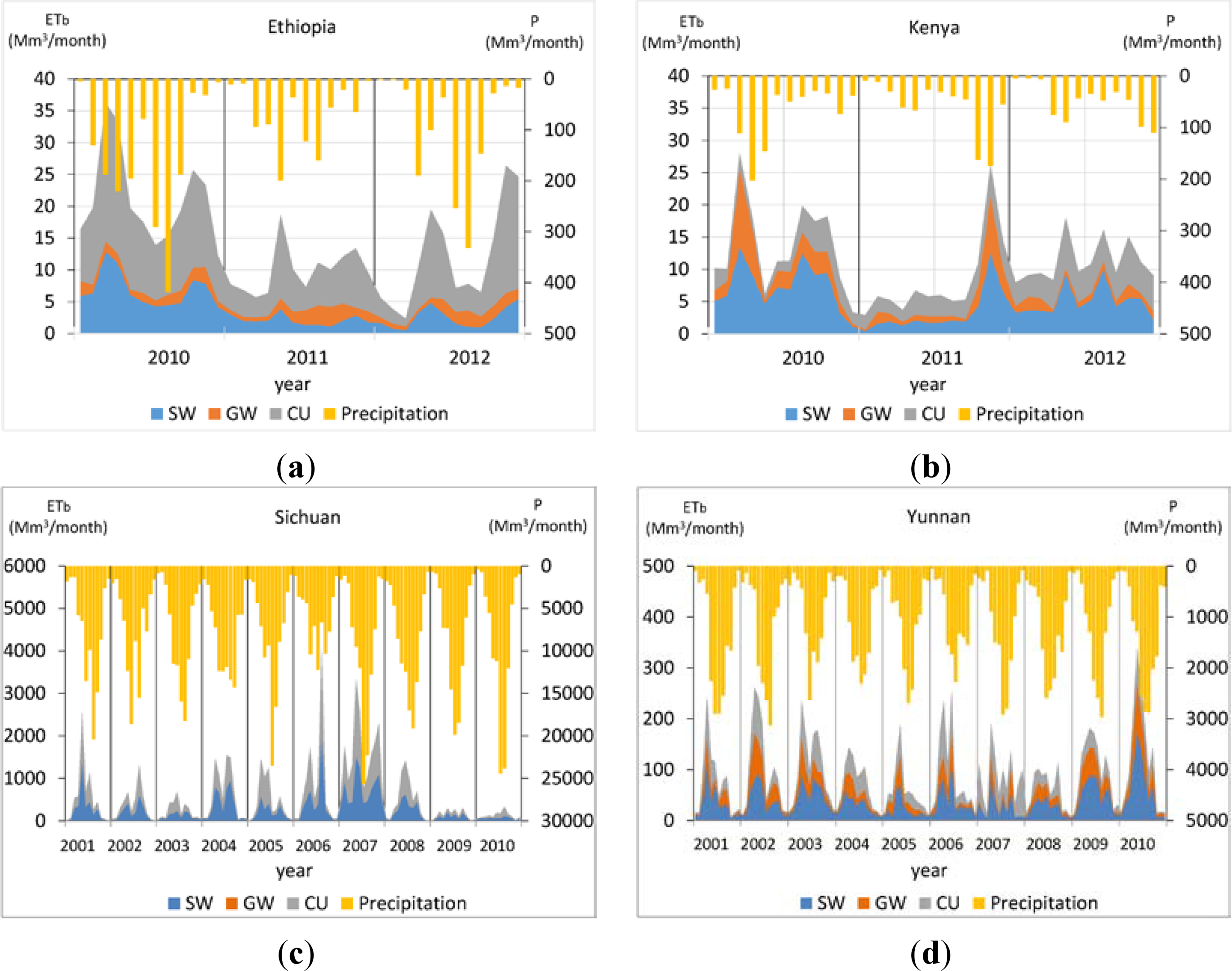
This section contains preliminary results of the application of the ETb method in the study areas. Monthly ETb was calculated for the Horn of Africa for the period 2010 till 2012 and for the Southwest of China for the years 2001–2010. Monthly ETb values were extracted from the pixels labeled by GIAM as irrigated and assigned to the corresponding source of irrigation (SW, GW, CU). Pixel values were converted to volumes (Mm3/month) by using the pixel area and then aggregated per country/province. Figure 3 shows the first results in the study areas where the monthly values of precipitation aggregated over the evaluated pixels are also included.
The temporal signature of ETb allows seasonal patterns to be distinguished within a year and also inter-annual ETb dynamics, especially in the long series of ETb obtained in the provinces of China. The ETb pattern in Yunnan province was found to be relatively regular, contrary to what was observed in Sichuan, with some ETb peaks in the years 2006 and 2007 and lower general values in 2009 and 2010.
Precipitation showed a significant decrease in the year 2011 in Ethiopia and in the year 2006 in Sichuan province. This corresponds to drought periods as explained in Section 3.
In Ethiopia, a general decrease of ETb was observed in 2011, which points at a lower amount of irrigation water used. In particular, total ETb was estimated to decrease from 21 Mm3/month in the wet year 2010 to 10 Mm3/month in the dry year 2011. Moreover, in this period an increase of groundwater use at the expense of surface water use was observed, which is consistent with the report by Hendrix [49]. Despite the existence of the drought, national crop production did not appear to be significantly affected as reported by the Food and Agriculture Organization of the United Nations [50]. This might be explained by the fact that the drought mainly affected the east and south of the country and the majority of croplands use rain-fed production systems and are located in the other part of the country [51].
A decrease of ETb in half of the year 2011 was also observed in Kenya. The precipitation values in this period were only slightly lower than for other years. The drought in Kenya affected the northeastern regions of the country and therefore there is no significant effect on the precipitation in irrigated areas. The study of longer time series of data would allow inter-annual variability, trends and anomalies to be analyzed with a better statistical representation, and therefore have a better interpretation of these patterns.
In Sichuan province, the values of ETb in the dry year were of similar magnitude to the previous years or increased, especially in the month of August, which points to a higher amount of irrigation water used. In particular, ETb was estimated at 200 Mm3/month in the wet year 2005 and 400 Mm3/month in the dry year 2006. The National Bureau of Statistics of China [52] reported that total water resources in Sichuan decreased by 26% in 2006 with respect to the average of other reported years (2004–2012), but still with a high value of 187 billion m3. Moreover, the grain production in 2006 was only 10% lower than in year 2005. These two facts suggest that water was still available for irrigation and it was used when precipitation decreased.
In order to better interpret the results obtained, Figure 4 shows the input RS–ET and GLDAS–ET values in August 2006, where a peak of ETb is found in Sichuan. In this study area the range of RS–ET values was double the ones given by the land surface model in GLDAS–ET, with values up to 330 mm/month. In particular, a hot spot was found in Sichuan province near the border with Chongqing province with low values of GLDAS–ET. There is a high density of irrigated agriculture in this area (see Figure 1), so that the aggregated results per province are highly influenced by these values. Figure 4 also includes the temporal series of these two ETactual estimates in a pixel of the hot spot, where the significant decrease of GLDAS–ET outputs in the year 2006 can be observed. Due to the lack of precipitation, the ETactual model outputs given by the land surface model are lower.
In Yunnan province, in which there was no significant dry year during the period of analysis, the total ETb curves show relatively regular patterns and values ten times smaller than in Sichuan. The use of the three sources of irrigation water is observed in this province with a major use of surface water.
In general, the preliminary results shown in Figure 3 also reveal features that could not be explained, like the ETb peaks in Sichuan in 2007 or low ETb values in 2009 and 2010. Although further research is needed to fully understand the patterns, this paper exemplifies the potential exploitation of the temporal dimension of ETb, combined with the source of irrigation water, which could be useful for water management purposes.
The analysis of data in longer periods of time showed an advantage when interpreting and better understanding the ETb patterns. Bearing this in mind, the following section about sensitivity was elaborated using the case study of Sichuan province (years 2001–2010).
4.3. Sensitivity to Bias Curve Assignment
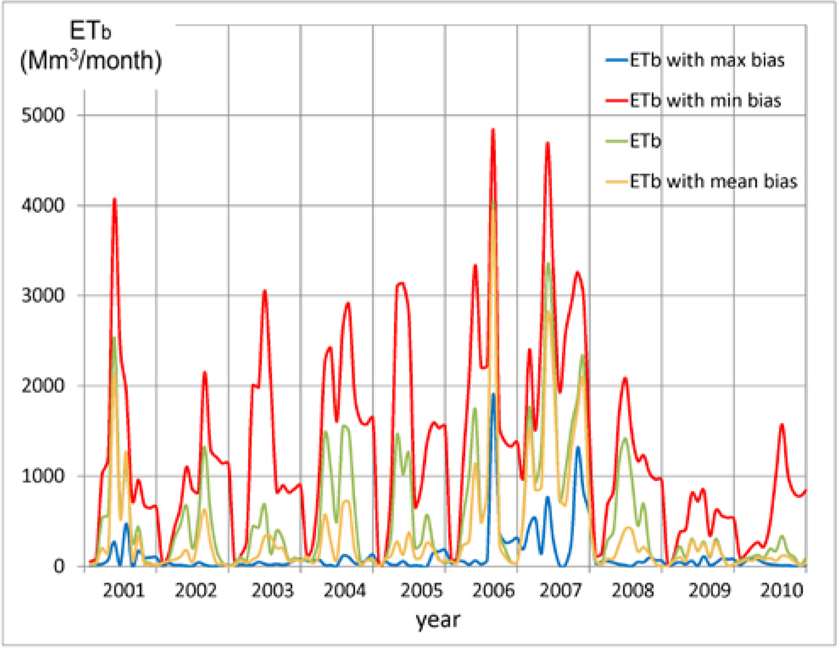
Since the principal aspect of the ETb method used is the definition of the bias curves, this section analyzes whether the ETb estimates are sensitive to the bias assignment. Figure 5 shows the monthly ETb results obtained in the province of Sichuan in the irrigated pixels as indicated in Figure 1. Four cases were considered depending on the bias assigned per month: (i) maximum of all classes; (ii) minimum of all classes; (iii) bias assigned based on the classification and (iv) mean bias calculated in all rain-fed croplands when no classes are considered.
All four cases show maximum values of ETb in the years 2006 and 2007. However, inter-annual variability was found to be sensitive to the selection of the bias. ETb presented low monthly values in most of the study period when using the maximum bias, whereas higher values and relatively regular patterns were obtained with the minimum bias. The curves obtained with the mean and assigned-per-class bias showed intermediate values, with ETb in general lower in the former case. In this context, Romaguera et al. [22] showed that the bias estimation was improved when using different classes instead of a single mean bias obtained for all rain-fed pixels. Therefore, despite the possible ETb similarities between these two cases, the classification approach is preferred to evaluate ETb.
5. Discussion
This paper illustrates preliminary results of the potential of using a remote sensing based method for obtaining time series of blue water evapotranspiration and combining it with the source of irrigation to monitor irrigation practices. The details and drawbacks of the models and data used were discussed in Romaguera et al. [21,22] and Thenkabail et al. [30].
The outputs produced in this paper need to be understood as preliminary examples of application. A better understanding of the ETactual inputs used would be required in order to obtain concluding outcomes. Regarding the bias, Section 4.3 showed how the ETb estimates were sensitive to the bias assignment.
Accuracies, Errors and Uncertainties
The uncertainties in ETactual estimation from remote sensing and the land surface modelling played an important role in the total ETb uncertainty. Kalma et al. [53] showed that remote sensing data provided typically relative errors of 15%–30% in ETactual estimation. In the case of the GLDAS products, the ETactual accuracy was not sufficiently evaluated in the literature, although some estimates exist. Fang et al. [54] reported the uncertainty in GLDAS–ET estimates by continent as equivalent heights of water based on 1979–2007 outputs from the four models included in the system. The climatology values of ETactual were 550 mm/year in Africa and 430 mm/year in Asia, with an uncertainty of ±60 mm/year in both cases. Besides, the definition of the bias curves has a standard deviation associated to the spatial averaging of the values per class. Despite the lack of detailed information about the GLDAS–ET accuracies, the aforementioned quantities were used (not shown here) to obtain the contributions of these three aspects to the total uncertainty by using the first order Taylor series expansion, where the covariance terms were neglected (inputs are independent) and linearity was assumed. A typical daily ETactual rate of 5 mm, a 30% in error of RS–ET, an average uncertainty of 5 mm/month in GLDAS–ET, and a bias curve in the Sichuan province were assumed. It was found that the error in RS–ET was the major contributor (50%–95%), modulated by the error of the bias which oscillated in time from around 5%–50%. The contribution of the GLDAS–ET inaccuracy was negligible. Increasing daily ETactual rates resulted in higher relative contribution of RS–ET, as expected, while decreasing the role of the bias, and being insignificant, the GLDAS–ET impact. Decreasing daily ETactual rates resulted in higher relative contribution of GLDAS–ET, with a maximum of 20% when a low value of daily ETactual was considered (0.1 mm/day).
These values served as an indication of the relative importance of RS–ET, GLDAS–ET and the bias, to the total uncertainty of ETb. In the case of irrigated areas, ETactual values are expected to be high, and therefore the role of the bias accuracy is less significant. However a better estimate of the GLDAS–ET uncertainty is required to properly quantify the different contributions.
Moreover, the accuracy of the static GlobCover and GIAM maps may decrease in time. These are used in the method to define rain-fed areas and to assign the type of irrigation respectively. Therefore, they are also a source of uncertainty.
The results in this paper were aggregated per country/province, which may be appropriate for regional planning purposes. However, specific spatial features may be lost in big areas due to the aggregation process, such as multiple cropping practices. Therefore, analysis at different spatial scales is recommended when examining particular features. Besides, the spatial resolution of the input data may be a limitation in heterogeneous areas, and therefore scaling techniques [55,56] are advised for understanding the sub-pixel variability.
In order to obtain concluding results about the application shown in this paper, long time series of data are desired to be able to properly analyze trends, and possible anomalies in the climatology. From the point of view of the land surface models, global data can be obtained for long time periods, from the year 1970 until the present for the Noah model in GLDAS. However, remote sensing ETactual outputs are more limited in time and space and depend a lot on the geometry of observation, technical characteristics, and lifetime of the sensors on board the satellites. In this context, Mu et al. [57] provided global ETactual products every eight days at 1 km resolution between the years 2001–2010. Their algorithm is based on the Penman-Monteith equation using daily meteorological reanalysis data and 8-day remotely sensed vegetation property dynamics from the Moderate–Resolution Imaging Spectroradiometer (MODIS) as inputs.
In general terms, the interpretation of the results regarding irrigation practices bears an uncertainty related to the multiple situations that can be found in reality. Water availability and decisions taken by the farmers to irrigate or not and how much, are factors that influence the results. However, in the face of an extreme event like a drought, the results obtained in the case studies of the present paper indicated the possibility of identifying and explaining the episode in terms of irrigated water.
Finally, compared with the existing literature about ETb given by Liu and Yang [16] and Mekonnen and Hoekstra [19], the method applied in this paper is innovative in two aspects: first it uses physically based remote sensing data instead of statistical data, and second it provides a better temporal resolution, more suitable for water management applications. Moreover, from an implementation point of view the method has a reasonably straightforward application procedure.
6. Conclusions
This paper illustrates the potential of using remote sensing and simulated actual evapotranspiration (ETactual) time series combined with an existing “type of irrigation” map, to monitor irrigation practice. It provides new tools to obtain monthly blue evapotranspiration (ETb) and shows the application in two relevant study areas: the Horn of Africa and the Chinese province of Sichuan, both affected by a drought event during the periods of analysis, but with differences in terms of water control and storage infrastructure. Further, monthly ETb are subdivided into the source of irrigation water: surface water, groundwater and conjunctive use, which relates to the availability of water resources.
The preliminary results show seasonal and inter-annual patterns in ETb. In the face of an extreme event like a drought, changes in ETb (i.e., irrigated water) can be identified, as well as the relative use of different sources of irrigation water. In Ethiopia, total ETb is estimated to decrease from 21 Mm3/month in the wet year 2010 to 10 Mm3/month in the dry year 2011, while ETb from groundwater increased; in Sichuan ETb is estimated at 200 Mm3/month in the wet year 2005 and 400 Mm3/month in the dry year 2006; these very different patterns of drought response, as found for the two locations, are qualitatively consistent with the literature. However, further research is needed to fully understand the whole of the temporal patterns found.
The research also reveals methodological and data limitations. The results in Sichuan are found to be dependent on the bias assignment required in the method. Moreover, particular spatial ETactual patterns are encountered in the input data. Finally, the use of longer time series of data for better interpretation of the results is recommended.
The application shown in this paper is innovative compared to similar literature in two aspects: first it uses physically based remote sensing data instead of statistical data, and second it provides a better temporal resolution, more suitable for water management applications. This paper constitutes a starting point for global temporal ETb analysis, applying an innovative remote sensing based approach and further research will contribute to the achievement of more concluding and operative results. In the field of water management, the approach has potential to assess the existence of irrigation, the source of irrigation water, the duration and variability in time, at pixel and country scales, and could be especially useful to monitor irrigation practice during periods of drought.
Acknowledgments
The authors wish to thank the Land Surface Analysis Satellite Applications Facility (LSA–SAF) of the European Organisation for the Exploitation of Meteorological Satellites (EUMETSAT), as well as the European Space Agency (ESA) and the ESA GlobCover Project, led by MEDIAS–France, for providing the products used in this paper. The GLDAS data used in this study were acquired as part of the mission of NASA’s Earth Science Division and archived and distributed by the Goddard Earth Sciences (GES) Data and Information Services Center (DISC). The authors also wish to thank the SPOT/VEGETATION data center ( www.vgt.vito.be) for the NDVI imagery and Prasad Thenkabail for providing the Global Irrigated Area Map.
Author Contributions
This work was carried out in the framework of the PhD research of the first author M. Romaguera. The coauthors are the supervisors linked to this project.
Conflicts of Interest
The authors declare no conflict of interest.
References
- FAO: Aquastat Database—Food and Agriculture Organization of the United Nations. Rome, Italy. Available online: http://faostat.Fao.Org/site/544/default.Aspx (accessed on 1 June 2014).
- Postel, S.L.; Daily, G.C.; Ehrlich, P.R. Human appropriation of renewable fresh water. Science 1996, 271, 785–788. [Google Scholar]
- Seckler, D.; Amarasinghe, U.; Molden, D.J.; de Silva, R.; Barker, R. World Water Demand and Supply, 1990–2025: Scenarios and Issues; IWMI: Colombo, Sri Lanka, 1998. [Google Scholar]
- Rockstrom, J.; Gordon, L.; Falkenmark, M.; Folke, C.; Engvall, M. Linkages among water vapor flows, food production, and terrestrial ecosystem services. Conserv. Ecol 1999, 3, 5. [Google Scholar]
- Shiklomanov, I.A.; Rodda, J.C. World Water Resources at the Beginning of the Twenty-First Century; Cambridge University Press: Cambridge, UK, 2003. [Google Scholar]
- Hoekstra, A.Y.; Hung, P.Q. A Quantification of Virtual Water Flows between Nations in Relation to International Crop Trade; UNESCO–IHE: Delft, The Netherlands, 2002. [Google Scholar]
- Chapagain, A.K.; Hoekstra, A.Y. Water Footprints of Nations; UNESCO–IHE: Delft, The Netherlands, 2004. [Google Scholar]
- Hoekstra, A.Y.; Chapagain, A.K. Water footprints of nations: Water use by people as a function of their consumption pattern. Water Resour. Manag 2007, 21, 35–48. [Google Scholar]
- Hoekstra, A.Y.; Chapagain, A.K. Globalization of Water. Sharing the Planet’s Freshwater Resources; Blackwell Publishing: Oxford, UK, 2008; pp. 1–208. [Google Scholar]
- Alcamo, J.; Florke, M.; Marker, M. Future long-term changes in global water resources driven by socio-economic and climatic changes. Hydrol. Sci. J. J. Sci. Hydrol 2007, 52, 247–275. [Google Scholar]
- Döll, P.; Siebert, S. Global modeling of irrigation water requirements. Water Resour. Res 2002, 38. [Google Scholar] [CrossRef]
- Rost, S.; Gerten, D.; Bondeau, A.; Lucht, W.; Rohwer, J.; Schaphoff, S. Agricultural green and blue water consumption and its influence on the global water system. Water Resour. Res 2008, 44. [Google Scholar] [CrossRef]
- Siebert, S.; Döll, P. The Global Crop Water Model (GCWM): Documentation and First Results for Irrigated Crops; Institute of Physical Geography, University of Frankfurt (Main): Frankfurt, Germany, 2008. [Google Scholar]
- Siebert, S.; Döll, P. Quantifying blue and green virtual water contents in global crop production as well as potential production losses without irrigation. J. Hydrol 2010, 384, 198–217. [Google Scholar]
- Liu, J.G.; Zehnder, A.J.B.; Yang, H. Global consumptive water use for crop production: The importance of green water and virtual water. Water Resour. Res 2009, 45. [Google Scholar] [CrossRef]
- Liu, J.G.; Yang, H. Spatially explicit assessment of global consumptive water uses in cropland: Green and blue water. J. Hydrol 2010, 384, 187–197. [Google Scholar]
- Hanasaki, N.; Inuzuka, T.; Kanae, S.; Oki, T. An estimation of global virtual water flow and sources of water withdrawal for major crops and livestock products using a global hydrological model. J. Hydrol 2010, 384, 232–244. [Google Scholar]
- Fader, M.; Gerten, D.; Thammer, M.; Heinke, J.; Lotze-Campen, H.; Lucht, W.; Cramer, W. Internal and external green-blue agricultural water footprints of nations, and related water and land savings through trade. Hydrol. Earth Syst. Sci 2011, 15, 1641–1660. [Google Scholar]
- Mekonnen, M.M.; Hoekstra, A.Y. The green, blue and grey water footprint of crops and derived crop products. Hydrol. Earth Syst. Sci 2011, 15, 1577–1600. [Google Scholar]
- Pfister, S.; Bayer, P.; Koehler, A.; Hellweg, S. Environmental impacts of water use in global crop production: Hotspots and trade-offs with land use. Environ. Sci. Technol 2011, 45, 5761–5768. [Google Scholar]
- Romaguera, M.; Krol, M.S.; Salama, M.S.; Hoekstra, A.Y.; Su, Z. Determining irrigated areas and quantifying blue water use in Europe using remote sensing Meteosat Second Generation (MSG) products and Global Land Data Assimilation System (GLDAS) data. Photogramm. Eng. Remote Sens 2012, 78, 861–873. [Google Scholar]
- Romaguera, M.; Salama, S.; Krol, M.S.; Hoekstra, A.Y.; Su, Z. Towards the improvement of blue evapotranspiration estimates by combining remote sensing and model simulation. Remote Sens 2014, 6, 7026–7049. [Google Scholar]
- Bastiaanssen, W.G.M.; Bos, M.G. Irrigation performance indicators based on remotely sensed data: A review of literature. Irrig. Drain. Syst 1999, 13, 192–311. [Google Scholar]
- Santos, C.; Lorite, I.J.; Tasumi, M.; Allen, R.G.; Fereres, E. Performance assessment of an irrigation scheme using indicators determined with remote sensing techniques. Irrig. Sci 2010, 28, 461–477. [Google Scholar]
- D'Urso, G.; De Michele, C.; Vuolo, F. Operational irrigation services from remote sensing: The irrigation advisory plan for the campania region, Italy. In Remote Sensing and Hydrology; Neale, C.M.U., Cosh, M.H., Eds.; Int. Assoc. Hydrological Sciences: Wallingford, WA, USA, 2012; Volume 352, pp. 419–422. [Google Scholar]
- Siebert, S.; Döll, P.; Hoogeveen, J.; Faures, J.M.; Frenken, K.; Feick, S. Development and validation of the global map of irrigation areas. Hydrol. Earth Syst. Sci 2005, 9, 535–547. [Google Scholar]
- Siebert, S.; Hoogeveen, J.; Frenken, K. Irrigation in Africa, Europe and Latin America. Update of the Digital Global Map of Irrigation Areas to Version 4; Institute of Physical Geography, University of Frankfurt (Main): Frankfurt, Germany, 2006. [Google Scholar]
- Ozdogan, M.; Gutman, G. A new methodology to map irrigated areas using multi-temporal MODIS and ancillary data: An application example in the continental US. Remote Sens. Environ 2008, 112, 3520–3537. [Google Scholar]
- Thenkabail, P.S.; Biradar, C.M.; Noojipady, P.; Dheeravath, V.; Li, Y.J.; Velpuri, M.; Gumma, M.; Gangalakunta, O.R.P.; Turral, H.; Cai, X.L.; et al. Global irrigated area map (GIAM), derived from remote sensing, for the end of the last millennium. Int. J. Remote Sens 2009, 30, 3679–3733. [Google Scholar]
- Thenkabail, P.S.; Biradar, C.M.; Noojipady, P.; Dheeravath, V.; Li, Y.J.; Velpuri, M.; Reddy, G.P.O.; Cai, X.L.; Gumma, M.; Turral, H.; et al. A Global Irrigated Area Map (GIAM) Using Remote Sensing at the End of the Last Millenium; International Water Management Institute: Colombo, Sri Lanka, 2008; p. 63. [Google Scholar]
- Ozdogan, M.; Rodell, M.; Beaudoing, H.K.; Toll, D.L. Simulating the effects of irrigation over the united states in a land surface model based on satellite-derived agricultural data. J. Hydrometeorol 2010, 11, 171–184. [Google Scholar]
- UCLouvain; ESA. Globcover 2009. Products Description and Validation Report; European Space Agency: Paris, France, 2011. [Google Scholar]
- LSA–SAF. LSA–SAF Validation Report. Products LSA–16 (MET), LSA–17 (DMETt); Doc. Num. SAF/LAND/RMI/VR/0.6; The EUMETSAT Network of Satellite Application Facilities: Darmstadt, Germany, 2010. [Google Scholar]
- Rezaee, M.R.; Lelieveldt, B.P.F.; Reiber, J.H.C. A new cluster validity index for the fuzzy c-mean. Pattern Recognit. Lett 1998, 19, 237–246. [Google Scholar]
- Ghilain, N.; Arboleda, A.; Gellens-Meulenberghs, F. Evapotranspiration modelling at large scale using near-real time MSG SEVIRI derived data. Hydrol. Earth Syst. Sci 2011, 15, 771–786. [Google Scholar]
- Chen, X. The Plateau Scale Land—Air Interaction and Its Connections to Troposphere and Lower Stratosphere. PhD Thesis, ITC Dissertation 237, Faculty of Geo-Information and Earth Observation (ITC). University of Twente, Enschede, The Netherlands, 2013. [Google Scholar]
- Chen, X.; Su, Z.; Ma, Y.; Liu, S.; Xu, Z. Development of a 10 year (2001–2010) 0.1° dataset of land-surface energy balance for mainland China. Atmos. Chem. Phys. Discuss 2014, 14, 14471–14518. [Google Scholar]
- Gellens-Meulenberghs, F.; Arboleda, A.; Ghilain, N. Towards a continuous monitoring of evapotranspiration based on MSG data. Proceedings of IAHS Symposium on Remote Sensing for Environmental Monitoring and Change Detection, Perugia, Italy, 2–13 July 2007; IAHS Press: Wallingford, WA, USA.
- Su, Z. The surface energy balance system (SEBS) for estimation of turbulent heat fluxes. Hydrol. Earth Syst. Sci 2002, 6, 85–99. [Google Scholar]
- Chen, F.; Mitchell, K.; Schaake, J.; Xue, Y.K.; Pan, H.L.; Koren, V.; Duan, Q.Y.; Ek, M.; Betts, A. Modeling of land surface evaporation by four schemes and comparison with FIFE observations. J. Geophys. Res. Atmos 1996, 101, 7251–7268. [Google Scholar]
- Rodell, M.; Houser, P.R.; Jambor, U.; Gottschalck, J.; Mitchell, K.; Meng, C.J.; Arsenault, K.; Cosgrove, B.; Radakovich, J.; Bosilovich, M.; et al. The Global Land Data Assimilation System. Bull. Am. Meteorol. Soc 2004, 85, 381–394. [Google Scholar]
- Anderson, W.B.; Zaitchik, B.F.; Hain, C.R.; Anderson, M.C.; Yilmaz, M.T.; Mecikalski, J.; Schultz, L. Towards an integrated soil moisture drought monitor for East Africa. Hydrol. Earth Syst. Sci 2012, 16, 2893–2913. [Google Scholar]
- Viste, E.; Korecha, D.; Sorteberg, A. Recent drought and precipitation tendencies in Ethiopia. Theor. Appl. Climatol 2013, 112, 535–551. [Google Scholar]
- Awulachew, S.B.; Yilma, A.D.; Loulseged, M.; Loiskandl, W.; Ayana, M.; Alamirew, T. Water Resources and Irrigation Development in Ethiopia. IWMI Working Paper 123; International Water Management Institute (IWMI): Colombo, Sri Lanka, 2007; p. 66. [Google Scholar]
- Onimus, F. Ethiopia—Irrigation and Drainage Project: P092353—Implementation Status Results Report: Sequence 15; World Bank: Washington, DC, USA, 2014. [Google Scholar]
- Zhang, S.H.; Yi, Y.J.; Liu, Y.; Wang, X.K. Hydraulic principles of the 2268-year-old Dujiangyan project in China. J. Hydraul. Eng. ASCE 2013, 139, 538–546. [Google Scholar]
- Dai, Z.J.; Du, J.Z.; Li, J.F.; Li, W.H.; Chen, J.Y. Runoff characteristics of the Changjiang river during 2006: Effect of extreme drought and the impounding of the Three Gorges dam. Geophys. Res. Lett 2008, 35. [Google Scholar] [CrossRef]
- Wang, Y.Q.; Shi, J.C.; Liu, Z.H.; Liu, W.J. Application of Microwave Vegetation Index (MVI) to monitoring drought in Sichuan Province of China. Proceedings of 2012 First International Conference on Agro-Geoinformatics (Agro-Geoinformatics), Shanghai, China, 2–4 August 2012; pp. 458–463.
- Hendrix, M. Water in Ethiopia: Drought, disease and death. Glob. Major. E J 2012, 3, 110–120. [Google Scholar]
- FAOSTAT. Food and Agriculture Organization of the United Nations, FAOSTAT Database. Available online: http://faostat3.Fao.Org/faostat-gateway/go/to/download/q/qc/e (accessed on 27 April 2014).
- See, L.; McCallum, I.; Fritz, S.; Perger, C.; Kraxner, F.; Obersteiner, M.; Baruah, U.D.; Mili, N.; Kalita, N.R. Mapping cropland in Ethiopia using crowdsourcing. Int. J. Geosci 2013, 4, 6–13. [Google Scholar]
- National Data Base. National Bureau of Statistics of China. Available online: http://data.Stats.Gov.Cn/index (accessed on 17 April 2014).
- Kalma, J.D.; McVicar, T.R.; McCabe, M.F. Estimating land surface evaporation: A review of methods using remotely sensed surface temperature data. Surv. Geophys 2008, 29, 421–469. [Google Scholar]
- Fang, H.; Beaudoing, H.K.; Rodell, M.; Teng, W.L.; Vollmer, B.E. Global Land Data Assimilation System (GLDAS) products, services and applications from NASA Hydrology Data and Information Services Center (HDISC). Proceedings of the ASPRS 2009 Annual Conference, Baltimore, Maryland, 8–13 March 2009.
- Anderson, M.C.; Kustas, W.P.; Norman, J.M. Upscaling flux observations from local to continental scales using thermal remote sensing. Agron. J 2007, 99, 240–254. [Google Scholar]
- Jia, S.; Zhu, W.; Lű, A.; Yan, T. A statistical spatial downscaling algorithm of TRMM precipitation based on NDVI and DEM in the Qaidam basin of China. Remote Sens. Environ 2011, 115, 3069–3079. [Google Scholar]
- Mu, Q.Z.; Zhao, M.S.; Running, S.W. Improvements to a MODIS global terrestrial evapotranspiration algorithm. Remote Sens. Environ 2011, 115, 1781–1800. [Google Scholar]


| Data | Source | Spatial Coverage | Spatial Resolution | Temporal Resolution | Details |
|---|---|---|---|---|---|
| ETactual | LSA–SAF * | MSG disk ** | 3 km at nadir | daily | Availability of data: Europe: Jan. 2007–present The rest: Sept. 2009–present Used for the study area in Africa |
| Chen et al. [36,37] (SEBS model) | China | 0.1° | monthly | Availability of data: Years 2001–2010 Used for the study area in China | |
| GLDAS (Noah model) | Global | 0.25° (∼30 km at equator) | monthly | Availability of data: March 2000–present | |
| Land Cover | MERIS | Global | 300 m | Static | GlobCover map calculated in year 2009 |
| Rn, P | GLDAS (Noah model) | Global | 0.25° (∼30 km at equator) | monthly | Availability of data: February 2000–present |
| NDVI | AVHRR | Africa | 1 km | monthly | Generated by IGBP Period: April 1992–March 1993 Used for the study area in Africa |
| SPOT–VEG | Global | 1 km | monthly | Used for the study area in China | |
| Irrigation source | GIAM | Global | 10 km | Static | Data: Type of irrigation Primary data used: —AVHRR from 1997–1999 —TOA NDVI from 1982–2000 |
*List of acronyms: LSA–SAF (Land Surface Analysis–Satellite Applications Facility); MSG (Meteosat Second Generation); GLDAS (Global Land Data Assimilation System); SEBS (Surface Energy Balance System); MERIS (Medium Resolution Imaging Spectrometer); Rn (Net Radiation); P (Precipitation); Normalized Difference Vegetation Index (NDVI); AVHRR (Advanced Very High Resolution Radiometer); IGBP (International Geosphere–Biosphere Programme Data); SPOT–VEG (Satellite Pour l’Observation de la Terre–Vegetation); GIAM (Global Irrigated Area Map); TOA (Top Of Atmosphere);**Meteosat disk covers latitudes between −60° and +60° and longitudes between −60° to +60°.
© 2014 by the authors; licensee MDPI, Basel, Switzerland This article is an open access article distributed under the terms and conditions of the Creative Commons Attribution license (http://creativecommons.org/licenses/by/4.0/).
Share and Cite
Romaguera, M.; Krol, M.S.; Salama, M.S.; Su, Z.; Hoekstra, A.Y. Application of a Remote Sensing Method for Estimating Monthly Blue Water Evapotranspiration in Irrigated Agriculture. Remote Sens. 2014, 6, 10033-10050. https://doi.org/10.3390/rs61010033
Romaguera M, Krol MS, Salama MS, Su Z, Hoekstra AY. Application of a Remote Sensing Method for Estimating Monthly Blue Water Evapotranspiration in Irrigated Agriculture. Remote Sensing. 2014; 6(10):10033-10050. https://doi.org/10.3390/rs61010033
Chicago/Turabian StyleRomaguera, Mireia, Maarten S. Krol, Mhd. Suhyb Salama, Zhongbo Su, and Arjen Y. Hoekstra. 2014. "Application of a Remote Sensing Method for Estimating Monthly Blue Water Evapotranspiration in Irrigated Agriculture" Remote Sensing 6, no. 10: 10033-10050. https://doi.org/10.3390/rs61010033