Comparison of Classification Algorithms and Training Sample Sizes in Urban Land Classification with Landsat Thematic Mapper Imagery


Abstract
:
1. Introduction
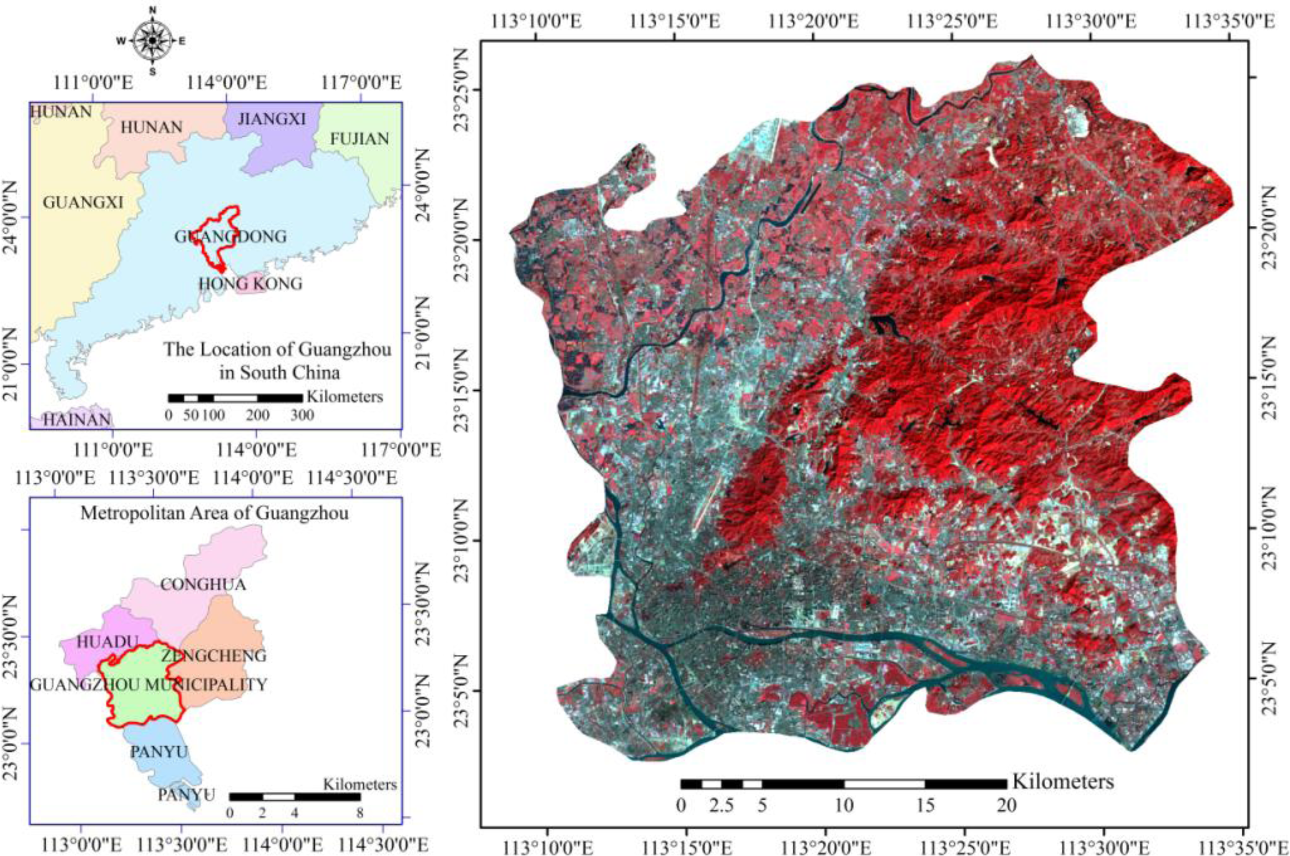
2. Study Site and Data
3. Method
3.1. Classification System
3.2. Training Samples
3.3. Test Samples
3.4. Classification Process
3.5. Active Learning
4. Results
4.1. Pixel-Based Classification
4.2. Objected-Oriented Classification
5. Discussions
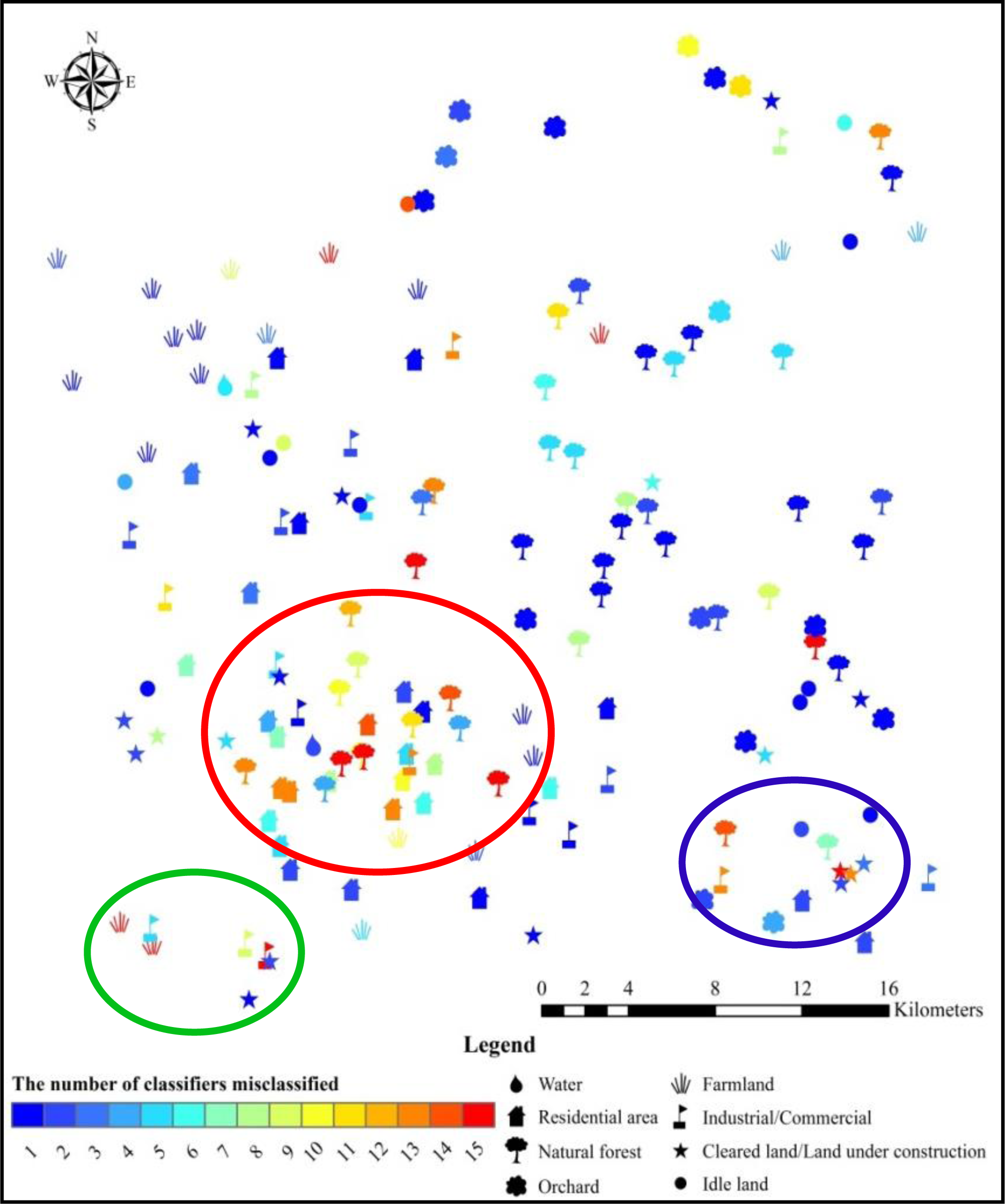
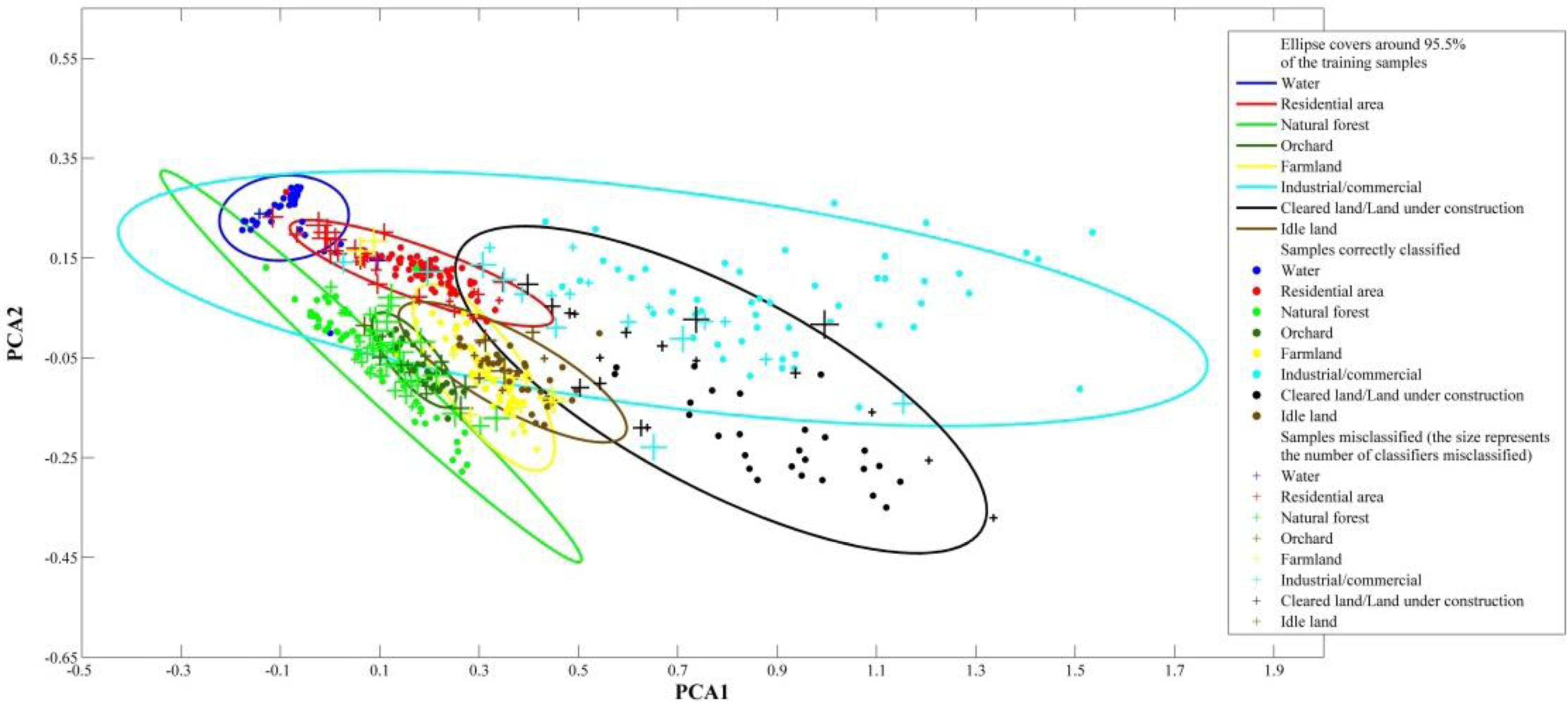
5.1. Most Common Errors among the Classifiers
5.2. The Comparison of the Algorithms Using Pixel-Based Method
5.3. The Impact of Different Training Set Sizes
5.4. Algorithm Performances with Low-Quality Training Samples
6. Summary
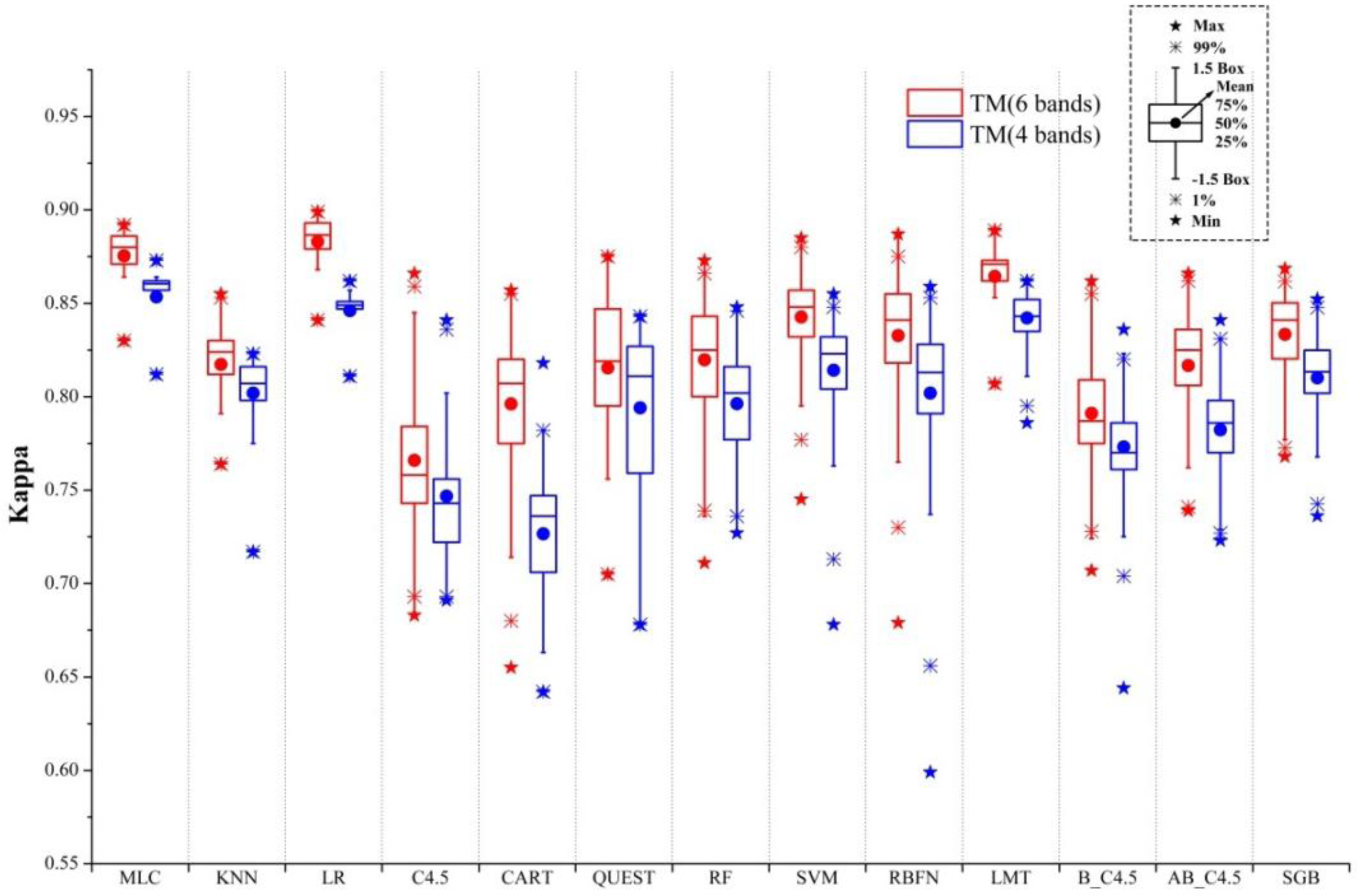
- (1)
- The 4-band set of TM data by excluding the two middle infrared bands resulted in Kappa accuracies in the range between 0.818 and 0.873. The inclusion of the two middle infrared bands in the 6-band case increased this range to 0.850 and 0.899. This indicates the potential loss of overall accuracies in urban and rural urban fringe environments with the lack of middle infrared bands could be within 3%–5%.
- (2)
- Unsupervised algorithms could produce as good classification results as some of the supervised ones when a sufficient number of clusters are produced and clusters can be identified by an image analyst who is familiar with the study area. The accuracy of the unsupervised algorithms produced better than 0.841 Kappa accuracies for the eight land cover and land use classes.
- (3)
- Most supervised algorithms could produce high classification accuracies if the parameters are properly set and training samples are sufficiently representative. In this condition, MLC, LR, and LMT algorithms are more proper for users. These algorithms can be easily used with relatively more stable performances.
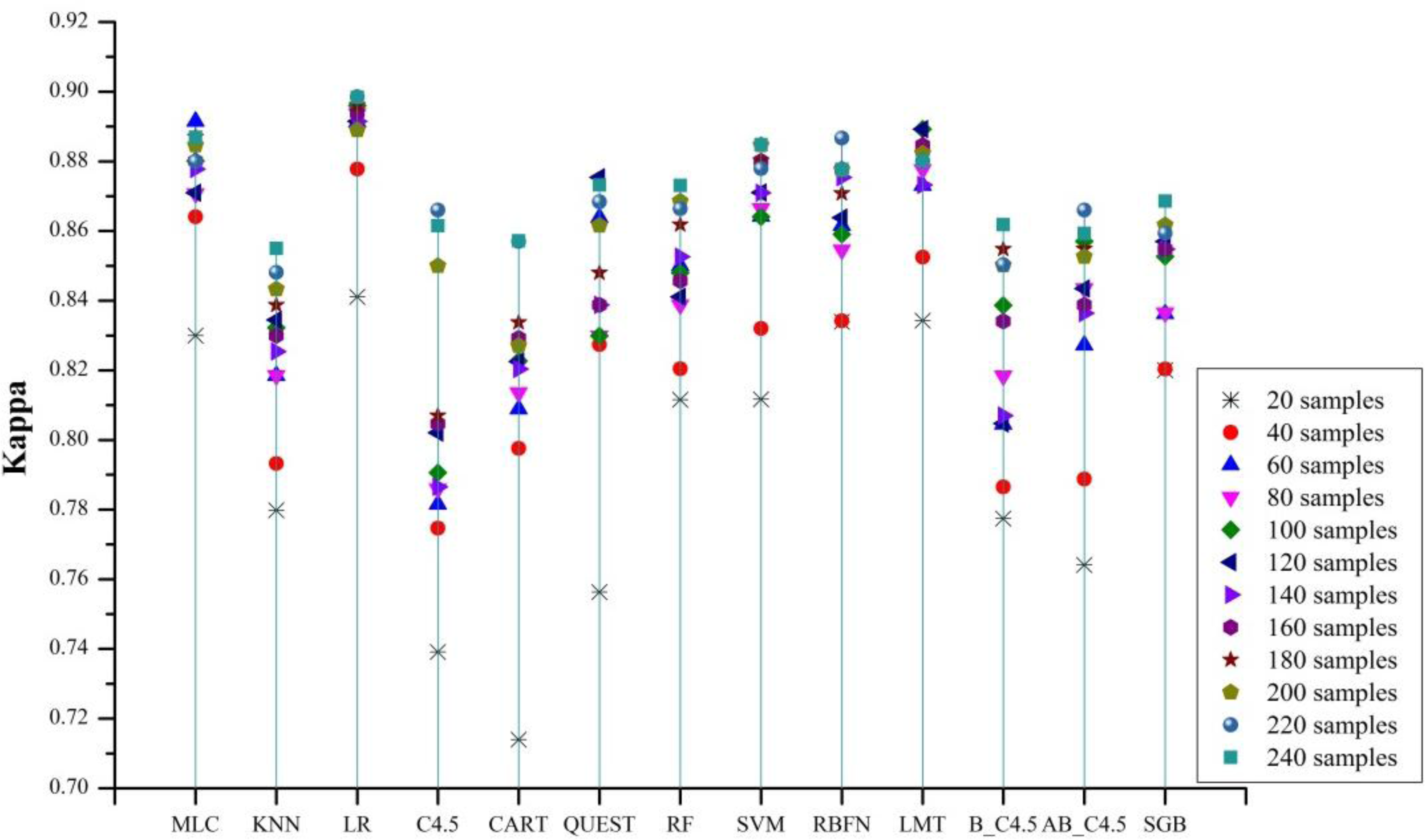
- (4)
- Insufficient (less representative) training caused large accuracy drops (0.06–0.15) in all supervised algorithms. Among all the algorithms tested, MLC, LR, SVM, and LMT are the least affected by the size of training sets. When using a small-sized training set, MLC, LR, SVM, RBFN, and LMT performed well.
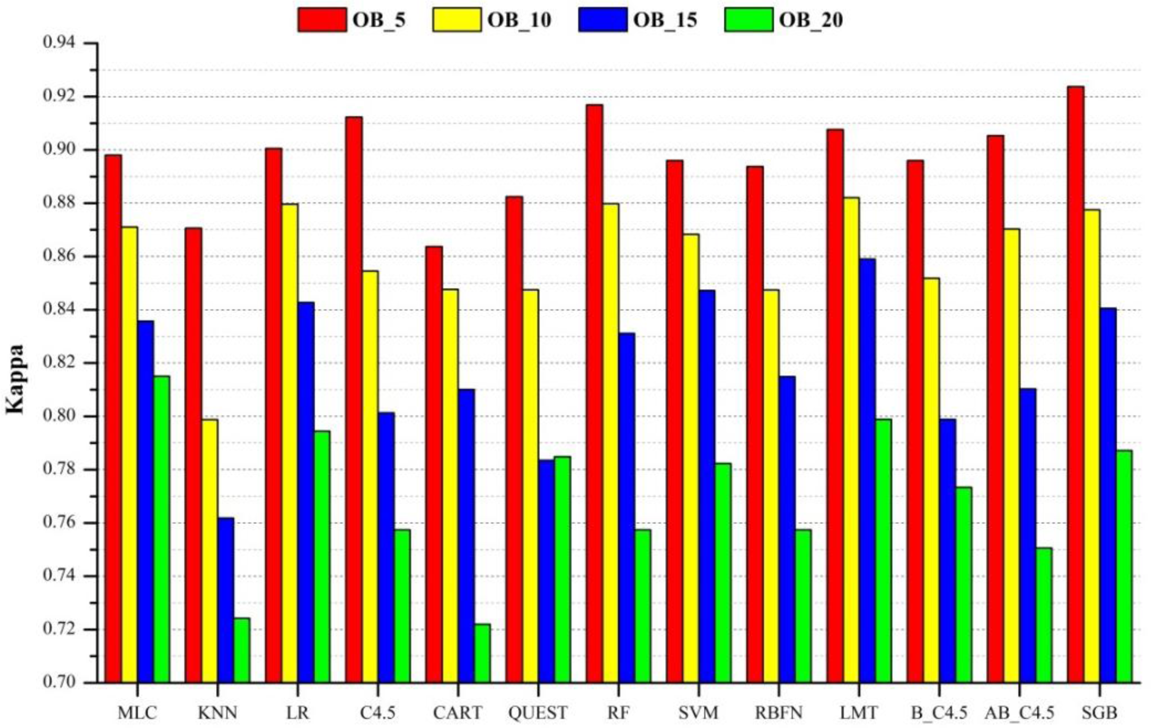
- (5)
- In segment-based classification experiments, most algorithms performed better when the segment size was the smallest (with a scale factor of 5). At the scale of 5, SGB outperformed all other algorithms by producing the highest Kappa values of 0.924 and this is followed by RF. All algorithms are less sensitive to the large increase of data dimensionality. MLC, LR, RF, SVM, LMT, and SGB algorithms are the best choices to do the classification. They could produce relatively good accuracy at different scales.
Acknowledgments
Author Contributions
Conflicts of Interest
References
- Lu, D.S.; Weng, Q.H. A survey of image classification methods and techniques for improving classification performance. Int. J. Remote Sens 2007, 28, 823–870. [Google Scholar]
- Gong, P.; Howarth, P.J. Land-use classification of SPOT HRV data using a cover-frequency method. Int. J. Remote Sens 1992, 13, 1459–1471. [Google Scholar]
- Pu, R.L.; Landry, S.; Yu, Q. Object-based detailed land-cover classification with high spatial resolution IKONOS imagery. Int. J. Remote Sens 2011, 32, 3285–3308. [Google Scholar]
- Shackelford, A.K.; Davis, C.H. A hierarchical fuzzy classification approach for high resolution multispectral data over urban areas. IEEE Trans. Geosci. Remote Sens 2003, 41, 1920–1932. [Google Scholar]
- Tzeng, Y.C.; Fan, K.T.; Chen, K.S. An adaptive thresholding multiple classifiers system for remote sensing image classification. Photogramm. Eng. Remote Sens 2009, 75, 679–687. [Google Scholar]
- Wilkinson, G.G. Results and implications of a study of fifteen years of satellite image classification experiments. IEEE Trans. Geosci. Remote Sens 2005, 43, 433–440. [Google Scholar]
- Gong, P.; Howarth, P.J. An assessment of some factors influencing multispectral land-cover classification. Photogramm. Eng. Remote Sens 1990, 56, 597–603. [Google Scholar]
- Fan, F.L.; Wang, Y.P.; Qiu, M.H.; Wang, Z.S. Evaluating the temporal and spatial urban expansion patterns of Guangzhou from 1979 to 2003 by remote sensing and GIS methods. Int. J. Geogr. Inf. Sci 2009, 23, 1371–1388. [Google Scholar]
- Fan, F.L.; Weng, Q.H.; Wang, Y.P. Land use and land cover change in Guangzhou, China, from 1998 to 2003, based on Landsat TM/ETM+ imagery. Sensors 2007, 7, 1223–1342. [Google Scholar]
- Seto, K.; Woodcock, C.; Song, C.H.; Huang, X.; Lu, J.; Kaufmann, R.K. Monitoring land-use change in the Pearl River Delta using Landsat TM. Int. J. Remote Sens 2002, 23, 1985–2004. [Google Scholar]
- Song, C.; Woodcock, C.E.; Seto, K.C.; Lenney, M.P; Macomber, S.A. Classification and change detection using Landsat TM data: When and how to correct atmospheric effects? Remote Sens. Environ 2001, 75, 230–244. [Google Scholar]
- Gong, P.; Marceau, D.; Howarth, P.J. A comparison of spatial feature extraction algorithms for land-use mapping with SPOT HRV data. Remote Sens. Environ 1992, 40, 137–151. [Google Scholar]
- Gong, P.; Wang, J.; Yu, L.; Zhao, Y.; Zhao, Y.; Liang, L.; Niu, Z.; Huang, X.; Fu, H.; Liu, S.; et al. Finer resolution observation and monitoring of global land cover: First mapping results with landsat TM and ETM+ data. Int. J. Remote Sens 2013, 34, 2607–2654. [Google Scholar]
- Foody, G.M.; Mathur, A.; Sanchez-Hernandez, C.; Boyd, D.S. Training set size requirements for the classification of a specific class. Remote Sens. Environ 2006, 104, 1–14. [Google Scholar]
- Mather, P.M. Computer Processing of Remotely-Sensed Images, 3rd ed; John Wiley & Sons, Ltd: Chichester, UK, 2004. [Google Scholar]
- Piper, J. Variability and bias in experimentally measured classifier error rates. Pattern Recognit. Lett 1992, 13, 685–692. [Google Scholar]
- Van Niel, T.; McVicar, T.; Datt, B. On the relationship between training sample size and data dimensionality: Monte Carlo analysis of broadband multi-temporal classification. Remote Sens. Environ 2005, 98, 468–480. [Google Scholar]
- Congalton, R.G.; Green, K. Assessing the Accuracy of Remotely Sensed Data: Principles and Practices; CRC Press: Boca Raton, FL, USA, 1999; p. 137. [Google Scholar]
- Ball, G.H.; Hall, D.J. Isodata, a Novel Method of Data Analysis and Pattern Classification; Stanford Research Institute: Menlo Park, CA, USA, 1965. [Google Scholar]
- Chen, Y.; Gong, P. Clustering based on eigenspace transformation—CBEST for efficient classification. ISPRS J. Photogramm. Remote Sens 2013, 83, 64–80. [Google Scholar]
- Aha, D.W.; Kibler, D.; Albert, M.K. Instance-based learning algorithms. Mach. Learn 1991, 6, 37–66. [Google Scholar]
- Le Cessie, S.; van Houwelingen, J.C. Ridge estimators in logistic regression. Appl. Stat 1992, 41, 191–201. [Google Scholar]
- Quinlan, R. C4.5: Programs for Machine Learning; Morgan Kaufmann Publishers: San Mateo, CA, USA, 1993. [Google Scholar]
- Breiman, L.; Friedman, J.H.; Olshen, R.A.; Stone, C.J. Classification and Regression Trees; Wadsworth Press: Monterey, CA, USA, 1984. [Google Scholar]
- Loh, W.Y.; Shih, Y.S. Split selection methods for classification trees. Stat. Sin 1997, 7, 815–840. [Google Scholar]
- Breiman, L. Random forests. Mach. Learn 2001, 45, 5–32. [Google Scholar]
- Chang, C.C.; Lin, C.J. LIBSVM: A library for support vector machines. ACM Trans. Intell. Syst. Technol 2011, 2, 1–27. [Google Scholar]
- Bishop, C.M. Neural Networks for Pattern Recognition; Oxford University Press: New York, NY, USA, 1995. [Google Scholar]
- Niels, L.; Mark, H.; Eibe, F. Logistic model trees. Mach. Learn 2005, 95, 161–205. [Google Scholar]
- Sumner, M.; Frank, E.; Hall, M.A. Speeding up Logistic Model Tree Induction. Proceedings of the 9th European Conference on Principles and Practice of Knowledge Discovery in Databases, Porto, Portugal, 3–7 October 2005; pp. 675–683.
- Breiman, L. Bagging predictors. Mach. Learn 1996, 24, 123–140. [Google Scholar]
- Freund, Y.; Robert, E. Schapire: Experiments with a New Boosting Algorithm. Proceedings of the 13th International Conference on Machine Learning, Bari, Italy, 3–6 July 1996.
- Friedman, J.H. Stochastic gradient boosting. Comput. Stat. Data Anal 2002, 38, 367–378. [Google Scholar]
- Bradski, G. The OpenCV library. Dr. Dobb’s J. Softw. Tools 2000, 25, 120–125. [Google Scholar]
- Witten, I.H.; Frank, E. Data Mining, Practical Machine Learning Tools and Techniques, 2nd ed; Morgan Kaufmann Publishers: San Francisco, CA, USA, 2005; p. 525. [Google Scholar]
- Hall, M.; Frank, E.; Holmes, G.; Pfahringer, B.; Reutemann, P.; Witten, I.H. The WEKA data mining software: An update. SIGKDD Explor 2009, 11, 10–18. [Google Scholar]
- Ridgeway, G. Generalized Boosted Models: A Guide to the GBM Package. Available online: https://r-forge.r-roject.org/scm/viewvc.php/*checkout*/pkg/inst/doc/gbm.pdf?revision=17&root=gbm&pathrev=18 (accessed on 21 September 2009).
- Clinton, N.; Holt, A.; Scarborough, J.; Yan, L.; Gong, P. Accuracy assessment measures for object based image segmentation goodness. Photogramm. Eng. Remote Sens 2010, 76, 289–299. [Google Scholar]
- Clinton, N. BerkeleyImageSeg User’s Guide. CiteSeerX 2010. Available online: http://citeseerx.ist.psu.edu/viewdoc/download?doi=10.1.1.173.1324&rep=rep1&type=pdf (accessed on 16 January 2014). [Google Scholar]
- Tuia, D.; Volpi, M.; Copa, L.; Kanevski, M.; Munoz-Mari, J. A survey of active learning algorithms for supervised remote sensing image classification. IEEE J. Sel. Top. Signal Process 2011, 5, 606–616. [Google Scholar]
- Campbell, C.; Cristianini, N.; Smola, A.J. Query Learning with Large Margin Classifiers. In the Proceedings of the 17th International Conference on Machine Learning, Stanford, CA, USA, 29 June–2 July 2000.
- Schohn, G.; Cohn, D. Less is More: Active Learning with Support Vector Machines. Proceedings of the 17th International Conference on Machine Learning, 29 June–2 July 2000; San Francisco, CA, USA.
- Strobl, C.; Malley, J.; Tutz, G. Supplement to “An Introduction to Recursive Partitioning: Rational, Application, and Characteristics of Classification and Regression Trees, Bagging, and Random Forests”. Available online: http://supp.apa.org/psycarticles/supplemental/met_14_4_323/met_14_4_323_supp.html (accessed on 11 November 2010).
- Wang, L.; Sousa, W.; Gong, P. Integration of object-based and pixel-based classification for mangrove mapping with IKONOS imagery. Int. J. Remote Sens 2004, 25, 5655–5668. [Google Scholar]
- Gong, P.; Howarth, P.J. The use of structural information for improving land-cover classification accuracies at the rural-urban fringe. Photogramm. Eng. Remote Sens 1990, 56, 67–73. [Google Scholar]
- Gong, P.; Howarth, P.J. Frequency-based contextual classification and grey-level vector reduction for land-use identification. Photogramm. Eng. Remote Sens 1992, 58, 423–437. [Google Scholar]
- Xu, B.; Gong, P.; Seto, E.; Spear, R. Comparison of different gray-level reduction schemes for a revised texture spectrum method for land-use classification using IKONOS imagery. Photogramm. Eng. Remote Sens 2003, 6, 529–536. [Google Scholar]
- Liu, D.; Kelly, M.; Gong, P. A spatial-temporal approach to monitoring forest disease spread using multi-temporal high spatial resolution imagery. Remote Sens. Environ 2006, 101, 167–180. [Google Scholar]
- Cai, S.S.; Liu, D.S. A comparison of object-based and contextual pixel-based classifications using high and medium spatial resolution images. Remote Sens. Lett 2013, 4, 998–1007. [Google Scholar]
- Wolf, N. Object features for pixel-based classification of urban areas comparing different machine learning algorithms. Photogramm. Fernerkund 2013, 3, 149–161. [Google Scholar]
- Luo, L.; Mountrakis, G. Converting local spectral and spatial information from a priori classifiers into contextual knowledge for impervious surface classification. ISPRS J. Photogramm. Remote Sens 2011, 66, 579–587. [Google Scholar]
- Weng, Q.H. Remote sensing of impervious surfaces in the urban areas: Requirements, methods, and trends. Remote Sens. Environ 2012, 117, 34–49. [Google Scholar]
- Gamba, P. Human settlements: A global challenge for EO data processing and interpretation. IEEE Proc 2013, 101, 570–581. [Google Scholar]
- Mountrakis, G.; Xi, B. Assessing reference dataset representativeness through confidence metrics based on information density. ISPRS J. Photogramm. Remote Sens 2011, 78, 129–147. [Google Scholar]


| Land-Use Types | Description |
|---|---|
| Water | Water bodies such as reservoirs, ponds and river |
| Residential area | Residential areas where driveways and roof tops dominate |
| Natural forest | Large area of trees |
| Orchard | Large area of fruit trees planted |
| Farmland | Fields where vegetables or crops grow |
| Industrial/commercial | Lands where roof tops of large buildings dominate |
| Cleared land/Land under construction | Lands where vegetation is denuded or where the construction is underway |
| Idle land | Lands where no vigorous vegetation grows |
| Algorithm | Abbreviation | Parameter Type | Parameter Set | Source of Codes |
|---|---|---|---|---|
| ISODATA | ISODATA | Number of Clusters Maximum Iterations | 100, 150 100 | ENVI |
| CBEST | CBEST | Number of Clusters Maximum Iterations | 100, 150 100 | CBEST |
| Maximum-likelihood classification | MLC | Mean and covariance matrix | Estimated from training samples | openCV |
| K-nearest neighbor | KNN | K weight | 1,3,5,7,9,11 No weighting, 1/distance | Weka |
| Logistic regression | LR | Ridge estimator | 0, 10−1, 10−2, 10−3, 10−4, 10−5, 10−6, 10−7, 10−8 | Weka |
| C4.5 | C4.5 | MinNumObj Confidence | 1, 2, 3, 4, 5, 6, 7, 8, 9, 10 0.05f, 0.1f, 0.2f, 0.3f, 0.4f, 0.5f | Weka |
| Classification and Regression Tree | CART | MinNumObj | 1, 2, 3, 4, 5, 6, 7, 8, 9, 10 | Weka |
| Quick, Unbiased, Efficient, and Statistical Tree algorithm | QUEST | Split types MinNumObj | univariate, linear 1, 2, 3, 4, 5, 6, 7, 8, 9, 10 | QUEST |
| Random Forests | RF | numFeature numTrees | For 6-bands: 1,2,3,4,5,6 For 4-bands: 1,2,3,4 20, 40, 60, 80, 100, 120, 140, 160, 180, 200 | Weka |
| Support Vector Machine | SVM | kernelType Cost gamma | radial basis function 10, 20, 30, 40, 50, 60, 70, 80, 90, 100 2−2, 2−1, 1, 21, 22, 23, 24, 25, 26, 27 | Libsvm |
| Radial Basis Function Network | RBFN | MaxIteration NumCluster minStdDev | 500, 1,000, 3,000, 5,000, 7,000 2, 3, 4, 5, 6, 7, 8, 9 0, 0.01, 0.05, 0.1 | Weka |
| Logistic model tree | LMT | minNumInstances weightTrimBeta splitOnResiduals | 5, 10, 15, 20, 25, 30 0, 0.01, 0.05, 0.1 False (C4.5 splitting criterion), True (LMT criterion) | Weka |
| Bagging C4.5 | B_C4.5 | bagSizePercent numIterations classifier | 20, 40, 60, 80, 100 10, 50, 100, 150, 200 C4.5 | Weka |
| AdaBoost C4.5 | AB_C4.5 | weightThreshold numIterations classifier | 40, 60, 80, 100 10, 20, 30, 40, 50, 60, 70 C4.5 | Weka |
| Stochastic gradient boosting | SGB | n.trees shrinkage bag.fraction | 500, 1000 0.05, 0.1 0.2, 0.3, 0.4, 0.5, 0.6, 0.7, 0.8, 0.9 | R |
| Feature |
|---|
| Maximum value of the segments for each spectral band (6 bands) |
| Mean or average values of the segments for each spectral band (6 bands) |
| Minimum values of the segments for each spectral band (6 bands) |
| The standard deviations of the pixels in the segments for each spectral band (6 bands) |
| Algorithm | Parameter Choice | Accuracy |
|---|---|---|
| ISODATA | 6-Band, Number of Clusters = 150 | 0.864 |
| 4-Band, Number of Clusters = 150 | 0.841 | |
| CBEST | 6-Band, Number of Clusters = 150 | 0.850 |
| 4-Band, Number of Clusters = 150 | 0.846 | |
| MLC | 6-Band, 60 training samples | 0.892 |
| 4-Band, 60 training samples | 0.873 | |
| KNN | 6-Band, 240 training samples, K = 3, weight = 1/distance | 0.855 |
| 4-Band, 240 training samples, K = 3, weight = 1/distance | 0.823 | |
| LR | 6-Band, 220 training samples, Ridge estimator = 10−8 | 0.899 |
| 4-Band, 200 training samples, Ridge estimator = 10−8 | 0.862 | |
| C4.5 | 6-Band, 220 training samples, MinNumObj = 7, confidence = 0.2f | 0.866 |
| 4-Band, 240 training samples, MinNumObj = 3, confidence = 0.5f | 0.841 | |
| CART | 6-Band, 240 training samples, MinNumObj = 1 | 0.857 |
| 4-Band, 220 training samples, MinNumObj = 2 | 0.818 | |
| QUEST | 6-Band, 100 training samples, split type = linear, MinNumObj = 8/9/10 | 0.875 |
| 4-Band, 180 training samples, split type = linear, MinNumObj = 1–10 | 0.843 | |
| RF | 6-Band, 240 training samples, numFeatures = 1, numTrees = 20 | 0.873 |
| 4-Band, 200 training samples, numFeatures = 1, numTrees = 60 | 0.848 | |
| SVM | 6-Band, 240 training samples, kernelType = radial basis function, C = 80, gamma = 23 | 0.885 |
| 4-Band, 240 training samples, kernelType = radial basis function, C = 50, gamma = 24 | 0.855 | |
| RBFN | 6-Band, 220 training samples, minStdDev = 0.01, NumCluster = 9, MaxIts = 1,000 | 0.887 |
| 4-Band, 240 training samples, minStdDev = 0.01, NumCluster = 8, MaxIts = 3,000/5,000 | 0.859 | |
| LMT | 6-Band, 160 training samples, weightTrimBeta = 0, splitOnResiduals = C4.5 splitting criterion, minNumInstances ≥ 5 | 0.885 |
| 4-Band, 200 training samples, weightTrimBeta = 0.1, splitOnResiduals = LMT splitting criterion, minNumInstances ≥ 5 | 0.862 | |
| B_C4.5 | 6-Band, 240 training samples, bagSizePercent = 80, numIterations = 100 C4.5parameter (MinNumObj = 2, confidence = 0.3f) | 0.862 |
| 4-Band, 240 training samples, bagSizePercent = 60, numIterations = 10 C4.5parameter (MinNumObj = 1, confidence = 0.2f) | 0.836 | |
| AB_C4.5 | 6-Band, 220 training samples, weightThreshold = 40, numIterations ≥ 10, C4.5parameter (MinNumObj = 7, confidence = 0.2f) | 0.866 |
| 4-Band, 240 training samples, weightThreshold = 40, numIterations ≥ 10, C4.5parameter (MinNumObj = 5, confidence = 0.3f) | 0.841 | |
| SGB | 6-Band, 240 training samples, bag.fraction = 0.2, shrinkage = 0.1, n.tree = 1,000 | 0.869 |
| 4-Band, 220 training samples, bag.fraction = 0.2, shrinkage = 0.1, n.tree = 1,000 | 0.852 |
| OB_5 | |
|---|---|
| MLC | 0.898 |
| KNN | 0.871 |
| LR | 0.901 |
| C4.5 | 0.912 |
| CART | 0.864 |
| QUEST | 0.882 |
| RF | 0.917 |
| SVM | 0.891 |
| RBFN | 0.894 |
| LMT | 0.908 |
| B_C4.5 | 0.896 |
| AB_C4.5 | 0.891 |
| SGB | 0.924 |
| Class | Water | Residential Area | Natural Forest | Orchard | Farmland | Industrial/ Commercial | Cleared Land/ Land under Construction | Idle Land |
|---|---|---|---|---|---|---|---|---|
| ISODATA | 1 | 4 | 16 | 7 | 10 | 6 | 14 | 1 |
| CBEST | 0 | 7 | 13 | 8 | 12 | 7 | 7 | 11 |
| MLC | 1 | 5 | 20 | 2 | 6 | 8 | 3 | 2 |
| LR | 0 | 7 | 20 | 0 | 5 | 7 | 4 | 1 |
| KNN | 0 | 11 | 30 | 2 | 6 | 8 | 5 | 2 |
| C4.5 | 2 | 10 | 15 | 4 | 8 | 11 | 5 | 3 |
| CART | 0 | 11 | 27 | 2 | 8 | 8 | 3 | 3 |
| QUEST | 0 | 14 | 18 | 4 | 5 | 7 | 4 | 2 |
| RF | 0 | 14 | 17 | 4 | 8 | 7 | 3 | 2 |
| SVM | 0 | 13 | 22 | 1 | 5 | 6 | 2 | 1 |
| RBFN | 0 | 10 | 12 | 3 | 7 | 8 | 3 | 6 |
| LMT | 0 | 8 | 21 | 1 | 4 | 9 | 5 | 2 |
| B_C4.5 | 1 | 11 | 26 | 2 | 8 | 7 | 3 | 2 |
| AB_C4.5 | 2 | 10 | 15 | 4 | 8 | 11 | 5 | 3 |
| SGB | 0 | 12 | 21 | 2 | 8 | 9 | 4 | 1 |
| Class | Ground Truth (pixels) | |||||||||
|---|---|---|---|---|---|---|---|---|---|---|
| Water | Residential Area | Natural Forest | Orchard | Farmland | Industrial/Commercial | Cleared Land/Land under Construction | Idle land | Total | ||
| Classification results | Water | 41 | 1 | 0 | 0 | 0 | 0 | 0 | 0 | 42 |
| Residential area | 0 | 84 | 0 | 0 | 2 | 2 | 0 | 0 | 88 | |
| Natural forest | 0 | 0 | 63 | 0 | 1 | 0 | 0 | 0 | 64 | |
| Orchard | 0 | 0 | 18 | 48 | 0 | 0 | 0 | 0 | 66 | |
| Farmland | 0 | 0 | 2 | 0 | 72 | 0 | 0 | 1 | 75 | |
| Industrial/commercial | 0 | 6 | 0 | 0 | 0 | 64 | 4 | 0 | 74 | |
| Cleared land/Land under construction | 0 | 0 | 0 | 0 | 0 | 4 | 40 | 0 | 44 | |
| Idle land | 0 | 0 | 0 | 0 | 2 | 1 | 0 | 44 | 47 | |
| Total | 41 | 91 | 83 | 48 | 77 | 71 | 44 | 45 | 500 | |
© 2014 by the authors; licensee MDPI, Basel, Switzerland This article is an open access article distributed under the terms and conditions of the Creative Commons Attribution license (http://creativecommons.org/licenses/by/3.0/).
Share and Cite
Li, C.; Wang, J.; Wang, L.; Hu, L.; Gong, P. Comparison of Classification Algorithms and Training Sample Sizes in Urban Land Classification with Landsat Thematic Mapper Imagery. Remote Sens. 2014, 6, 964-983. https://doi.org/10.3390/rs6020964
Li C, Wang J, Wang L, Hu L, Gong P. Comparison of Classification Algorithms and Training Sample Sizes in Urban Land Classification with Landsat Thematic Mapper Imagery. Remote Sensing. 2014; 6(2):964-983. https://doi.org/10.3390/rs6020964
Chicago/Turabian StyleLi, Congcong, Jie Wang, Lei Wang, Luanyun Hu, and Peng Gong. 2014. "Comparison of Classification Algorithms and Training Sample Sizes in Urban Land Classification with Landsat Thematic Mapper Imagery" Remote Sensing 6, no. 2: 964-983. https://doi.org/10.3390/rs6020964