
Evaluation of the Airborne CASI/TASI Ts-VI Space Method for Estimating Near-Surface Soil Moisture

 ,
,
Abstract
:
1. Introduction
2. Airborne Experiment and SM Measurements
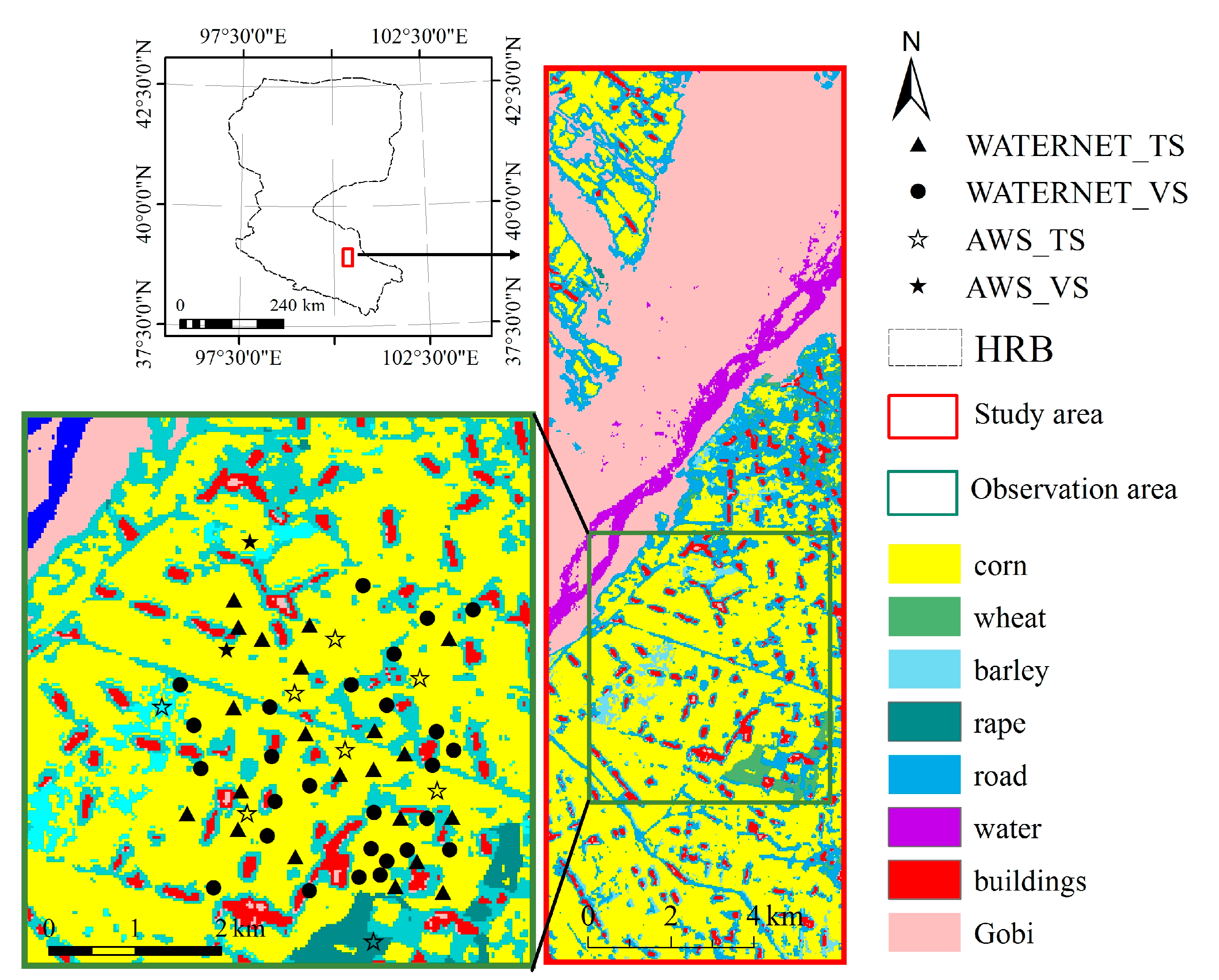
2.1. Study Area and Field Campaign

| WSN | Node Number | Fractional Vegetation Cover | Underlying Surface | ||
|---|---|---|---|---|---|
| Range | Mean | Standard Deviation | |||
| AWSs | 10 | 0.21–0.62 | 0.47 | 0.09 | cornfield |
| WATERNET | 48 | 0.38–0.68 | 0.51 | 0.06 | cornfield |

2.2. Airborne Hyperspectral Measurements
| Basic Specifications | CASI 1500 | TASI 600 |
|---|---|---|
| Spectral range | 380–1050 nm | 8–11.5 μm |
| Spectral resolution | 7.2 nm (48 bands) | 110 nm (32 bands) |
| Spectral width | 7 nm | 15 nm |
| Scan angle | 40° | 40° |
| Across-track pixels | 1500 | 600 |
| Spatial resolution | 1 m | 3 m |
3. Ts/VI Space Algorithm
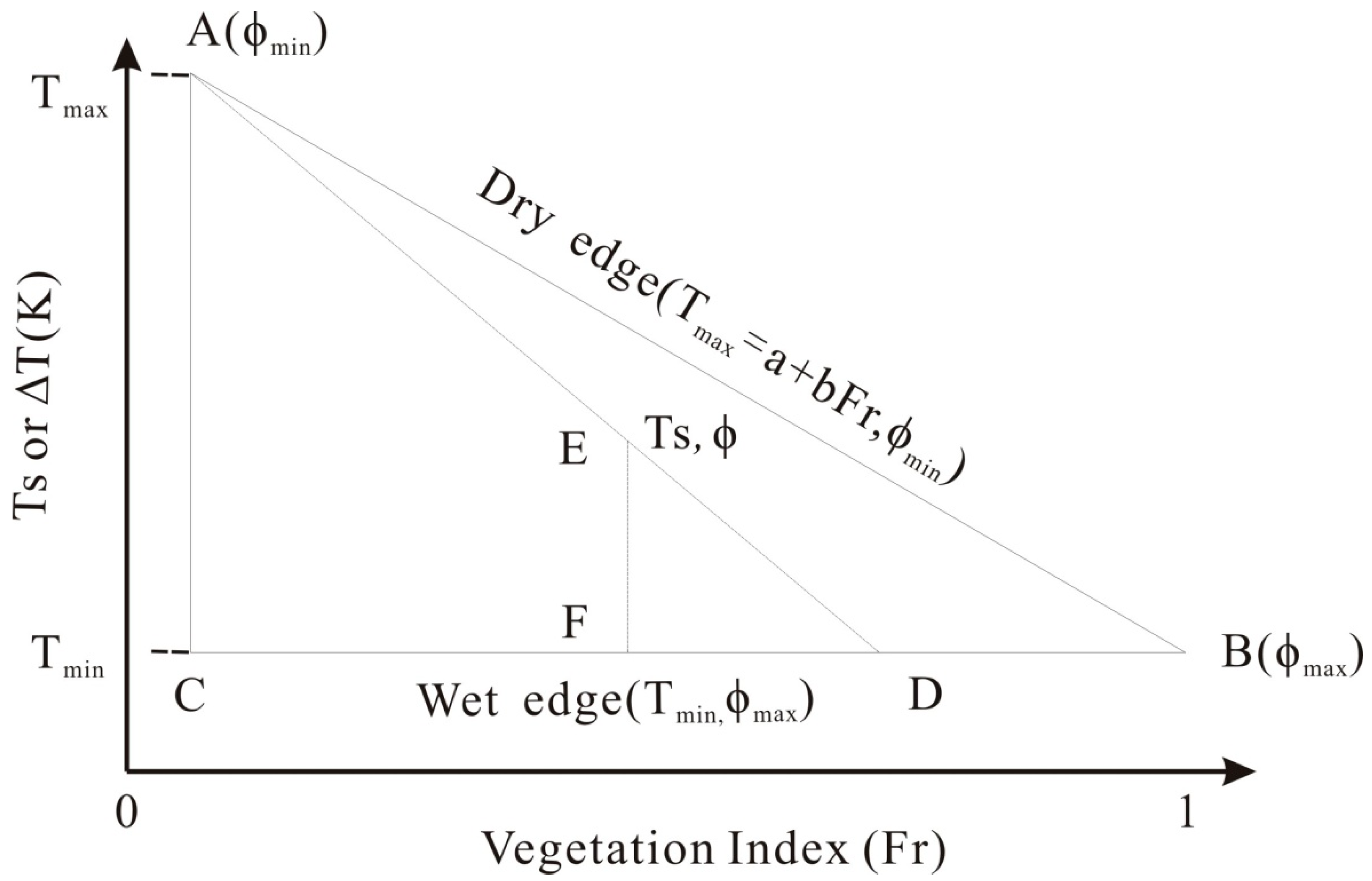
3.1. Theory of Ts/VI Space

3.2. SM Estimation from EF
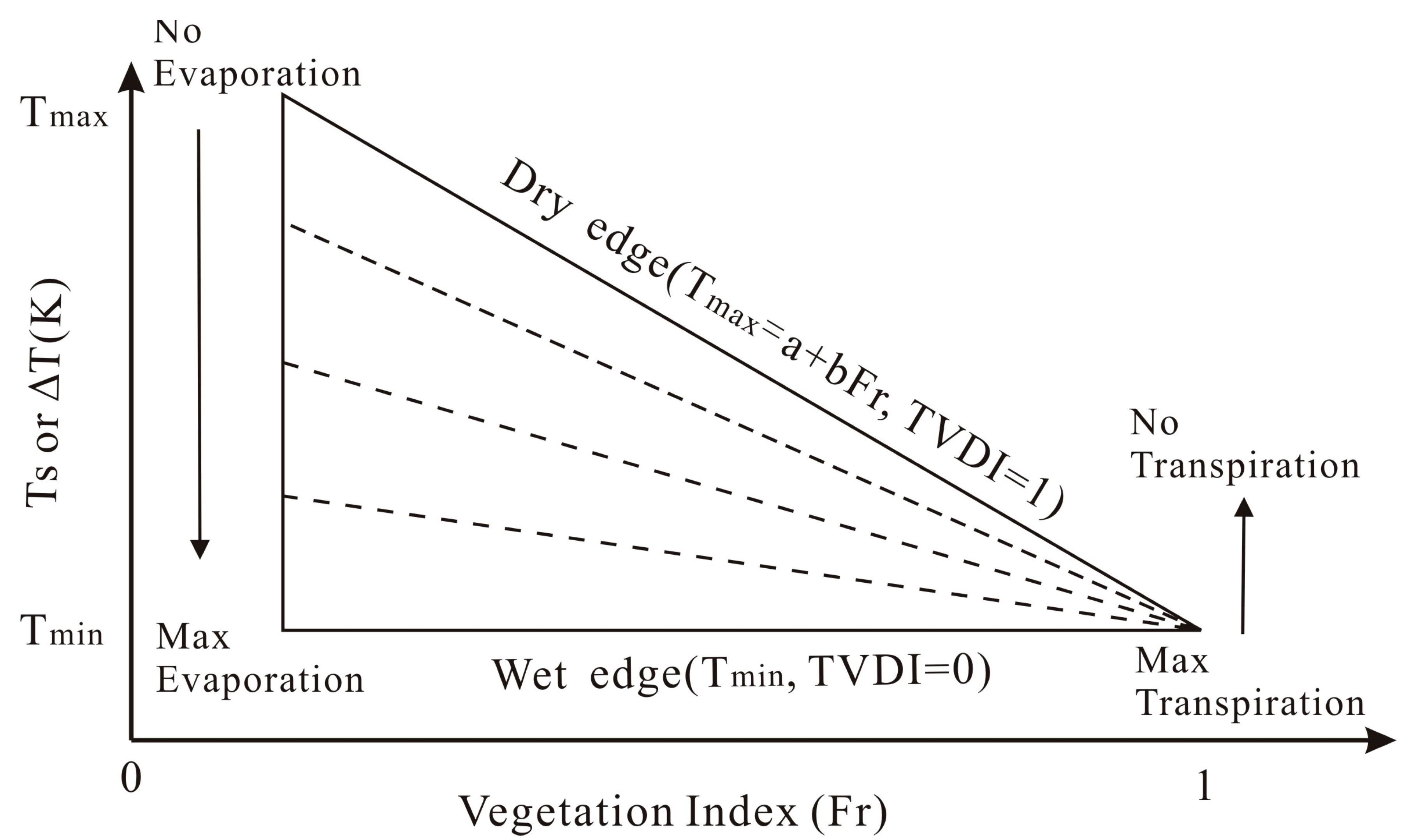
3.3. SM Estimations from the TVDI

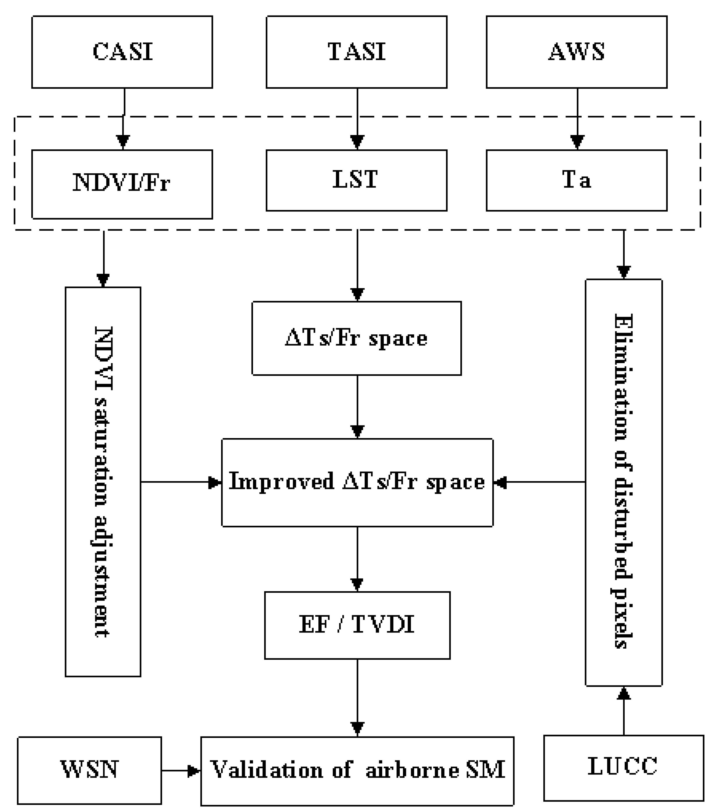
4. The Adaption of Airborne Ts/VI Space
4.1. De-saturated Space ( Space)


4.2. Non-Disturbed /Fr Space ( Space)
- (1)
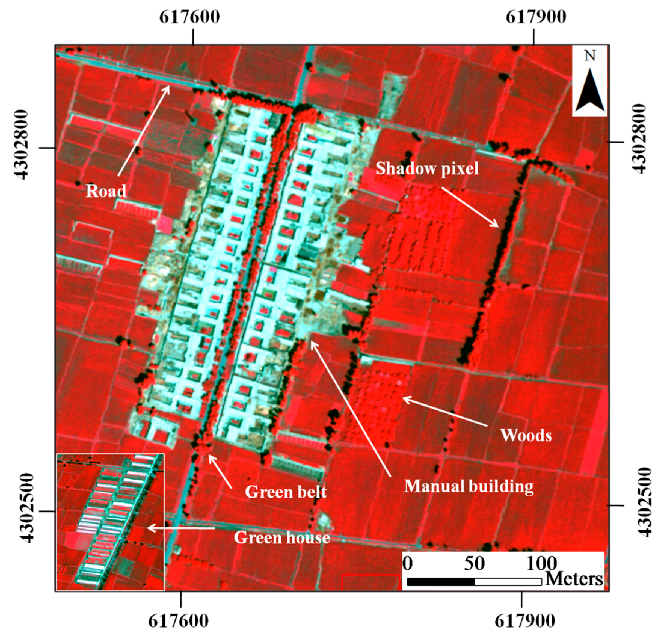
- Artificial facility pixels. The building and road pixels were recognized by LUCC data based on the same CASI data provided by HiWATER [54]. Many pathway pixels between farmlands were too shallow to display in LUCC data and were removed in step (4).
- (2)
- Shadowed pixels. The shadowed pixels were identified when their pixel reflectance values in the 554-nm CASI band were less than 0.027 [54].
- (3)
- Tree pixels. Woods were extracted when the areas were >20 m2 and when the reflectance variance in the CASI 554-nm band was >0.025. Green belts were identified when the ratio of the girth to the area was >0.38 and when the height was >15 m by using the vegetation height product with a spatial resolution of 1-m from the digital surface model [55].
- (4)
- Pathway, greenhouse, and outlier pixels. The common characteristics of these pixels were that they were all distributed in farmland. The pixels’ were much greater than the neighboring farmland pixels, and their NDVI values were much lower. Based on these characteristics, belt transect pixels covering areas of 1 km × 1 km were used to calculate the variance of (), and the NDVI variance () of each pixel. Combined with ground surveys and visual interpretations, the pixels with values less than 0.15 or values greater than 20 K2 were defined as disturbed pixels. Then, the pathway, greenhouse, and outlier pixels were removed from the study region using a 1 km × 1 km window size and thresholds of and .

5. Results
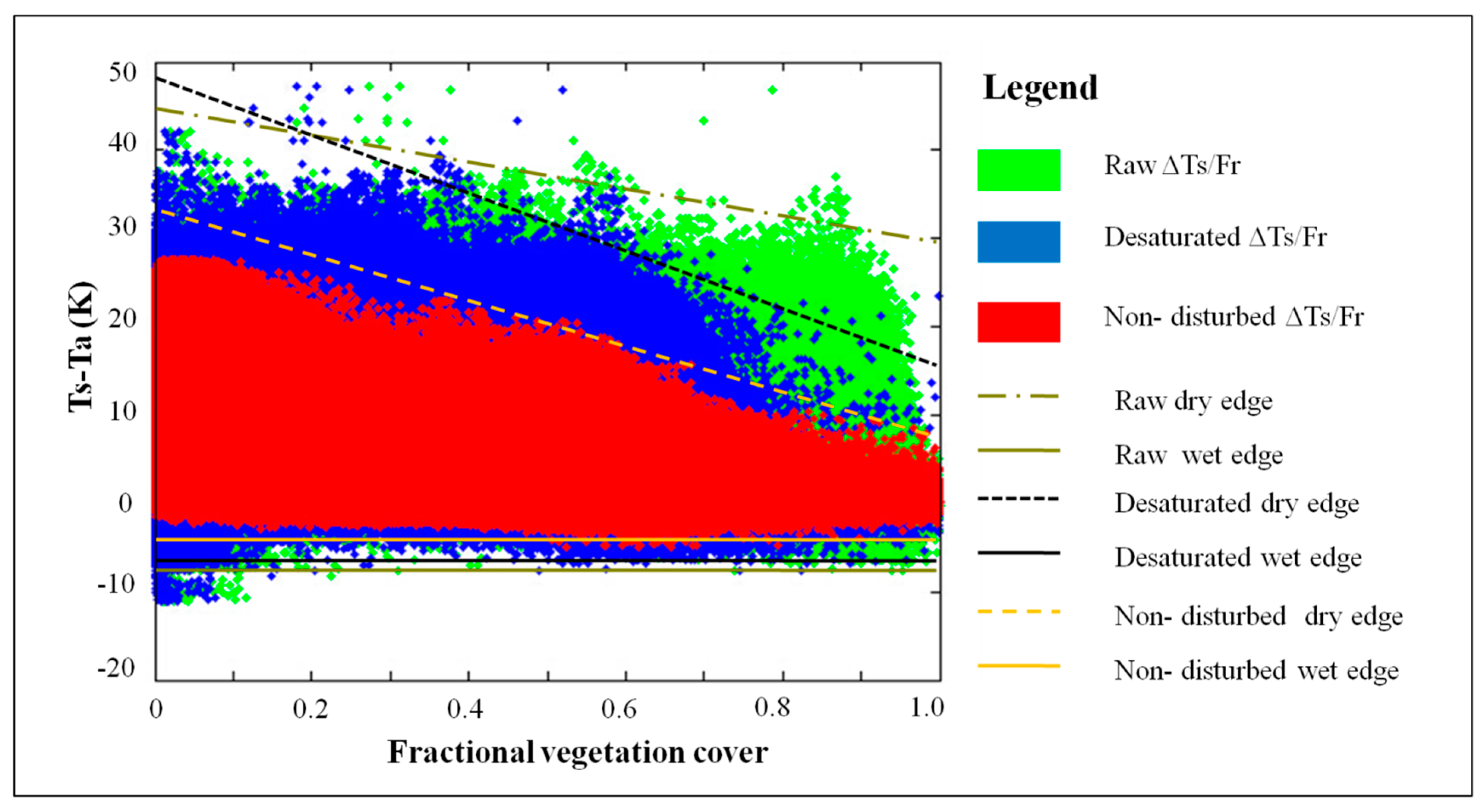
5.1. Analysis of /Fr Space
| /Fr | Dry/Wet Edge | Fitting Equation | r2 |
|---|---|---|---|
| Raw /Fr | Dry edge | y = −14.7x + 44 | 0.38 |
| Wet edge | y = 1.587x − 7 | 0.25 | |
| space | Dry edge | y = −30x + 47.1 | 0.78 |
| Wet edge | y = 0.72x − 7.5 | 0.31 | |
| space | Dry edge | y = −23.05x + 32 | 0.96 |
| Wet edge | y = −0.16x − 3 | 0.57 |
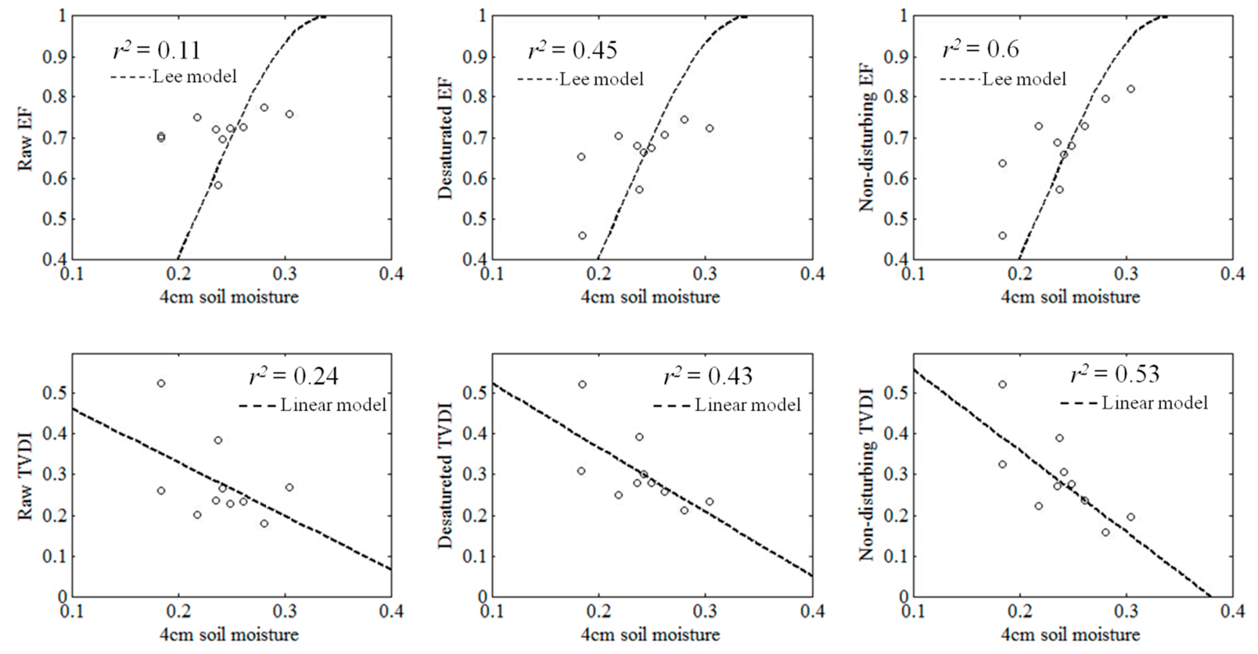
5.2. The Relationships between Dryness Indices and SM Contents at Different Depths
| SM Depth | ||||||
|---|---|---|---|---|---|---|
| r2 | r2 | r2 | r2 | r2 | r2 | |
| SM at a depth of 2 cm | 0.38 | 0.39 | 0.3 | 0.32 | 0.2 | 0.21 |
| SM at a depth of 4 cm | 0.6 | 0.53 | 0.45 | 0.43 | 0.11 | 0.24 |
| SM at a depth of 10 cm | 0.14 | 0.19 | 0.15 | 0.14 | null | 0.17 |
| SM at a depth of 20 cm | 0.13 | 0.12 | null | 0.12 | null | null |
| SM at a depth of 40 cm | null | null | null | null | null | null |
| SM at a depth of 60 cm | null | null | null | null | null | null |
| SM at a depth of 100 cm | null | null | null | null | null | null |

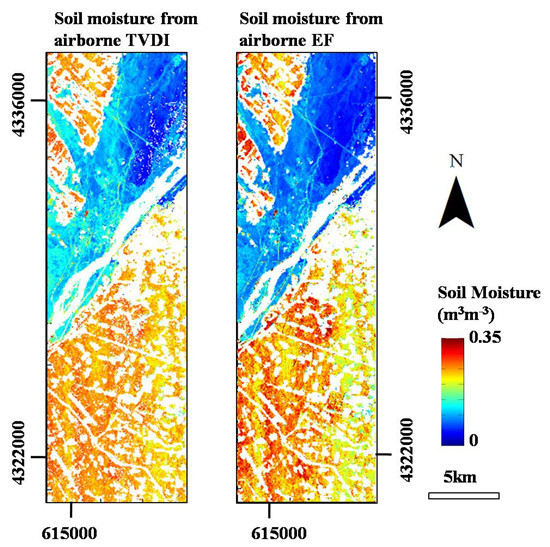
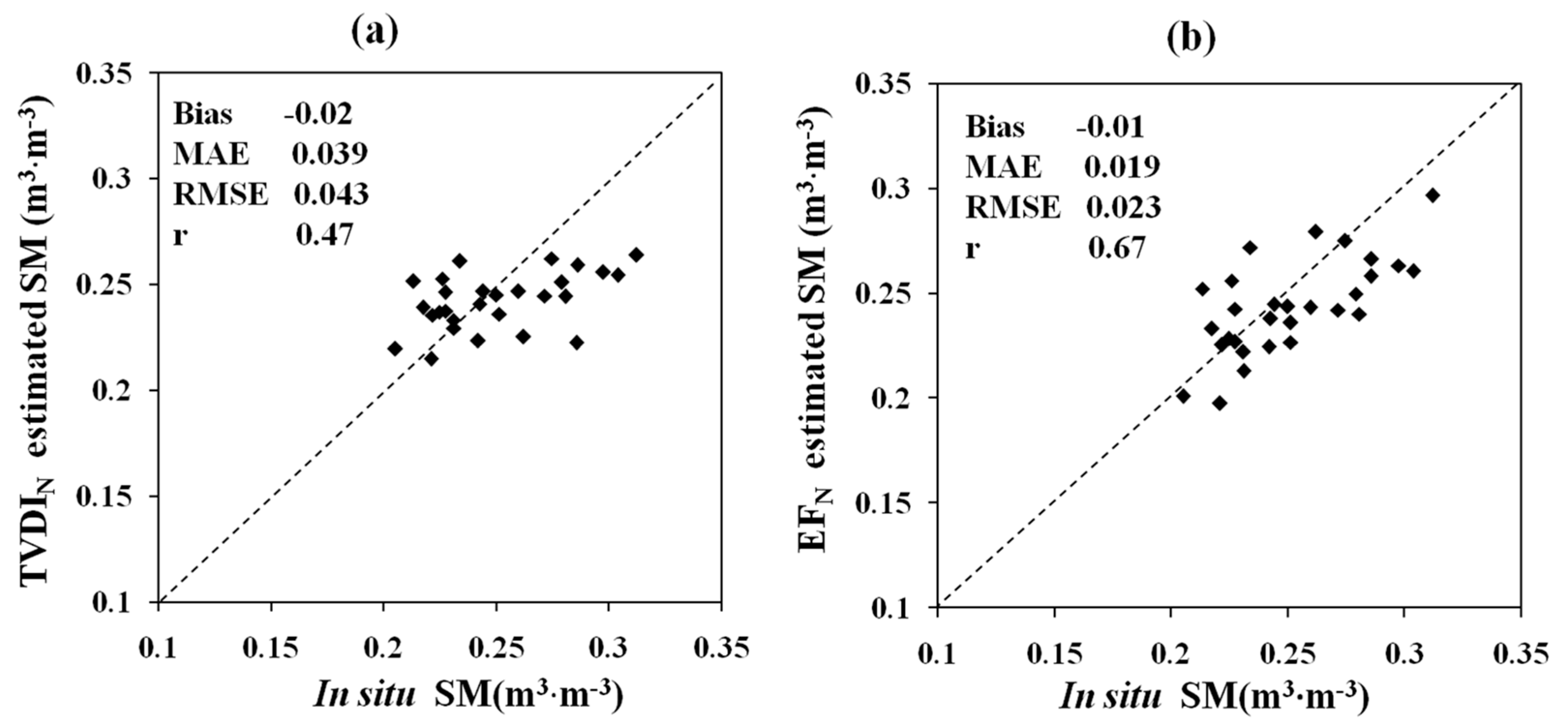
5.3. Validation and Evaluation of the Estimated SM


| Soil Moisture (m3·m−3) | Study Area | Validation Area | ||||
|---|---|---|---|---|---|---|
| Range | Mean | Standard Deviation | Range | Mean | Standard Deviation | |
| 0.01–0.336 | 0.188 | 0.075 | 0.15–0.336 | 0.251 | 0.021 | |
| 0.002–0.35 | 0.171 | 0.092 | 0.15–0.35 | 0.260 | 0.040 | |

6. Discussion
7. Conclusions
Acknowledgments
Author Contributions
Conflicts of Interest
References
- Gao, S.; Zhu, Z.; Liu, S.; Jin, R.; Yang, G.; Tan, L. Estimating the spatial distribution of soil moisture based on Bayesian maximum entropy method with auxiliary data from remote sensing. Int. J. Appl. Earth Obs. Geoinf. 2014, 32, 54–66. [Google Scholar] [CrossRef]
- Chen, F.; Avissar, R. Impact of land-surface moisture variability on local shallow convective cumulus and precipitation in large-scale models. J. Appl. Meteorol. 1994, 33, 1382–1401. [Google Scholar] [CrossRef]
- Kerr, Y.H.; Waldteufel, P.; Wigneron, J.-P.; Delwart, S.; Cabot, F.; Boutin, J.; Escorihuela, M.-J.; Font, J.; Reul, N.; Gruhier, C. The SMOS mission: New tool for monitoring key elements of the global water cycle. Proc. IEEE 2010, 98, 666–687. [Google Scholar] [CrossRef] [Green Version]
- Du, Y.; Ulaby, F.T.; Dobson, M.C. Sensitivity to soil moisture by active and passive microwave sensors. IEEE Trans. Geosci. Remote Sens. 2000, 38, 105–114. [Google Scholar] [CrossRef]
- Chauhan, N.; Miller, S.; Ardanuy, P. Spaceborne soil moisture estimation at high resolution: A microwave-optical/IR synergistic approach. Int. J. Remote Sens. 2003, 24, 4599–4622. [Google Scholar] [CrossRef]
- Dubois, P.C.; Van Zyl, J.; Engman, T. Measuring soil moisture with imaging radars. IEEE Trans. Geosci. Remote Sens. 1995, 33, 915–926. [Google Scholar] [CrossRef]
- Moran, M.; Clarke, T.; Inoue, Y.; Vidal, A. Estimating crop water deficit using the relation between surface-air temperature and spectral vegetation index. Remote Sens. Environ. 1994, 49, 246–263. [Google Scholar] [CrossRef]
- Carlson, T. An overview of the “Triangle Method” for estimating surface evapotranspiration and soil moisture from satellite imagery. Sensors 2007, 7, 1612–1629. [Google Scholar] [CrossRef]
- Saleh, K.; Kerr, Y.H.; Richaume, P.; Escorihuela, M.; Panciera, R.; Delwart, S.; Boulet, G.; Maisongrande, P.; Walker, J.; Wursteisen, P. Soil moisture retrievals at L-band using a two-step inversion approach (COSMOS/NAFE’05 Experiment). Remote Sens. Environ. 2009, 113, 1304–1312. [Google Scholar] [CrossRef] [Green Version]
- Sánchez, N.; Piles, M.; Martínez-Fernández, J.; Vall-llossera, M.; Pipia, L.; Camps, A.; Aguasca, A.; Pérez-Aragüés, F.; Herrero-Jiménez, C.M. Hyperspectral optical, thermal, and microwave L-band observations for soil moisture retrieval at very high spatial resolution. Photogramm. Eng. Remote Sens. 2014, 80, 745–755. [Google Scholar] [CrossRef]
- Panciera, R.; Walker, J.P.; Kalma, J.D.; Kim, E.J.; Hacker, J.M.; Merlin, O.; Berger, M.; Skou, N. The NAFE’05/CoSMOS data set: Toward SMOS soil moisture retrieval, downscaling, and assimilation. IEEE Trans. Geosci. Remote Sens. 2008, 46, 736–745. [Google Scholar] [CrossRef] [Green Version]
- Le Vine, D.M.; Lagerloef, G.S.; Torrusio, S.E. Aquarius and remote sensing of sea surface salinity from space. Proc. IEEE 2010, 98, 688–703. [Google Scholar] [CrossRef]
- Entekhabi, D.; Njoku, E.G.; O’Neill, P.E.; Kellogg, K.H.; Crow, W.T.; Edelstein, W.N.; Entin, J.K.; Goodman, S.D.; Jackson, T.J.; Johnson, J. The Soil Moisture Active Passive (SMAP) mission. Proc. IEEE 2010, 98, 704–716. [Google Scholar] [CrossRef]
- Li, Z.; Wang, Y.; Zhou, Q.; Wu, J.; Peng, J.; Chang, H. Spatiotemporal variability of land surface moisture based on vegetation and temperature characteristics in Northern Shaanxi Loess Plateau, China. J. Arid Environ. 2008, 72, 974–985. [Google Scholar] [CrossRef]
- Mallick, K.; Bhattacharya, B.K.; Patel, N. Estimating volumetric surface moisture content for cropped soils using a soil wetness index based on surface temperature and NDVI. Agric. For. Meteorol. 2009, 149, 1327–1342. [Google Scholar] [CrossRef]
- Merlin, O.; Chehbouni, A.G.; Kerr, Y.H.; Njoku, E.G.; Entekhabi, D. A combined modeling and multispectral/multiresolution remote sensing approach for disaggregation of surface soil moisture: Application to SMOS configuration. IEEE Trans. Geosci. Remote Sens. 2005, 43, 2036–2050. [Google Scholar] [CrossRef] [Green Version]
- Merlin, O.; Walker, J.P.; Chehbouni, A.; Kerr, Y. Towards deterministic downscaling of SMOS soil moisture using MODIS derived soil evaporative efficiency. Remote Sens. Environ. 2008, 112, 3935–3946. [Google Scholar] [CrossRef] [Green Version]
- Merlin, O.; Walker, J.P.; Kalma, J.D.; Kim, E.J.; Hacker, J.; Panciera, R.; Young, R.; Summerell, G.; Hornbuckle, J.; Hafeez, M. The NAFE’06 data set: Towards soil moisture retrieval at intermediate resolution. Adv. Water Resour. 2008, 31, 1444–1455. [Google Scholar] [CrossRef]
- Sobrino, J.; Franch, B.; Mattar, C.; Jimenez-Munoz, J.; Corbari, C. A method to estimate soil moisture from Airborne Hyperspectral Scanner (AHS) and ASTER data: Application to SEN2FLEX and SEN3EXP campaigns. Remote Sens. Environ. 2012, 117, 415–428. [Google Scholar] [CrossRef]
- Scheidt, S.; Ramsey, M.; Lancaster, N. Determining soil moisture and sediment availability at White Sands Dune Field, New Mexico, from apparent thermal inertia data. J. Geophys. Res.: Earth Surf. 2010, 115. [Google Scholar] [CrossRef]
- Sandholt, I.; Rasmussen, K.; Andersen, J. A simple interpretation of the surface temperature/vegetation index space for assessment of surface moisture status. Remote Sens. Environ. 2002, 79, 213–224. [Google Scholar] [CrossRef]
- Patel, N.; Anapashsha, R.; Kumar, S.; Saha, S.; Dadhwal, V. Assessing potential of MODIS derived temperature/vegetation condition index (TVDI) to infer soil moisture status. Int. J. Remote Sens. 2009, 30, 23–39. [Google Scholar] [CrossRef]
- Rahimzadeh-Bajgiran, P.; Omasa, K.; Shimizu, Y. Comparative evaluation of the Vegetation Dryness Index (VDI), the Temperature Vegetation Dryness Index (TVDI) and the improved TVDI (iTVDI) for water stress detection in semi-arid regions of Iran. ISPRS J. Photogramm. Remote Sens. 2012, 68, 1–12. [Google Scholar] [CrossRef]
- Wang, C.; Qi, S.; Niu, Z.; Wang, J. Evaluating soil moisture status in China using the temperature-vegetation dryness index (TVDI). Can. J. Remote Sens. 2004, 30, 671–679. [Google Scholar] [CrossRef]
- Gao, Z.; Gao, W.; Chang, N.-B. Integrating temperature vegetation dryness index (TVDI) and regional water stress index (RWSI) for drought assessment with the aid of LANDSAT TM/ETM+ images. Int. J. Appl. Earth Obs. Geoinf. 2011, 13, 495–503. [Google Scholar] [CrossRef]
- Petropoulos, G.; Carlson, T.; Wooster, M.; Islam, S. A review of Ts/VI remote sensing based methods for the retrieval of land surface energy fluxes and soil surface moisture. Prog. Phys. Geogr. 2009, 33, 224–250. [Google Scholar] [CrossRef]
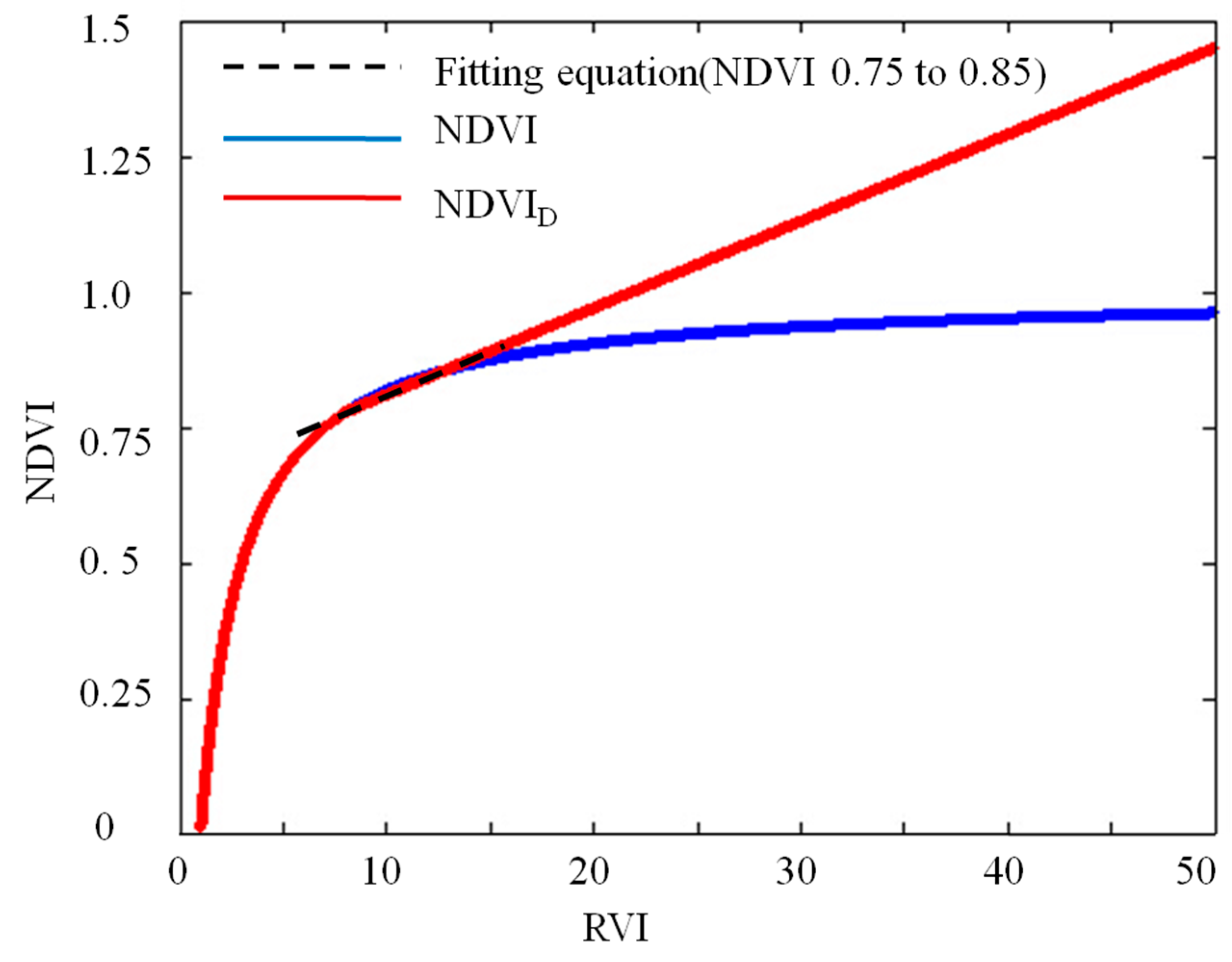
- Thenkabail, P.S.; Smith, R.B.; De Pauw, E. Hyperspectral vegetation indices and their relationships with agricultural crop characteristics. Remote Sens. Environ. 2000, 71, 158–182. [Google Scholar] [CrossRef]
- Mutanga, O.; Skidmore, A.K. Narrow band vegetation indices overcome the saturation problem in biomass estimation. Int. J. Remote Sens. 2004, 25, 3999–4014. [Google Scholar] [CrossRef]
- Santin-Janin, H.; Garel, M.; Chapuis, J.-L.; Pontier, D. Assessing the performance of NDVI as a proxy for plant biomass using non-linear models: A case study on the Kerguelen archipelago. Polar Biol. 2009, 32, 861–871. [Google Scholar] [CrossRef]
- Gu, Y.; Wylie, B.K.; Howard, D.M.; Phuyal, K.P.; Ji, L. NDVI saturation adjustment: A new approach for improving cropland performance estimates in the Greater Platte River Basin, USA. Ecol. Indic. 2013, 30, 1–6. [Google Scholar] [CrossRef]
- Carlson, T.N.; Ripley, D.A. On the relation between NDVI, fractional vegetation cover, and leaf area index. Remote Sens. Environ. 1997, 62, 241–252. [Google Scholar] [CrossRef]
- Li, X.; Cheng, G.; Liu, S.; Xiao, Q.; Ma, M.; Jin, R.; Che, T.; Liu, Q.; Wang, W.; Qi, Y. Heihe Watershed Allied Telemetry Experimental Research (HiWATER): Scientific objectives and experimental design. Bull. Am. Meteorol. Soc. 2013, 94, 1145–1160. [Google Scholar] [CrossRef]
- Kim, G.; Barros, A.P. Downscaling of remotely sensed soil moisture with a modified fractal interpolation method using contraction mapping and ancillary data. Remote Sens. Environ. 2002, 83, 400–413. [Google Scholar] [CrossRef]
- Jin, R.; Li, X.; Yan, B.; Luo, W.; Ma, M.; Guo, J.; Kang, J.; Zhu, Z.; Zhao, S. A nested ecohydrological wireless sensor network for capturing the surface heterogeneity in the midstream areas of the Heihe River Basin, China. IEEE Geosci. Remote Sens. Lett. 2014, 11, 2015–2019. [Google Scholar] [CrossRef]
- Kang, J.; Li, X.; Jin, R.; Ge, Y.; Wang, J.; Wang, J. Hybrid optimal design of the eco-hydrological wireless sensor network in the middle reach of the Heihe River Basin, China. Sensors 2014, 14, 19095–19114. [Google Scholar] [CrossRef] [PubMed]
- Xiao, Q.; Wen, J. HiWATER: Visible and Near-Infrared Hyperspectral Radiometer (7th, July, 2012). Available online: http://dragon2ltc10.westgis.ac.cn/data/f0b641b4-d7a8-4186-a002-7f7078d96103 (accessed on 7 July 2012).
- Xiao, Q.; Wen, J. HiWATER: Thermal-Infrared Hyperspectral Radiometer (10th, July, 2012). Available online: http://card.westgis.ac.cn/data/b26addec-dde4-4a6f-80ef-505041c45a7a (accessed on 10 July 2012).
- Berk, A. Voigt equivalent widths and spectral-bin single-line transmittances: Exact expansions and the MODTRAN®5 implementation. J. Quant. Spectrosc. Radiat. Transf. 2013, 118, 102–120. [Google Scholar] [CrossRef]
- Wang, H.; Xiao, Q.; Li, H.; Zhong, B. Temperature and emissivity separation algorithm for TASI airborne thermal hyperspectral data. In Proceedings of 2011 International Conference on Electronics, Communications and Control (ICECC), Ningbo, China, 9–11 September 2011; pp. 1075–1078.
- Wang, K.; Li, Z.; Cribb, M. Estimation of evaporative fraction from a combination of day and night land surface temperatures and NDVI: A new method to determine the Priestley-Taylor parameter. Remote Sens. Environ. 2006, 102, 293–305. [Google Scholar] [CrossRef]
- Sun, Z.; Wang, Q.; Matsushita, B.; Fukushima, T.; Ouyang, Z.; Watanabe, M. A new method to define the VI-Ts diagram using subpixel vegetation and soil information: A case study over a semiarid agricultural region in the north China plain. Sensors 2008, 8, 6260–6279. [Google Scholar] [CrossRef] [Green Version]
- Nishida, K.; Nemani, R.R.; Running, S.W.; Glassy, J.M. An operational remote sensing algorithm of land surface evaporation. J. Geophys. Res.: Atmos. 2003, 108. [Google Scholar] [CrossRef]
- Jackson, R.D.; Idso, S.; Reginato, R.; Pinter, P. Canopy temperature as a crop water stress indicator. Water Resour. Res. 1981, 17, 1133–1138. [Google Scholar] [CrossRef]
- Chen, C.-F.; Son, N.-T.; Chang, L.-Y.; Chen, C.-C. Monitoring of soil moisture variability in relation to rice cropping systems in the Vietnamese Mekong Delta using MODIS data. Appl. Geogr. 2011, 31, 463–475. [Google Scholar] [CrossRef]
- Rahimzadeh-Bajgiran, P.; Berg, A.A.; Champagne, C.; Omasa, K. Estimation of soil moisture using optical/thermal infrared remote sensing in the Canadian Prairies. ISPRS J. Photogramm. Remote Sens. 2013, 83, 94–103. [Google Scholar] [CrossRef]
- Tucker, C.J. Red and photographic infrared linear combinations for monitoring vegetation. Remote Sens. Environ. 1979, 8, 127–150. [Google Scholar] [CrossRef]
- Gutman, G.; Ignatov, A. The derivation of the green vegetation fraction from NOAA/AVHRR data for use in numerical weather prediction models. Int. J. Remote Sens. 1998, 19, 1533–1543. [Google Scholar] [CrossRef]
- Jiang, L.; Islam, S. Estimation of surface evaporation map over southern Great Plains using remote sensing data. Water Resour. Res. 2001, 37, 329–340. [Google Scholar] [CrossRef]
- World Meteorological Organization (WMO). Guide to Meteorological Instruments and Methods of Observation; WMO-No. 8; WMO: Geneva, Switzerland, 2008. [Google Scholar]
- Lee, T.J.; Pielke, R.A. Estimating the soil surface specific humidity. J. Appl. Meteorol. 1992, 31, 480–484. [Google Scholar] [CrossRef]
- Merlin, O.; Al Bitar, A.; Walker, J.P.; Kerr, Y. An improved algorithm for disaggregating microwave-derived soil moisture based on red, near-infrared and thermal-infrared data. Remote Sens. Environ. 2010, 114, 2305–2316. [Google Scholar] [CrossRef] [Green Version]
- Wagner, W.; Lemoine, G.; Rott, H. A method for estimating soil moisture from ERS scatterometer and soil data. Remote Sens. Environ. 1999, 70, 191–207. [Google Scholar] [CrossRef]
- Verstraeten, W.W.; Veroustraete, F.; van der Sande, C.J.; Grootaers, I.; Feyen, J. Soil moisture retrieval using thermal inertia, determined with visible and thermal spaceborne data, validated for European forests. Remote Sens. Environ. 2006, 101, 299–314. [Google Scholar] [CrossRef]
- Zhihui, W.; Liangyun, L. Monitoring on land cover pattern and crops structure of oasis irrigation area of middle reaches in Heihe River Basin using remote sensing data. Adv. Earth Sci. 2013, 28, 948–956. [Google Scholar]
- Xiao, Q.; Wen, J. HiWATER: Vegetation Height Product in the Middle Reaches of the Heihe River Basin (19 July 2012). Available online: http://dragon2ltc10.westgis.ac.cn/data/6b4f1a86-9b2b-42c3-90e2-6c51358bce69 (accessed on 19 July 2012).
- Weng, Q.; Lu, D. A sub-pixel analysis of urbanization effect on land surface temperature and its interplay with impervious surface and vegetation coverage in Indianapolis, United States. Int. J. Appl. Earth Obs. Geoinf. 2008, 10, 68–83. [Google Scholar] [CrossRef]
- Merlin, O.; Escorihuela, M.J.; Mayoral, M.A.; Hagolle, O.; Al Bitar, A.; Kerr, Y. Self-calibrated evaporation-based disaggregation of SMOS soil moisture: An evaluation study at 3 km and 100 m resolution in Catalunya, Spain. Remote Sens. Environ. 2013, 130, 25–38. [Google Scholar] [CrossRef] [Green Version]
- Sun, Z.; Wang, Q.; Matsushita, B.; Fukushima, T.; Ouyang, Z.; Watanabe, M.; Gebremichael, M. Evaluation of the VI-Ts method for estimating the land surface moisture index and air temperature using ASTER and MODIS data in the North China Plain. Int. J. Remote Sens. 2011, 32, 7257–7278. [Google Scholar] [CrossRef]
- Sharp, R.; Davies, W. Root growth and water uptake by maize plants in drying soil. J. Exp. Bot. 1985, 36, 1441–1456. [Google Scholar] [CrossRef]
- Nemani, R.; Pierce, L.; Running, S.; Goward, S. Developing satellite-derived estimates of surface moisture status. J. Appl. Meteorol. 1993, 32, 548–557. [Google Scholar] [CrossRef]
- Tang, R.; Li, Z.-L.; Tang, B. An application of the Ts-VI triangle method with enhanced edges determination for evapotranspiration estimation from MODIS data in arid and semi-arid regions: Implementation and validation. Remote Sens. Environ. 2010, 114, 540–551. [Google Scholar] [CrossRef]
© 2015 by the authors; licensee MDPI, Basel, Switzerland. This article is an open access article distributed under the terms and conditions of the Creative Commons Attribution license (http://creativecommons.org/licenses/by/4.0/).
Share and Cite
Fan, L.; Xiao, Q.; Wen, J.; Liu, Q.; Tang, Y.; You, D.; Wang, H.; Gong, Z.; Li, X. Evaluation of the Airborne CASI/TASI Ts-VI Space Method for Estimating Near-Surface Soil Moisture. Remote Sens. 2015, 7, 3114-3137. https://doi.org/10.3390/rs70303114
Fan L, Xiao Q, Wen J, Liu Q, Tang Y, You D, Wang H, Gong Z, Li X. Evaluation of the Airborne CASI/TASI Ts-VI Space Method for Estimating Near-Surface Soil Moisture. Remote Sensing. 2015; 7(3):3114-3137. https://doi.org/10.3390/rs70303114
Chicago/Turabian StyleFan, Lei, Qing Xiao, Jianguang Wen, Qiang Liu, Yong Tang, Dongqin You, Heshun Wang, Zhaoning Gong, and Xiaowen Li. 2015. "Evaluation of the Airborne CASI/TASI Ts-VI Space Method for Estimating Near-Surface Soil Moisture" Remote Sensing 7, no. 3: 3114-3137. https://doi.org/10.3390/rs70303114