
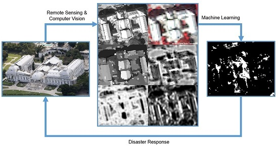
Detection of Urban Damage Using Remote Sensing and Machine Learning Algorithms: Revisiting the 2010 Haiti Earthquake


Abstract
: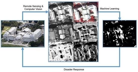
1. Introduction
- Assess the performance of neural networks (to include radial basis function neural networks), and Random Forests on very high resolution satellite imagery in earthquake damage detection
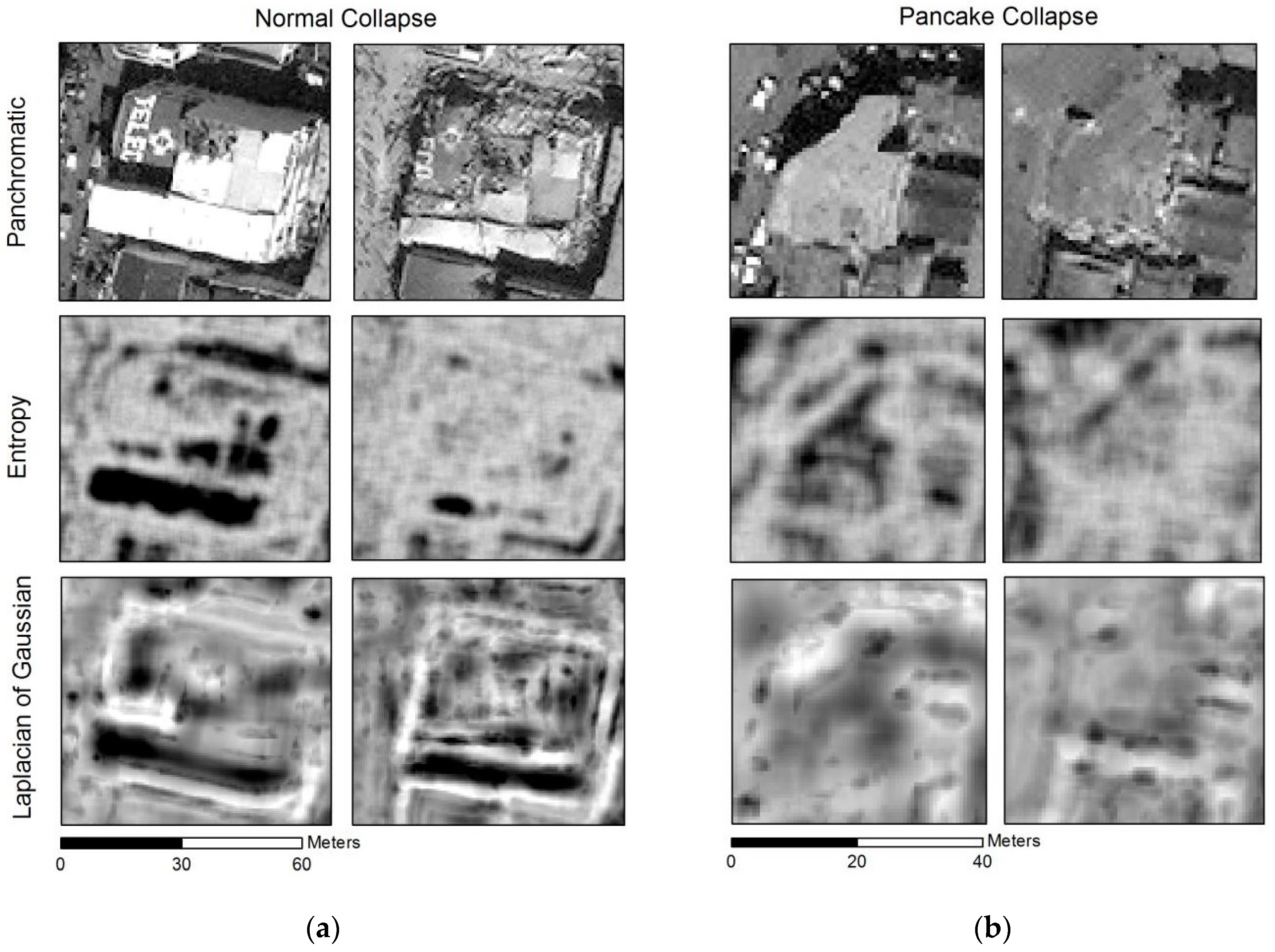
- Investigate the usefulness of structural feature identifiers to include the Laplacian of Gaussian and rectangular fit in identifying damaged regions
2. Materials and Methods
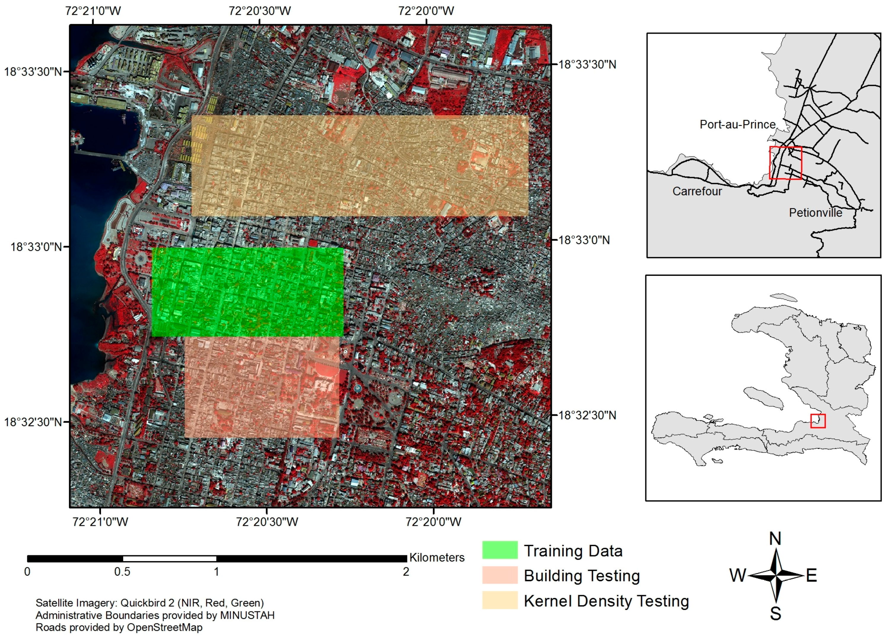
2.1. Study Area and Data
2.2. Texture and Structure
2.3. Machine Learning Algorithms
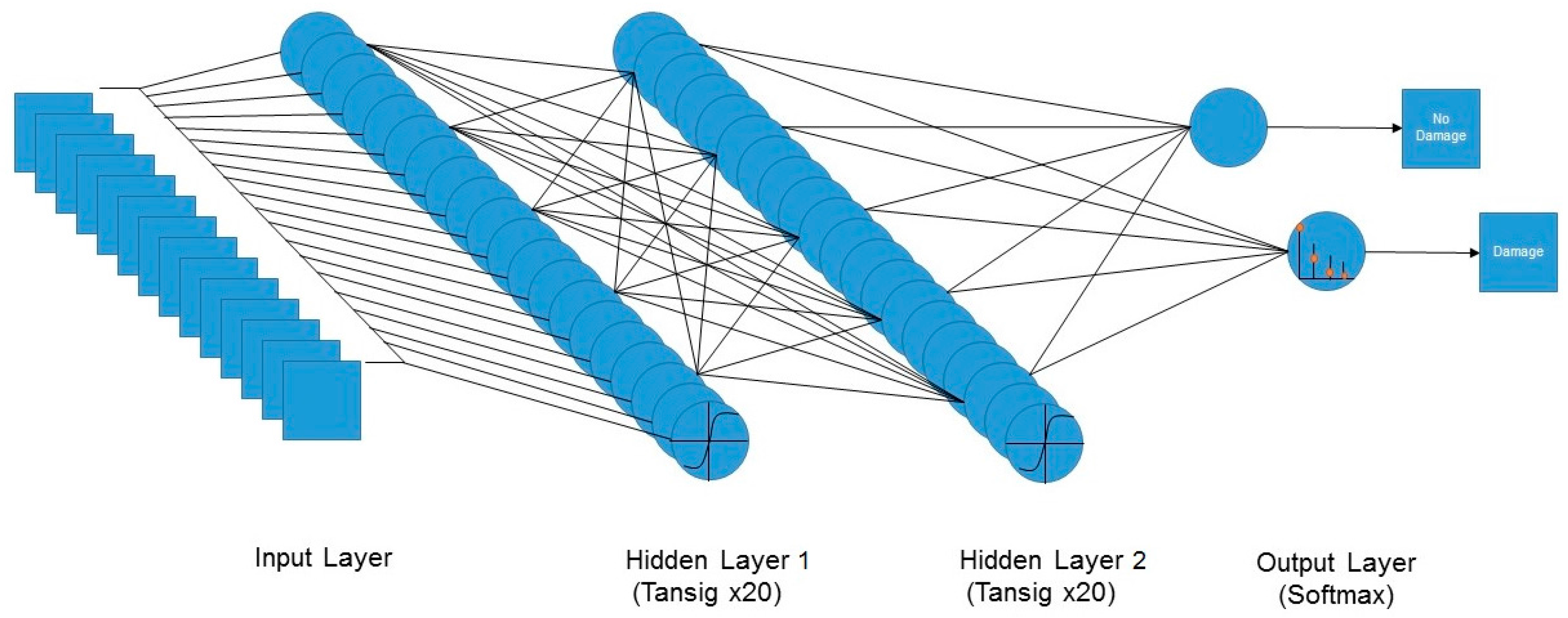
2.3.1. Neural Networks
2.3.2. Random Forests
2.4. Testing and Accuracy Assessement
3. Results
4. Discussion
5. Conclusions
Acknowledgments
Author Contributions
Conflicts of Interest
Appendix A

| Undamaged UNOSAT | Damaged UNOSAT | ANN UA | |
|---|---|---|---|
| Undamaged ANN | 498 | 101 | 83.14 |
| Damaged ANN | 131 | 167 | 56.04 |
| ANN PA | 79.17 | 62.31 | |
| RBFNN UA | |||
| Undamaged RBFNN | 575 | 150 | 79.31 |
| Damaged RBFNN | 54 | 118 | 68.60 |
| RBFNN PA | 91.41 | 44.03 | |
| RF UA | |||
| Undamaged RF | 606 | 191 | 76.04 |
| Damaged RF | 23 | 77 | 77.00 |
| RF PA | 96.34 | 28.73 |
Appendix B
Appendix B.1. Algorithmic Damage Map for the RBFNN Algorithm

Appendix B.2. Algorithmic Damage Map for the Random Forests Algorithm

References
- Dong, L.; Shan, J. A Comprehensive review of earthquake-induced building damage detection with remote sensing techniques. ISPRS J. Photogramm. Remote Sens. 2013, 84, 85–99. [Google Scholar] [CrossRef]
- Ural, S.; Hussain, E.; Kim, K.; Fu, C.; Shan, J. Building extraction and rubble mapping for city Port-au-Prince post-2010 earthquake with GeoEye-1 imagery and Lidar Data. Photogramm. Eng. Remote Sens. 2011, 77, 1011–1023. [Google Scholar] [CrossRef]
- Comfort, L.K. Self Organization in Disaster Response: The Great Hanshin, Japan Earthquake of January 17, 1995; Quick Response Report; Natural Hazards Research and Applications Information Center: Boulder, CO, USA, 1996. [Google Scholar]
- Smith, K. Environmental Hazards, 3rd ed.; Routledge: London, UK, 2001. [Google Scholar]
- Voigt, S.; Schneiderhan, T.; Twele, A.; Gähler, M.; Stein, E.; Mehl, H. Rapid damage assessment and situation mapping: learning from the 2010 Haiti earthquake. Photogramm. Eng. Remote Sens. 2011, 77, 923–931. [Google Scholar] [CrossRef]
- Pham, T.T.H.; Apparicio, P.; Gomez, C.; Weber, C.; Mathon, D. Towards a rapid automatic detection of building damage using remote sensing for disaster management: The 2010 Haiti earthquake. Disaster Prev. Manag. 2014, 23, 53–66. [Google Scholar] [CrossRef]
- Stramondo, S.; Bignami, C.; Chini, M.; Pierdicca, N.; Tertulliani, A. Satellite radar and optical remote sensing for earthquake damage detection: Results from different case studies. Int. J. Remote Sens. 2006, 27, 4433–4447. [Google Scholar] [CrossRef]
- Dell’Acqua, F.; Bignami, C.; Chini, M. Earthquake damages rapid mapping by satellite remote sensing data: L’Aquila April 6th, 2009 event. IEEE J. Sel. Top. Appl. Earth Obs. Remote Sens. 2011, 4, 935–943. [Google Scholar] [CrossRef]
- Gamba, P.; Casciati, F. GIS and image understanding for near-real-time earthquake damage assessment. Photogramm. Eng. Remote Sens. 1998, 64, 987–994. [Google Scholar]
- Goldberg, D.; Holland, J. Genetic algorithms and machine learning. Mach. Learn. 1988, 3, 95–99. [Google Scholar] [CrossRef]
- Xu, J.B.; Song, L.S.; Zhong, D.F.; Zhao, Z.Z.; Zhao, K. Remote sensing image classification based on a modified self-organizing neural network with a priori knowledge. Sens. Transducers 2013, 153, 29–36. [Google Scholar]
- Melgani, F.; Bruzzone, L. Classification of hyperspectral remote sensing images with support vector machines. IEEE Trans. Geosci. Remote Sens. 2004, 42, 1778–1790. [Google Scholar] [CrossRef]
- Benediktsson, J.; Swain, P.H.; Ersoy, O.K. Neural network approaches versus statistical methods in classification of multisource remote sensing data. IEEE Trans. Geosci. Remote Sens. 1990, 28, 540–552. [Google Scholar] [CrossRef]
- Shao, Y.; Lunetta, R.S. Comparison of support vector machine, neural network, and CART algorithm for the land-cover classifcation using limited data points. ISPRS J. Photogramm. Remote Sens. 2012, 70, 78–87. [Google Scholar] [CrossRef]
- Pal, M. Random forest classifier for remote sensing classification. Int. J. Remote Sens. 2005, 26, 217–222. [Google Scholar] [CrossRef]
- Ito, Y.; Hosokawwa, M.; Lee, H.; Liu, J.G. Extraction of damaged regions using SAR data and neural networks. Int. Arch. Photogramm. Remote Sens. 2000, 33, 156–163. [Google Scholar]
- Li, P.; Xu, H.; Liu, S.; Guo, J. Urban building damage detection from very high resolution imagery using one-class SVM and spatial relations. In Proceedings of the IEEE International Geoscience and Remote Sensing Symposium, Cape Town, South Africa, 12–17 July 2009.
- Haiyang, Y.; Gang, C.; Xiaosan, G. Earthquake-collapsed building extraction from LiDAR and aerophotograph based on OBIA. In Proceedings of the 2nd International Conference on Information Science and Engineering, Hangzhou, China, 4–6 December 2010.
- Kaya, G.; Musaoglu, N.; Ersoy, O.K. Damage assessment of 2010 Haiti earthquake with post-earthquake satellite image by support vector selection and adaptation. Photogramm. Eng. Remote Sens. 2011, 77, 1025–1035. [Google Scholar] [CrossRef]
- Li, J.; Du, Q.; Li, Y. An efficient radial basis function neural network for hyperspectral remote sensing image classification. Soft Comput. 2015, 12, 1–7. [Google Scholar] [CrossRef]
- Duda, R.; Hart, P.; Stork, D. Pattern Classification, 2nd ed.; Wiley: New York, NY, USA, 2004. [Google Scholar]
- Kong, H.; Akakin, H.; Sarma, S. A generalized Laplacian of Gaussian filter for blob detection and its applications. IEEE Trans. Cyber. 2013, 43, 1719–1733. [Google Scholar] [CrossRef] [PubMed]
- Ilsever, M.; Ünsalan, C. Two-Dimensional Change Detection Methods; Springer: London, UK, 2012. [Google Scholar]
- Huang, X.; Zhang, L. An adaptive mean-shift analysis approach for object extraction and classification from urban hyperspectral imagery. IEEE Trans. Geosci. Remote Sens. 2008, 46, 4173–4185. [Google Scholar] [CrossRef]
- Li, H.; Gu, H.; Han, Y.; Yang, J. An efficient multiscale SRMMHR (Statistical Region Merging and Minimum Heterogeneity Rule) segmentation method for high-resolution remote sensing imagery. IEEE J. Sel. Top. Appl. Earth Obs. Remote Sens. 2009, 2, 67–73. [Google Scholar] [CrossRef]
- Sun, Z.; Fang, H.; Deng, M.; Chen, A.; Yue, P.; Di, L. Regular shape similarity index: A novel index for accurate extraction of regular objects from remote sensing images. IEEE Trans. Geosci. Remote Sens. 2015, 53, 3737–3748. [Google Scholar] [CrossRef]
- Huang, X.; Zhang, L. Morphological building/shadow index for building extraction from high-resolution imagery over urban areas. IEEE J. Sel. Top. Appl. Earth Obs. Remote Sens. 2012, 5, 161–172. [Google Scholar] [CrossRef]
- Bignami, C.; Chini, M.; Stramondo, S.; Emery, W.J.; Pierdicca, N. Objects textural features sensitivity for earthquake damage mapping. In Joint Urban Remote Sensing Event; Stilla, U., Ed.; Munich: Bavaria, German, 2011. [Google Scholar]
- Marshall, A. How Amateur Mappers Are Helping Recovery Efforts in Nepal. 2015. Available online: http://www.citylab.com/tech/2015/04/how-amateur-mappers-are-helping-recovery-efforts-in-nepal/391703/ (accessed on 15 October 2015).
- Kahn, M.E. The death toll from natural disasters: The role of income, geography, and institutions. Rev. Econ. Stat. 2005, 87, 271–284. [Google Scholar] [CrossRef]
- USGS. Earthquakes with 1000 or More Deaths 1900–2014. Available online: http://earthquake.usgs.gov/earthquakes/world/world_deaths.php (accessed on 19 October 2015).
- Krause, K. Radiometric Use of QuickBird Imagery; DigitalGlobe: Longmont, CO, USA, 2005. [Google Scholar]
- UNITAR/UNOSAT, EC JRC, and World Bank. Haiti Earthquake 2010: Remote Sensing Damage Assessment. Available online: http://www.unitar.org/unosat/haiti-earthquake-2010-remote-sensing-based-building-damage-assessment-data (accessed on 25 September 2015).
- Grünthal, G. European macroseismic scale 1998: EMS-98. Available online: http://www.franceseisme.fr/EMS98_Original_english.pdf (accessed on 20 October 2016).
- Dell’Acqua, F.; Gamba, P. Remote sensing and earthquake damage assessment: Experiences, limits, and perspectives. Proc. IEEE 2012, 100, 2876–2890. [Google Scholar] [CrossRef]
- Tiede, D.; Lang, S.; Füreder, P.; Hölbling, D.; Hoffmann, C.; Zeil, P. Automated damage indication for rapid geospatial reporting: An operational object based approach to damage density mapping following the 2010 Haiti earthquake. Photogramm. Eng. Remote Sens. 2011, 77, 1–10. [Google Scholar] [CrossRef]
- Gebejes, A.; Huertas, R. Texture characterization based on grey-level co-occurrence matrix. In Proceedings of the Conference on Informatics and Management Sciences, Chongqing, China, 16–19 November 2013.
- Miura, H.; Modorikawa, S.; Chen, S.H. Texture characteristics of high-resolution satellite images in damaged areas of the 2010 Haiti earthquake. In Proceedings of the 9th International Workshop on Remote Sensing for Disaster Response, Stanford, CA, USA, 15–16 September 2011.
- Tomowskia, D.; Klonus, S.; Ehlers, M.; Michel, U.; Reinartz, P. Change visualization through a texture-based analysis approach for disaster applications. In Proceedings of the ISPRS TC VII Symposium, Vienna, Austria, 5–7 July 2010.
- Nock, R.; Nielsen, F. Statistical region merging. IEEE Trans. Pattern Anal. Mach. Intell. 2004, 26, 1452–1458. [Google Scholar] [CrossRef] [PubMed]
- Hagan, M.; Demuth, H.B.; Beale, M.H.; De Jesús, O. Neural Network Design, 2nd ed.; PWS Publishing Company: Lexington, KY, USA, 2015. [Google Scholar]
- Shao, Y.; Taff, G.N.; Walsh, S.J. Comparison of early stop criteria for neural network-based sub-pixel classification. IEEE Geosci. Remote Sens. Lett. 2010, 8, 113–117. [Google Scholar] [CrossRef]
- Schwenker, F.; Kestler, H.; Palm, G. Three learning phases for radial-basis-function networks. Neural Netw. 2001, 14, 439–458. [Google Scholar] [CrossRef]
- McCormick, C. Radial Basis Function Network (RBFN). Available online: http://mccormickml.com/2013/08/15/radial-basis-function-network-rbfn-tutorial/ (accessed on 15 February 2016).
- Breiman, L. Random forests. Mach. Learn. 2001, 45, 5–32. [Google Scholar] [CrossRef]
- Breiman, L. Bagging predictors. Mach. Learn. 1996, 24, 123–140. [Google Scholar] [CrossRef]
- Geiss, C.; Pelizari, P.A.; Marconcini, M.; Sengara, W.; Edwards, M.; Lakes, T.; Taubenbock, H. Estimation of seismic building structural types using multi-sensor remote sensing and machine learning techniques. ISPRS J. Photogramm. Remote Sens. 2015, 104, 175–188. [Google Scholar] [CrossRef]
- Witten, I.; Frank, E.; Hall, M. Data Mining, 3rd ed.; Elsevier: Burlington, MA, USA, 2011. [Google Scholar]
- Moller, M.F. A scaled conjugate gradient algorithm for fast supervised learning. Neural Netw. 1991, 6, 525–533. [Google Scholar] [CrossRef]
- Leprince, S.; Barbot, S.; Ayoub, F.; Avouac, J. Automatic and precise orthorectification, coregistration, and subpixel correlation of satellite images, application to ground deformation measurements. IEEE Trans. Geosci. Remote Sens. 2007, 45, 1529–1558. [Google Scholar] [CrossRef]
- Krizhevsky, A.; Sutskever, I.; Hinton, G. ImageNet classification with deep convolutional neural networks. In Proceedings of 26th Annual Conference on Neural Information Processing Systems, Lake Tahoe, NV, USA, 3–8 December 2012.
- Chatfield, K.; Simonyan, K.; Vedaldi, A.; Zisserman, A. Return of the devil in the details: Delving deep into convolutional nets. In Proceedings of the British Machine Vision Conference, Bristol, UK, 9–13 September 2014.
- Vedaldi, A.; Lenc, K. MatConvNet—Convolutional neural networks for MATLAB. In Proceedings of the 23rd ACM international conference on Multimedia, Brisbane, Australia, 26–30 October 2015.


| Sensor | Native Resolution | Acquisition Date | Look Angle |
|---|---|---|---|
| WorldView-1 | 0.5 m panchromatic | 7 December 2009 | 27.62 |
| QuickBird-2 | 2.4 m multispectral 0.6 m panchromatic | 15 January 2010 | 20.7 |
| Remote sensing damage assessment: UNITAR/UNOSAT, EC JRC, World Bank | Vector (point) | 15 January 2010 | N/A |
| Input Feature | Source |
|---|---|
| Panchromatic (450–900 nm) | WV1 and QB2 |
| Entropy | WV1 and QB2 |
| Dissimilarity | WV1 and QB2 |
| LoG | WV1 and QB2 |
| Rectangular fit | WV1 and QB2 |
| Blue (450–520 nm) | QB2 |
| Green (520–600 nm) | QB2 |
| Red (630–690 nm) | QB2 |
| Near infrared (760–900 nm) | QB2 |
| Algorithm | Train + Test Runtime (s) | Overall Accuracy (%) | Building Class Omission Error (%) | Cohen’s Kappa | Kernel Density Match (%) |
|---|---|---|---|---|---|
| ANN | 623 | 74.14 | 37.69 | 0.402 | 87.41 |
| RBFNN | 1532 | 77.26 | 55.97 | 0.3951 | 90.25 |
| RF | 8692 | 76.14 | 71.27 | 0.3057 | 88.77 |
© 2016 by the authors; licensee MDPI, Basel, Switzerland. This article is an open access article distributed under the terms and conditions of the Creative Commons Attribution (CC-BY) license (http://creativecommons.org/licenses/by/4.0/).
Share and Cite
Cooner, A.J.; Shao, Y.; Campbell, J.B. Detection of Urban Damage Using Remote Sensing and Machine Learning Algorithms: Revisiting the 2010 Haiti Earthquake. Remote Sens. 2016, 8, 868. https://doi.org/10.3390/rs8100868
Cooner AJ, Shao Y, Campbell JB. Detection of Urban Damage Using Remote Sensing and Machine Learning Algorithms: Revisiting the 2010 Haiti Earthquake. Remote Sensing. 2016; 8(10):868. https://doi.org/10.3390/rs8100868
Chicago/Turabian StyleCooner, Austin J., Yang Shao, and James B. Campbell. 2016. "Detection of Urban Damage Using Remote Sensing and Machine Learning Algorithms: Revisiting the 2010 Haiti Earthquake" Remote Sensing 8, no. 10: 868. https://doi.org/10.3390/rs8100868