Hyperspectral Sensors as a Management Tool to Prevent the Invasion of the Exotic Cordgrass Spartina densiflora in the Doñana Wetlands

Abstract

We test the use of hyperspectral sensors for the early detection of the invasive dense-flowered cordgrass (Spartina densiflora Brongn.) in the Guadalquivir River marshes, Southwestern Spain. We flew in tandem a CASI-1500 (368–1052 nm) and an AHS (430–13,000 nm) airborne sensors in an area with presence of S. densiflora. We simplified the processing of hyperspectral data (no atmospheric correction and no data-reduction techniques) to test if these treatments were necessary for accurate S. densiflora detection in the area. We tested several statistical signal detection algorithms implemented in ENVI software as spectral target detection techniques (matched filtering, constrained energy minimization, orthogonal subspace projection, target-constrained interference minimized filter, and adaptive coherence estimator) and compared them to the well-known spectral angle mapper, using spectra extracted from ground-truth locations in the images. The target S. densiflora was easy to detect in the marshes by all algorithms in images of both sensors. The best methods (adaptive coherence estimator and target-constrained interference minimized filter) on the best sensor (AHS) produced 100% discrimination (Kappa = 1, AUC = 1) at the study site and only some decline in performance when extrapolated to a new nearby area. AHS outperformed CASI in spite of having a coarser spatial resolution (4-m vs. 1-m) and lower spectral resolution in the visible and near-infrared range, but had a better signal to noise ratio. The larger spectral range of AHS in the short-wave and thermal infrared was of no particular advantage. Our conclusions are that it is possible to use hyperspectral sensors to map the early spread S. densiflora in the Guadalquivir River marshes. AHS is the most suitable airborne hyperspectral sensor for this task and the signal processing techniques target-constrained interference minimized filter (TCIMF) and adaptive coherence estimator (ACE) are the best performing target detection techniques that can be employed operationally with a simplified processing of hyperspectral images.

1. Introduction

The dense-flowered cordgrass (Spartina densiflora Brongn.) is a perennial grass native from salt marshes in the Atlantic coast of South America. It has been accidentally introduced in areas of North America (California and Washington), Europe (Gulf of Cadiz, southwestern Iberian Peninsula) and North Africa (Morocco) where it behaves as an aggressive invader [1]. This cordgrass shows a strong adaptability to environmental conditions, being able to invade a variety of habitats from low unvegetated tidal flats [2] to high topographic elevations in marshes [1]. It grows in dense clumps and represents an extraordinary competitor for native marsh plant species. It can grow in almost mono-specific stands, which simplifies the ecosystem, reducing the richness and diversity of the marsh community [3]. S. densiflora grows in the Gulf of Cadiz showing some of the highest net primary productivity values recorded for the species [4,5], as a proof of its ecological success here.

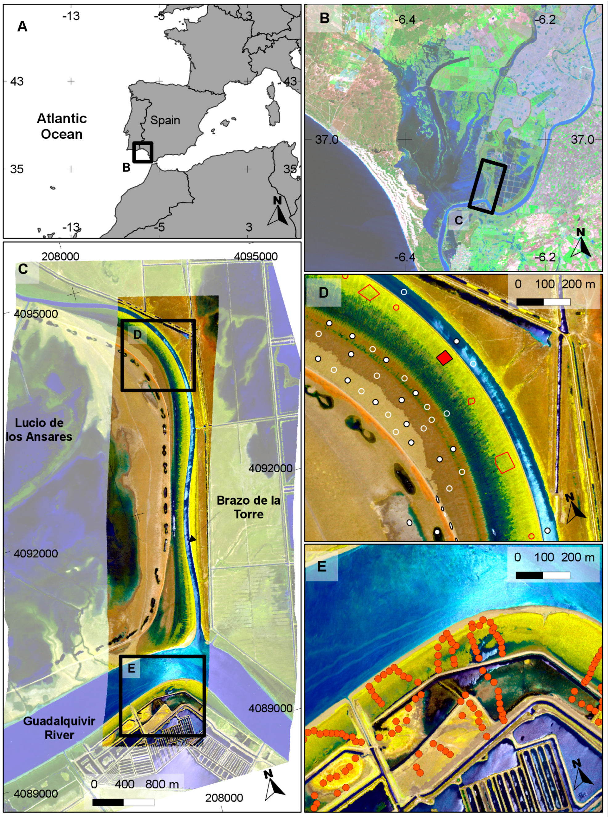
Currently, S. densiflora has expanded along the southern Atlantic coast of the Iberian Peninsula from the Algarve in Portugal to Algeciras Bay (bay of Gibraltar) in Spain, perhaps accidentally introduced to Europe by the lumber trade between South America and Spain in the 16th century [2]. In Doñana National Park, the species has a reduced distribution along the shores of the Guadalquivir River and the banks of some drainage channels. This is due to the “Montaña del Río” dike, an artificial 14-km silt levee that separates the marshes from the Guadalquivir River estuary limiting its expansion farther into the park. Salt-marsh restoration projects in Doñana surroundings have shown that the species can successfully invade if adequate ecological conditions exist [6]. For this reason, it is important to be able to monitor S. densiflora distribution so that adequate eradication measures can be taken before it is too late.

Initiating invasive species control at the beginning of an invasion may be critical for successful eradication of the invaders [7,8]. The evaluation of different techniques to control and eradicate S. densiflora has revealed the difficulty of eliminating the species once established [9], which gives priority toward early detection, as a management tool, in order to act promptly in case of invasion. The doctrine of early detection and rapid response to invasions has been adopted by land and water resource managers, and remote sensing could be the most cost-effective tool for detection [10,11,12]. Therefore, it is essential to establish a system of early prevention, to control the spread of alien species and eradicate them. Remote sensing could facilitate this work, as it can cover large areas like marshes that are difficult to survey on the ground.

Compared to minerals, spectral separability of plants at the species level presents unique challenges. Reflectance spectra of plants in the visible wavelengths are mainly determined by the concentration of different pigments present in all species: chlorophylls a and b and carotenoids, while in the near infrared they are mainly influenced by the disposition of air spaces in the leaf structure [13]. In addition, there is spectral variability within species and there is seasonal variation in aspects that influence reflectance spectra, like pigment concentration and leaf area index. This can be a limitation, or can be used for species identification by using the differences among species in temporal changes of spectral signatures [14]. In spite of these shortcomings, remote sensing has proved to be a cost-effective tool for studies on vegetation distribution [15,16], and in particular, for the detection and mapping of invasive species [10,17,18,19,20,21,22,23,24,25,26,27,28]. Some studies have used low spatial resolution images such as Landsat TM [14] or Hyperion [25,29]. However, in the initial stages vegetation patches of invasive species can be small and difficult to detect with medium resolution satellite sensors [30]. So currently, high spatial resolution images from satellite or airborne sensors are needed for early detection [23,24].

Analysis of hyperspectral images taken from airborne sensors is complex and there are no easy well tested protocols for invasive species detections. There are a variety of hyperspectral sensors that have been tested with invasive species: like AVIRIS [19,20], CASI [31,32,33,34], Probe-1 [21,22], Hymap [10,26,28,35], SOC-700 [23], and PHILLS II [24]. Images need to be corrected for geometric and atmospheric effects [23,24,35]. Numerous classification and detection algorithms have been used including supervised and unsupervised classification techniques [27], spectral linear unmixing [24], classification and regression trees [22,26], spectral angle mapper [20,36], neural networks [33], and matched filters [28]. It is common to perform data reduction techniques like Principal Component Analysis (PCA) or Minimum Noise Fraction (MNF) on the band raw data [19,24,25], to work with band indexes, or with a certain selection of bands. Success is variable depending not only on the species but on the mixture of other species present [26]. All this probably precludes a more extensive operational use of hyperspectral remote sensing for invasive species monitoring by environmental managers.

We wanted to test if it was possible to detect S. densiflora with hyperspectral sensors in the marshes of Doñana National Park using relatively easy and fast processing techniques that could be used operationally for early detection and monitoring of the invasion progress. For that purpose, we planned to reduce data processing to the minimum and work with raw radiance images without data reduction techniques. Atmospheric correction is not essential for target discrimination if training spectra are taken from the image using ground-truth locations [25]. We flew in tandem two airborne hyperspectral sensors: CASI-1500, which had already been used for invasive species detection [31,32,33,34,37] and AHS, which has not been tested for that purpose, although it has proved successful for plant species discrimination [38]. Being flown in tandem, atmospheric influence is similar on the spectra recorded by both sensors and atmospheric correction can be avoided if we want to compare target discrimination ability. We tested the comparative success of several spectral target detection techniques that are integrated in ENVI version 4.6.1. (Exelis Visual Information Solutions, Boulder, Colorado) Target Detection Wizard that guides step by step the user in the detection of the targets of interest [39] and that can be easily applied by non-specialists in remote sensing.

2. Study Area

The study was conducted in Doñana National Park (53671 ha), Southwestern Spain (Figure 1). The area is a seasonal freshwater marsh at the mouth of the Guadalquivir River. The variable winter rainfall yearly floods the Doñana marshes forming a wide shallow lake that dries up during spring and summer. Flooded areas are very variable in depth and turbidity, being driven by the amount and seasonal pattern of rainfall. Some areas in the southeastern part of the park have tidal influence and salt-marsh vegetation in which S. densiflora is present, sometimes in dense monospecific narrow bands along the banks of the river and marsh drainage channels and sometimes mixed with other salt-marsh vegetation. During the inundation period, submerged, floating and emergent plant species grow to fully cover certain areas. Dominant and native emergent species are Bolboschoenus maritimus, Scirpus littoralis, Juncus subulatus and Arthrocnemum macrostachyum. Among the diverse submerged plant community, Ranunculus peltatus, Myriophyllum alterniflorum, Chara gallioides and Ruppia drepanensis are the most abundant. For a more detailed description see the works by Espinar et al., García-Murillo et al. and Rivas Martínez et al. [40,41,42]. We selected an area of 763 ha along the lower banks of the “Brazo de la Torre” channel where it meets the Guadalquivir River (Figure 1C) that had been covered by two hyperspectral sensors flown in tandem for vegetation mapping purposes and we had collected ground-truth field data of S. densiflora distribution on the same year. The study area corresponds to the overlap of the footprint of both sensors from a single flight-line (Table 2). All necessary permits were obtained for field sampling in Doñana National Park as well as for the hyperspectral flights over the protected area. Permits were issued by the Director of Espacio Natural Doñana, Dirección General de Espacios Naturales y Participación Ciudadana, Consejería de Medio Ambiente, Junta de Andalucía. No field specimens were collected.

3. Material and Methods

3.1. Hyperspectral Images

An airborne remote sensing campaign was carried out over Doñana National park by the Instituto Nacional de Técnica Aeroespacial (INTA) on the 21 May 2011 for vegetation mapping purposes. Two hyperspectral sensors (a CASI-1500 and an AHS) were flown in tandem on a high-wing twin-engine turboprop unpressurized airplane CASA-212-200. Both sensors were connected to an Inertial Measurement Unit (IMU) GPS/INS POS-AV 410 manufactured by Applanix (http://www.applanix.com) that provides sensor position and attitude during image acquisition [43]. Images were pre-processed by INTA. They were radiometrically corrected to at-sensor spectral radiance and geometrically corrected using IMU data and the Andalusian GPS Network (www.juntadeandalucia.es/obraspublicasytransportes/redandaluzadeposicionamientorap) with a mean position error (RMS) below 1 pixel [44].

One of our aims was to test if detection analyses performed on images at sensor radiance without any atmospheric correction, and without any data reduction techniques (like PCA or MNF) performed well enough. Both sensors were flown in tandem (so were similarly affected by the atmosphere), image spectra taken from ground-truth targets were used for training the target detection algorithms, and no extrapolation was planned for images from different dates or in different areas with no ground-truth. Under these circumstances it is not necessary to transform the images to ground reflectances performing an atmospheric correction [25], and image processing is simplified.

There are three methods for atmospheric correction implemented in ENVI: Quick Atmospheric Correction (QUAC, [45,46]), Fast Line-of-Sight Atmospheric Analyses of Spectral Hypercubes (FLAASH, [47]) and Empirical Line Correction (ELC, [48]). They differ in the amount external information required to correct the images and the degree of expertise required to apply the method. These methods are only adequate to correct images in the VNIR and SWIR ranges of the spectrum. TIR images (AHS) can be corrected in ENVI with the Thermal Atmospheric Correction and transformed into emissivity images bands and a thermal image with three methods: Emissivity Reference Channel, Emissivity Normalization or Emissivity Alpha Residuals. It is not the aim of this paper to test if all atmospheric correction methods produce the same result, or which data reduction technique is optimal. To test if atmospheric correction or data reduction techniques improved Spartina detection we run all models also on atmospherically corrected images with MNF transformation, and compared the performance to that of uncorrected raw bands.

The CASI 1500i (Compact Airborne Spectrographic Imager) is a “pushbroom” radiometer designed and manufactured by ITRES Inc. (http://www.itres.com). The image is generated by a bidimensional array of CCDs by means of the relative movement of the plane over the terrestrial surface. It has up to 288 spectral bands with high spatial and spectral resolution covering the visible and near infrared (VNIR) parts of the electromagnetic spectrum, 368–1052 nm.

The AHS is a “line-scanner” radiometer with 80 spectral bands, designed and manufactured by SenSytech Inc. (currently Argon ST, http://www.argonst.com, and previously Daedalus Ent. Inc.) [49]. It has a 45° rotating mirror that generates the scan lines. It has a coverage in the VNIR from 430–1000 nm with relatively wide bands (27–30 nm). In the SWIR it has a single band centered on 1600 nm. Then it has narrow bands (13 nm) in the MIR region between 2000 and 2500 nm, and in the TIR has a high spectral resolution (between 300 and 500 nm), covering completely both atmospheric transmissivity windows from 3000 to 5000 nm and from 8000 to 13,000 nm. The technical details of the airborne campaign and of both sensors are given in

Table 1. Summary of acquisition parameters of airborne campaign.

	Value
Flight altitude	1844 m (asl)
Terrain altitude	0–10 m (asl)
Date	21 May 2011
Time (UTC)	12:29
Time (local)	14:29
Flight course	169°
Flight-line ID	20110521D-18.7-P25
length/duration	13.5 km/187 s

and

Table 2. Technical characteristics of hyperspectral sensors used for S. densiflora mapping.

Sensor	CASI	AHS
FOV	0.698 rad (40°)	1.571 rad (90°)
IFOV	0.49 mrad	2.5 mrad
Pixels per line	1441	750
Swath	1635 m	3678 m
GSD, pixel size	~1 m	~4 m
VNIR range	360–1052 nm	430–1000 nm
(No. bands)	(144)	(20)
VNIR FWH	2.75 nm	27–30 nm
SWIR range	-	1600 nm
(No. bands)		(1)
SWIR FWHM	-	85 nm
MIR range	-	2000–2500 nm
(No. bands)		(42)
MIR FWHM	-	14–18 nm
TIR range	-	3000–13,000 nm
(No. bands)		(17)
TIR FWHM	-	288–556 nm
AHS scan frequency	-	18.7 rps
analog to digital conversion	14 bit	12 bit

, respectively.

AHS and CASI images differ not only in spectral resolution and spectral range but also in spatial resolution (4-m vs. 1-m). To be able to compare both sensors we generated three new hyperspectral images: CASI-4m (by resampling the CASI image to the spatial resolution of the AHS image), CASI-4m-SR (resampling the CASI image to the spatial and the spectral resolution of the AHS image) and AHS-4m-SR (selecting the AHS bands in the range that both sensors overlap in the VNIR range, 430–1000 nm, and masking the image to the spatial extent of the CASI image). The spatial resolution of an airborne campaign is something can be modified by deciding flying altitude, but a higher resolution increases flight duration and campaign cost. The new CASI-4-m pixel had the average radiance of 16 pixels of the original CASI image. The “4m-SR” images had 20 spectral bands at the spectral resolution of the AHS sensor (VNIR FWH 27–30 nm) in the spectral range 430–1000 nm where both sensors overlap (Table 2), at the spatial resolution of the AHS sensor (4-m), and masked to the area of the CASI footprint (Figure 1C).

3.2. Atmospheric Correction and Data Reduction

All images were atmospherically corrected in the VNIR, SWIR, and MIR ranges (360–2500 nm) using the Quick Atmospheric Correction implemented in ENVI. QUAC is a VNIR-SWIR atmospheric correction method for hyperspectral images. Unlike other first-principles atmospheric correction methods, it determines atmospheric compensation parameters directly from the information contained within the scene (observed pixel spectra), without ancillary information.

This makes the method particularly adequate for inexperienced users as no parameters have to be provide to the program. QUAC performs a more approximate atmospheric correction than FLAASH or other physics-based first-principles methods, generally producing reflectance spectra within approximately ±15% of the physics-based approaches. QUAC is based on the empirical finding that the average reflectance of a collection of diverse material spectra, such as the endmember spectra in a scene, is essentially scene-independent. All of this means significantly faster computational speed compared to the first-principles methods [45,46].

The TIR bands in the AHS image (3000–13,000 nm) cannot be atmospherically corrected in this way. The atmospheric correction algorithm used in ENVI is similar to the In-Scene Atmospheric Compensation algorithm, ISAC [50]. This algorithm assumes that the atmosphere is uniform over the data scene and that a near-blackbody surface exists within the scene. The location of the blackbody surface in the scene is not required for this correction. A single layer approximation of the atmosphere is used. No reflected downwelling radiance is also assumed. The algorithm first determines the wavelength that most often exhibits the maximum brightness temperature. This wavelength is then used as the reference wavelength. Only spectra that have their brightest temperature at this wavelength are used to calculate the atmospheric compensation. At this point, for each wavelength, the reference blackbody radiance values are plotted against the measured radiances. A line is fitted to the highest points in these plotted data and the fit is weighted to assign more weight to regions with denser sampling. The compensation for this band was then applied as the slope and offset derived from the linear regression of these data with their computed blackbody radiances at the reference wavelength. Upwelling atmospheric radiance and atmospheric transmission were approximated using the following method. First, the surface temperature of every pixel was estimated from the data and used to approximate the brightness temperature using the Planck function and assuming an emissivity of 1. Next, a line was fitted using the “Top of Bins” method that fits a standard least squares regression on the top 5% of the data in the scatter plot of radiance vs. brightness temperature. The atmospheric upwelling and transmission are then derived from the slope and offset of this line [50].

The radiation emitted from a surface in the thermal infrared wavelengths is a function of both the surface temperature and emissivity. To calculate emissivity we used the Emissivity Normalization method. This technique calculates the temperature for every pixel and band in the data using a fixed emissivity value provided by the user (we used 0.98). The highest temperature for each pixel is used to calculate the emissivity values using the Planck function.

We used the Minimum Noise Fraction (MNF) transform on the atmospherically corrected images before applying the target detection models. ENVI uses the MNF transform to segregate and equalize the noise in the data, and to reduce the data dimensionality for target detection processing. The resulting bands of the MNF transformed data are sorted by spatial coherence in descending order. Lower MNF bands typically have spatial structure and contain most of the information while higher MNF bands typically have little spatial structure and contain most of the noise [51]. It is frequently assumed that fitting models with all bands will produce overfitted models that will not perform well when extrapolated to a new area.

3.3. Spectral Target Detection Algorithms

Spectral target detection refers to the identification of a particular spectral signature in high spectral resolution remotely sensed images to map the locations of a target (often a mineral or a plant species) of interest. Spectral target detection encompasses a broad range of algorithms designed to pick up the signal of a certain spectrum in a mixture with other undesired target spectra and noise. There are different methods available. Spectral correlation, spectral angle mapper, or linear spectral mixture analysis are well-known techniques that have been employed for plant species detection and classification [20,25,52]. More recent methods derive from statistical signal processing [53] in which the target signal is modeled as a function consisting of both a deterministic and a stochastic (random) component. Statistical signal processing methods are used in fields ranging from identification of targets with radar [54] to speech recognition [55]. These methods do not require unrealistic amounts of a priori information and are known as hyperspectral signal processing techniques [53]. Six target detection algorithms were tested to map S. densiflora distribution in the study area. They were selected because they are the algorithms implemented in the “target detection wizard” module of ENVI [39]. This is an ENVI module that guides the user and requires very limited remote sensing expertise to be used. Some of the algorithms like Spectral Angle Mapper (SAM) and Matched Filtering (MF) are well-known and have been tested for the identification of invasive species with hyperspectral images [20,28,36] while Constrained Energy Minimization (CEM), Adaptive Coherence Estimator (ACE), Orthogonal Subspace Projection (OSP), and Target-Constrained Interference-Minimized Filter (TCIMF) derive from statistical signal processing and have received little attention yet in the invasive species detection literature. The algorithms we tested were:

• Spectral Angle Mapper (SAM): SAM is a widely used spectral similarity measure in remote sensing and has been used for plant species discrimination [20,25,35,36,56,57,58,59]. This algorithm estimates the similarity between two spectra by calculating the angle between them in the multidimensional space defined by the spectral bands [60]. The smaller the angle the greater the similarity. The SAM algorithm is relatively insensitive to differences in brightness so that the same spectra in the shade or under direct sunlight will still have a small spectral angle and a high similarity.
• Matched Filtering (MF): Matched filtering is a technique of applying a finite-impulse response filter to an unknown spectrum to try to detect the presence of a target in the presence of noise. The matched filter is the optimal linear filter for maximizing the signal to noise ratio in the presence of additive stochastic noise. Matched filters were invented by North in 1943 to detect radar signals in the presence of white noise, but since then, have been used as a signal detection technique in many areas like hyperspectral remote sensing. Matched filters have been also used for plant species detection.
• Constrained Energy Minimization (CEM): CEM was first proposed by Harsanyi in 1993 [61] and published in 1994 [62]. CEM requires the knowledge of the spectrum target that needs to be identified and uses a finite-impulse response (FIR) filter to pass through the desired target while minimizing its output energy resulting from a background other than the desired target [53]. A correlation or covariance matrix is used to characterize the composite unknown background. CEM is similar to MF in that the only required knowledge is the target spectrum to be detected. In a mathematical sense, MF is a mean-centered version of CEM, where the data mean is subtracted from all pixel vectors [39].
• Adaptive Coherence Estimator (ACE): ACE is derived from the Generalized Likelihood Ratio (GLR) approach [63]. The ACE is invariant to relative scaling of target spectrum and has a Constant False Alarm Rate with respect to such scaling. Similar to CEM and MF, ACE does not require knowledge of all the endmembers within an image scene [39].
• Orthogonal Subspace Projection (OSP): The OSP approach was first proposed by Harsanyi and Chang [64]. They assumed that if there was a target spectrum among undesired targets, all undesired targets could be considered as interferers. In this case, an unconstrained orthogonal subspace projection eliminated the interfering effects caused by the undesired targets before the detection took place. As a consequence of annihilation of undesired targets the detectability of the desired target spectrum was improved [53]. In ENVI, an orthogonal space projection is defined to eliminate the effect of undesired targets and then a MF is applied to detect the desired target [39]. Therefore, at least one undesired target spectrum (or background spectrum in our terminology) has to be provided apart of the desired target spectrum.
• Target-Constrained Interference-Minimized Filter (TCIMF): The TCIMF assumes that a hyperspectral image scene is made of three separate signal sources: desired targets, undesired targets and interference [53]. The CEM filter takes care of the interference problem. The OSP filter takes care of the undesired target problem. The TCIMF algorithm resolves both problems simultaneously: constrains the desired and undesired spectra in such a way that the desired target spectrum can be detected while suppressing the interference [53]. The procedure is implemented in ENVI and at least one desired spectrum and one undesired spectrum (or background spectrum) have to be provided [39].

3.4. Ground Truth Data, Model Training and Model Validation

The right bank of the Guadalquivir River and the “Brazo de la Torre” had been photo-interpreted by a vegetation expert using aerial photos of summer 2010 to delineate S. densiflora stands (Figure 1C). The area had also been visited in 2011 before the flight to locate S. densiflora patches and isolated clumps. As S. densiflora tends to grow in dense bands along the river bank we decided to delineate with differential GPS (Leica 1200) polygons that had a uniform monospecific and high percent cover of S. densiflora and also monospecific polygons of other marsh species with which it grows in mixed stands in the area. As the sample size of field-delineated polygons of other marsh plant species and other undesired targets in the area covered simultaneously by the footprints of both hyperspectral images was small, we photo-interpreted a false color composition of the CASI-1500 image (RGB = 861.6, 650.8, 550.1 nm). We delineated polygons for undesired targets that were dominant in the area like: glasswort vegetation (mainly Sarcocornia perennis and Arthrocnemum macrostachyum), bare dry soil, mud, open water deep and shallow, and also some extra polygons of S. densiflora (Figure 1D,

Table 3. Ground-truth polygons used for training the spectral detection algorithms (training set) and for validation (testing set).

Class	Cover Type	GPS	Photo-Interpreted	Total	Training Set	Testing Set
T	S. densiflora > 80% cover	7	8	15	7	8
B	Arthrocnemum ~50% cover	2	7	9	4	5
	Sarcocornia ~50%–80% cover	7	33	40	20	20
	Wet bare soil	0	15	15	7	8
	Dry bare soil	0	36	36	18	18
	Water	0	36	36	18	18
Total		16	135	151	74	77

Ground-truth polygons were either delineated with differential GPS in the field selecting vegetated areas with homogeneous and monospecific cover or photo-interpreted on a false-color composition of the CASI image. Only Spartina densiflora monospecific polygons were used as target (Class T) and the remaining polygons of undesired targets were grouped as background (Class B). Polygons were splitted at random in a training set (used to train the target detection models) and a testing set (used for model validation).

).

3.5. Model Training

In our detection problem we had a single “desired target” that was S. densiflora while all other spectra present in the images were considered “undesired targets” (other plant species, bare soil, open water). The “desired target” is referred hereafter as “target” while the “undesired targets” are grouped and referred hereafter as “background”. We randomly selected half of the target polygons delineated with GPS and half of the target polygons photo-interpreted in the image as training set (7 polygons, see Table 3), and used them to obtain a spectral signature from each of the hyperspectral images (CASI, CASI-4m, CASI-4m-SR, AHS, and AHS-4m-SR). These mean spectral signatures were used as the target to train the spectral detection algorithms (Figure 2 and Figure 3). All other ground-truth cover types were considered as background, and a spectral signature was extracted from each of the images with half of these polygons selected at random (67 polygons, Table 3). The algorithms SAM, MF, CEM, and ACE only require a target spectrum and used the spectrum extracted from the 7 target training polygons. While OSP and TCIMF require both a target and a background spectrum and used the 74 polygons of the training set.

The target detection was applied using ENVI “target detection wizard” module [39]. This module produces a rule-image for each combination of detection algorithm and hyperspectral image and a cut-point to classify pixels into target or background. Rule-image values depend on the algorithm used and are not directly comparable. The default cut-points selected by ENVI for each algorithm were not optimal in our setting. A different cut-point for each model can be provided by the user. In order to compare the models in a fair setting we selected cut-points with the same criterion for all algorithms (Tables S1 and S2, Supplementary Material). We extracted the rule-image values from each model using the target and background polygons from the training set. We selected as new cut-point the mid-point between the upper-limit of the 95% confidence interval of the background class and the lower-limit of the 95% confidence interval of the target class (Figure 4).

3.6. Model Validation

Testing polygons are the target and background polygons not used for model training (Table 3) and were used for testing or validation of the models. They were rasterized at the resolution of each image and individual pixels were classified as target or background according to the rule-image value and cut-point for each model. From these data we calculated commission and omission errors for the target, correct classification rate, Cohen’s Kappa, and the AUC (Area Under the Curve) of a ROC (Receiver-Operator Characteristics) plot. Correct classification rate is presented to be able to compare our results with other published papers on invasive species detection, but is an unreliable performance indicator with unequal sample sizes, while Cohen’s Kappa and AUC are unbiased estimators of model reliability. Cohen’s Kappa is influenced by cut-point selection while AUC is not. User’s and producer’s accuracy, which are terms common in the remote sensing literature, can be derived from commission and omission errors: User’s accuracy = (1 − commission error) and producer’s accuracy = (1 − omission error). In our detection problem, omission error (1 − producer’s accuracy) is more relevant and something a manager would like to minimize, so that no populations of the invasive species are left unidentified.

3.7. Model Evaluation at a Different Area

As the predictions of different models tended to agree spatially (Figure 5), and we were interested whether the models could be extrapolated outside the training area, we selected a second area for model evaluation on the left bank of the Guadalquivir River in the place known as “Codo de la Esparraguera “(Figure 1E). This area has S. densiflora populations, but we had no ground-truth data previous to the flight and no photo-interpretation of vegetation had taken place in 2010. We identified areas in which models differed in their predictions, as indicated by the rule-images resulting from the ENVI “Target Detection Wizard”, and used them to focus field-work sampling where model predictions tended to differ. The area was visited on the 7 May 2012. We performed linear transects with a total of 129 sampling points separated by a minimum distance of 20 m and covering areas with and without S. densiflora. We visually estimated, in a 2 m radius circle around the sampling point, the percent ground cover of S. densiflora in a semi-quantitative scale from 0 to 6 (0 = absence, 1 = presence < 5% cover, 2 = 5%–25%, 3 = 25%–50%, 4 = 50%–75%, 5 = 75%–99%, 6 = 100%). Other marsh vegetation species recorded at sampling points were Arthrocnemum macrostachyum, Tamarix africana. Suaeda vera, Phragmites australis, Sarcocornia perennis, Bolboschoenus maritimus, and Juncus acutus. The points were georeferenced with a navigation GPS with 2 m location precision. As both algorithm prediction and field evaluation data are in a quantitative scale we calculated the Spearman rank correlation between S. densiflora coverage at the sampling point and the value at the corresponding pixel of the rule-image for each target detection algorithm (SAM, MF, CEM, ACE, OSP, and TCIMF) and hyperspectral image (CASI, CASI-4m, CASI-4m-SR, AHS, and AHS-4m-SR). We also calculated the AUC of the ROC plot for each combination of the semi-quantitative coverage classes to determine to what extent the cover classes could be differentiated by the models. In order to compare the classification accuracy of each model with that obtained previously for the test polygons (validation), and with accuracy assessment provided in other studies, we reclassified sampling points as S. densiflora presence (cover > 50%, classes 4–6) and S. densiflora absence (class 0) and then calculated the AUC of the ROC plot, Kappa, correct classification rate, omission and commission errors.

3.8. Statistical Analyses

To test the relative importance of sensor, spatial resolution, spectral resolution, atmospheric correction, and detection algorithm we fitted a Generalized Linear Model (GLM) to the Spearman rank correlation of each model prediction with S. densiflora cover at sampling points at the evaluation site of “Codo de la Esparraguera”using normal errors and identity link. Models were fitted in R 3.2.5 [65]. Significance of each factor and interaction between atmospheric correction and detection algorithm was tested by model simplification, starting from the full model.

4. Results

4.1. Prediction of S. densiflora Distribution

The distribution of S. densiflora in the study area as predicted by each model (combination of image and detection algorithm) is shown in Figure 5. All models, in general, agree predicting the presence of S. densiflora growing as a dense band along the shores of the Guadalquivir River and the “Brazo de la Torre” channel (Figure 5). This distribution also agrees quite precisely, on the right banks of the Guadalquivir River and “Brazo de la Torre” channel, with a previous photo-interpretation of the vegetation using aerial photos from summer 2010 (Figure 6). As S. densiflora is a perennial grass no large changes in distribution take place in a year and this can be used a qualitative validation of the models. The left banks, outside Doñana National Park, were not photo-interpreted and so there is no S. densiflora distribution with which to compare.

4.2. Model Validation

All target detection algorithms were able to identify S. densiflora in the CASI image. Cut-points selected by ENVI for each algorithm were not necessarily optimal. For example, for ACE a cut-point of 0.65 was selected by default by ENVI and this cut-point did not identify S. densiflora in the image, but the rule-image suggested that areas with S. densiflora had higher values than the background. By using a different cut-point (see methods, Figure 4) ACE identified the S. densiflora target in a similar way as the other algorithms did.

Table 4. Total area covered by S. densiflora in ha. As predicted by each spectral detection algorithms on the different hyperspectral images used.

	Hyperspectral Image (1)
Algorithm (2)	CASI (3)	CASI-4m	CASI-4m-SR	AHS	AHS-4m-SR
SAM	84.49	80.11	84.57	80.47	82.64
MF	92.65	77.23	97.28	84.35	91.19
CEM	93.34	77.89	97.70	84.36	91.84
ACE	111.58	115.72	85.67	54.22	75.40
OSP	92.15	88.39	90.18	87.88	88.56
TCIMF	94.01	79.61	99.01	83.55	92.15

⁽¹⁾ CASI: image at the original resolution of 1 m, CASI-4m: CASI image resampled at resolution of the AHS (4 m). CASI-4m-SR: CASI image at the spatial and spectral resolution of AHS. AHS: original AHS image. AHS-4m-SR: AHS bands in the VNIR that overlap the spectral range of CASI masked to the area of spatial overlap of both sensors; ⁽²⁾ Algorithms: SAM = Spectral Angle Mapper, MF = Matched Filter, CEM = Constrained Energy Minimization, ACE = Adaptive Coherence Estimator, OSP = Orthogonal Subspace Projection, TCIMF = Target-Constrained Interference-Minimized Filter; ⁽³⁾ Surface, in ha, classified as S. densiflora in the 763 ha that correspond to the area of overlap of both sensors.

shows the extent of the area identified as S. densiflora by each algorithm and hyperspectral image combination. The cut-points selected are provided in Supplementary Material.

Table 5. Validation of the prediction of the spectral detection algorithms using the test polygons in each hyperspectral image.

Sensor (1)	Algorithm (2)	OE (%) (3)	CE (%)	CCR (%)	K	AUC
CASI	SAM	13.35	0	95.03	0.8907	0.9986
	MF	0.24	0.72	99.64	0.9923	0.9999
	CEM	0.19	0.87	99.60	0.9915	0.9999
	ACE	0.05	5.26	97.91	0.9559	0.9999
	OSP	2.64	0	99.02	0.9789	0.9986
	TCIMF	0.21	0.61	99.69	0.9935	0.9999
CASI-4m	SAM	20.45	0	92.57	0.8320	0.9989
	MF	2.74	2.74	98.00	0.9569	0.9989
	CEM	2.74	2.74	98.00	0.9569	0.9989
	ACE	0.17	11.82	95.07	0.8964	0.9980
	OSP	2.92	0	98.94	0.9769	0.9991
	TCIMF	2.06	2.39	98.38	0.9650	0.9992
CASI-4m-SR	SAM	18.18	0	93.38	0.8513	0.9989
	MF	0	0.29	9981	0.9960	1
	CEM	0	0.29	99.81	0.9960	1
	ACE	0.17	0	99.94	0.9987	1
	OSP	2.74	0	99.00	0.9783	0.9994
	TCIMF	0	0.29	99.81	0.9960	1
AHS	SAM	13.19	0	93.04	0.8429	0.9999
	MF	0	0	100	1	1
	CEM	0	0	100	1	1
	ACE	4.40	0	98.40	0.9651	1
	OSP	2.11	0	99.23	0.9833	0.9999
	TCIMF	0	0	100	1	1
AHS-4m-SR	SAM	19.04	0	93.07	0.8440	0.9996
	MF	0	0	100	1	1
	CEM	0	0	100	1	1
	ACE	0.17	0	99.94	0.9987	1
	OSP	2.92	0	98.94	0.9769	1
	TCIMF	0	0	100	1	1

⁽¹⁾ Statistical validation at the pixel level with 77 test polygons (Table 3). CASI image at the original resolution of 1 m, sample size: target n = 9244 pixels, background n = 15599 pixels. CASI-4m: CASI image resampled at the resolution of the AHS image (4 m), sample size: target n = 582 pixels, background n = 1019 pixels. AHS image at the original resolution of 4 m, sample size: target n = 568 pixels, background n = 997 pixels. CASI & AHS-4m-SR images at 4m resolution in the area of spatial and spectral overlap sample size: target n = 583 pixels, background n = 1019 pixels; ⁽²⁾ AM = Spectral Angle Mapper, MF = Matched Filter, CEM = Constrained Energy Minimization, ACE = Adaptive Coherence Estimator, OSP = Orthogonal Subspace Projection, TCIMF = Target-Constrained Interference-Minimized Filter; ⁽³⁾ OE = omission error, CE = commission error, CCR = correct classification rate, K = Cohen’s Kappa, AUC = area under the curve of the ROC plot. Producer’s accuracy = (1 − OE), User’s accuracy = (1 − CE). Omission and commission errors are in relation to the target. Cut-points selected for each algorithm and hyperspectral image are provided in Table S1.

shows the statistical validation in the same area using the test polygons for all combinations of detection algorithm and image (for images with atmospheric correction and MNF transformation data are provided in Table S3). For CASI all algorithms had a similar good performance according to the test polygons especially when considering AUC values that are not influenced by the selection of a cut-point to differentiate between the two classes (target and background). MF, CEM, ACE and TCIMF had the same AUC = 0.9999 while SAM and OSP had a slightly smaller value of 0.9986.

All target finding algorithms identified S. densiflora when the CASI image was resampled to 4-m, the same resolution of the AHS image. The estimated surface covered by S. densiflora was similar to that obtained with the CASI image at the original resolution (Table 4), but the classification accuracy of the algorithms was lower. All indicators of performance, correct classification rate, Kappa and AUC values were lower than those obtained with the original CASI resolution except for SAM and OSP (Table 5). On the other hand, the CASI image at the spatial and spectral resolution of AHS (CASI-4m-SR) performed better that the original image on the test data.

All algorithms were able to identify S. densiflora in the AHS image. The surface covered by S. densiflora in the area of overlap of both sensors was around 84 ha (TCIMF) and only somewhat larger when estimated with CASI (84 to 111 ha, Table 4). The prediction accuracy values according to the test polygons indicated that some methods (MF, CEM, ACE and TCIMF) reached a perfect discrimination between target and background. This is indicated by a Kappa and an AUC value of 1 (Table 5). If ACE did not also reach 100% correct discrimination this is due to the selection of a non-optimal cut-point, as is indicated by an AUC value of 1. SAM and OSP were also very close to absolute discrimination of the target. Reducing the spectral range of the AHS image to those bands overlapping the spectral range of the CASI sensor, and masking the area to the spatial overlap had the effect of improving target detection on the test data.

Only the vegetation on the right banks of Guadalquivir River and “Brazo de la Torre” channel had been photo-interpreted in 2010 and for this reason there are no S. densiflora photo interpreted polygons (blue line) on the left banks (Figure 6); but the species presence in the area was confirmed in later visits (C.J. Luque unpub. data). The two algorithms applied on AHS performing worse (SAM and OSP) predicted some dense S. densiflora stands on the northwest of the image on the shores of “Lucio de los Ansares” pond, where we know the species is not growing (Figure 5). This area is outside the CASI image, so predictions for the CASI sensor cannot be compared. Predictions of the different algorithms for the same sensor are correlated, as can be expected by seeing the agreement in the spatial distribution of predictions (Figure 5).

A bivariate scatter plot of the rule-image value of the different target detection algorithms applied on the AHS image (Figure 7) shows that MF and CEM algorithms made almost identical predictions (line up in the scatter plot), just scaled by a constant (Pearson r > 0.999, N = 1565). TCIMF was highly correlated with MF and CEM models (Pearson r = 0.986, r = 0.986 respectively, N = 1565), but is not identical. The other models were correlated but predictions for the same pixel differed slightly. Similar correlation results were obtained for the CASI image (not shown).

4.3. Model Evaluation at a Different Area

Initially we used only data on S. densiflora presence and absence at the field evaluation site of “Codo de la Esparraguera” (disregarding sampling points with intermediate ground-cover values, 1%–50%). Sample size = 43 presences vs. 68 absences. The AUC of a ROC plot for presence/absence shows that models decrease in performance when extrapolated to a new area (Figure 8A). We also calculated Cohen’s Kappa, correct classification rate, omission and commission errors using the cut-points estimated with the training polygons. These results are provided for comparative purposes (Table S4) No model reached perfect discrimination as with the validation, but AUC values were high (ranging from CASI-OSP = 0.83 to AHS-TCIMF = 0.94). Using all evaluation data points we calculated the Spearman rank correlation between the S. densiflora ground-cover class at the sampling point and the value of the pixel in the rule-image for each model (Figure 8B). In addition, according to the field validation AHS seemed to perform better than CASI. Resampling CASI to the spatial resolution of AHS produced, in general, a decline in performance. On the other hand, spectrally resampling CASI to the AHS bands, or reducing the AHS bands, the range of spectral and spatial overlap with CASI, improved detection performance. The performance of the algorithms followed ACE > TCIMF > MF ≥ CEM > SAM > OSP.

In Figure 9 we show how the AUC value changed when trying to distinguish between S. densiflora absence, coverage class “0” and the remaining classes (1 = presence < 5% cover, 2 = 5%–25%, 3 = 25%–50%, 4 = 50%–75%, 5 = 75%–99%, 6 = 100%). AHS models showed a more gradual performance to distinguish increasing ground-cover classes while CASI models failed to distinguish between absence and low-cover classes (0 vs. 1 to 3). ACE and TCIMF had the best performance distinguishing between absence (class 0) and high S. densiflora coverage (classes 4 to 6), while SAM responded more gradually to the increase in S. densiflora ground-cover.

4.4. Statistical Analyses of Detection Performance

The GLM model fitted to Spearman rank correlation between model predictions and S. densiflora cover at the evaluation site of “Codo de la Esparraguera” indicated: a significant effect of sensor (AHS performed better than CASI), a significant effect of spatial resolution (predictions were better at 1 than at 4 m), a significant effect of spectral resampling (spectrally resampled images performed better than original ones) and a significant interaction between target detection algorithm and atmospheric correction. Interaction between detection algorithm and atmospheric correction was tested comparing a model with and without the interaction (ANOVA, F = 5.9999, p = 0.00025).

The final model with interaction indicated no significant improvement by performing an atmospheric correction and MNF transformation, except for those detection algorithms that had a poorer performance than the remaining algorithms in the detection (OSP and SAM,

Table 6. Coefficients of GLM model fitted to Spearman rank correlation between model predictions and S. densiflora cover at the evaluation site of “Codo de la Esparraguera”.

	Estimate (2)	Std. Error	t-Value	P (3)
Intercept (1)	0.728	0.019
sensor (CASI)	−0.055	0.009	−5.804	<0.0001
spatial resolution (4M)	−0.046	0.013	−3.672	0.0006
spectral resolution (SR)	0.041	0.009	4.357	<0.0001
atm. correction (RAW)	0.020	0.021	0.945	ns
algorithm (CEM) (4)	−0.005	0.021	−0.253	ns
algorithm (MF)	−0.005	0.021	−0.253	ns
algorithm (OSP)	−0.069	0.021	−3.326	0.0018
algorithm (SAM)	0.031	0.021	1.481	ns
algorithm (TCIMF)	−0.041	0.021	−1.990	0.052
atm. correction (RAW): Algorithm (CEM)	−0.043	0.029	−1.463	ns
atm. correction (RAW): Algorithm (MF)	−0.038	0.029	−1.303	ns
atm. correction (RAW): Algorithm (OSP)	−0.115	0.029	−3.906	0.0003
atm. correction (RAW): Algorithm (SAM)	−0.108	0.029	−3.693	0.0006
atm. correction (RAW): Algorithm (TCIMF)	0.001	0.029	0.050	ns
Null deviance: 0.2492, 59 df
Residual deviance: 0.0484 on 45 df
AIC: −225.03

⁽¹⁾ Model formula spearman_rho ~ sensor + spatial_resolution + spectral_resolution + atmospheric_correction × Algorithm. The intercept is the mean Spearman rank correlation for sensor (AHS) + spacial resolution (1M) + spectral resolution(ORI) + atmospheric correction (QM) + algorithm (ACE); ⁽²⁾ A negative estimate indicates a decrease in performance in relation to reference model in intercept; ⁽³⁾ Significant effects in bold, ns= not significant. The t-value tests for an estimate significantly different from 0; ⁽⁴⁾ SAM = Spectral Angle Mapper, MF = Matched Filter, CEM = Constrained Energy Minimization, ACE = Adaptive Coherence Estimator, OSP = Orthogonal Subspace Projection, TCIMF = Target-Constrained Interference-Minimized Filter, RAW = no atmospheric correction, QM = Quick Atmospheric correction and MNF transformation. 4M = 4 m spatial resolution, ORI = original bands, SR = spectrally resampled.

). In addition, indicated that OSP had significantly poorer performance in the detection of the target. A similar GLM model was fitted to AUC values using presence/absence points (disregarding sampling points with intermediate ground-cover values, 1%–50%) and results were equivalent (see Table S6).

5. Discussion

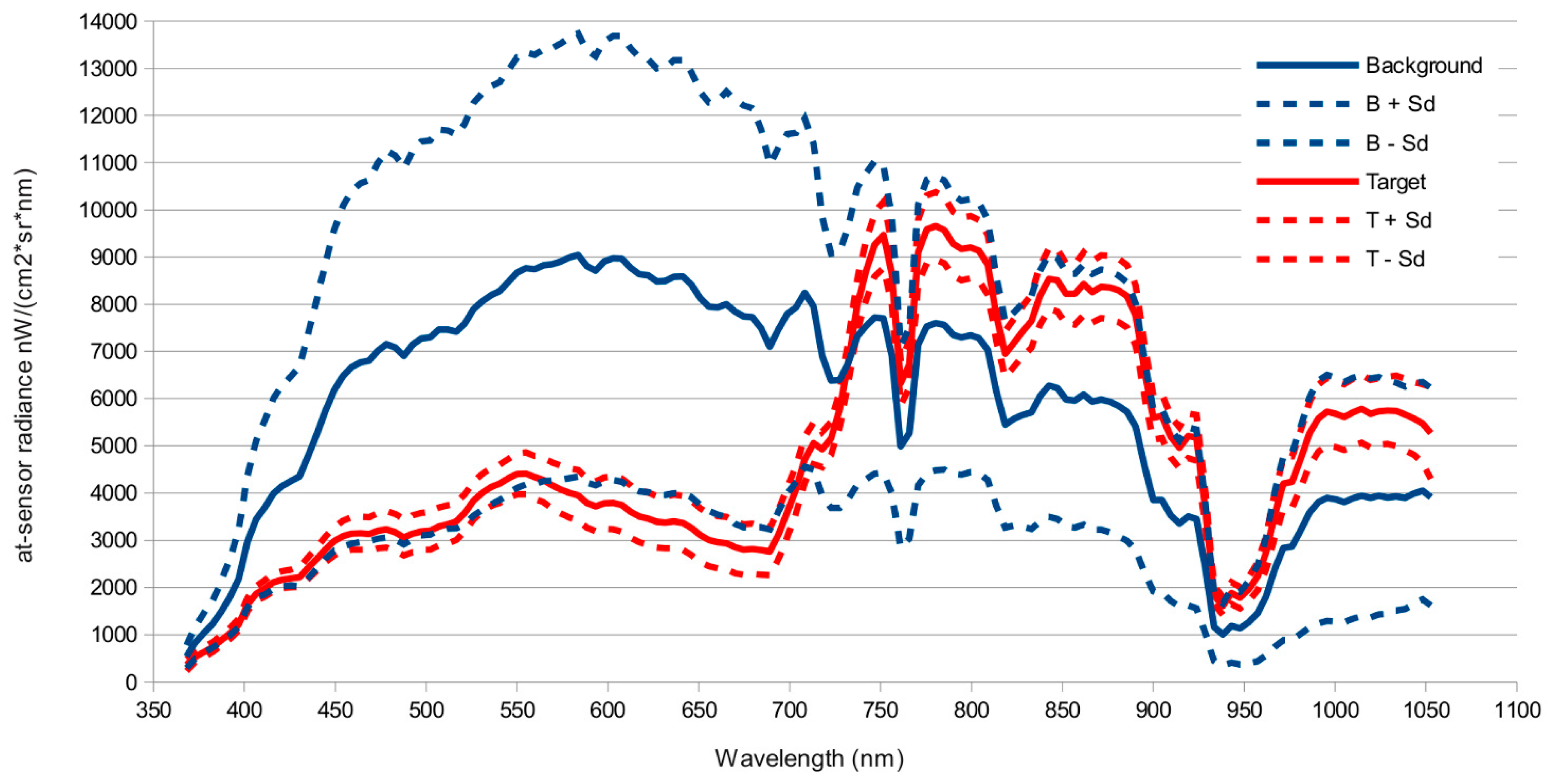
Our results show it is possible to accurately map the distribution of S. densiflora in the Guadalquivir River marshes using airborne hyperspectral sensors. 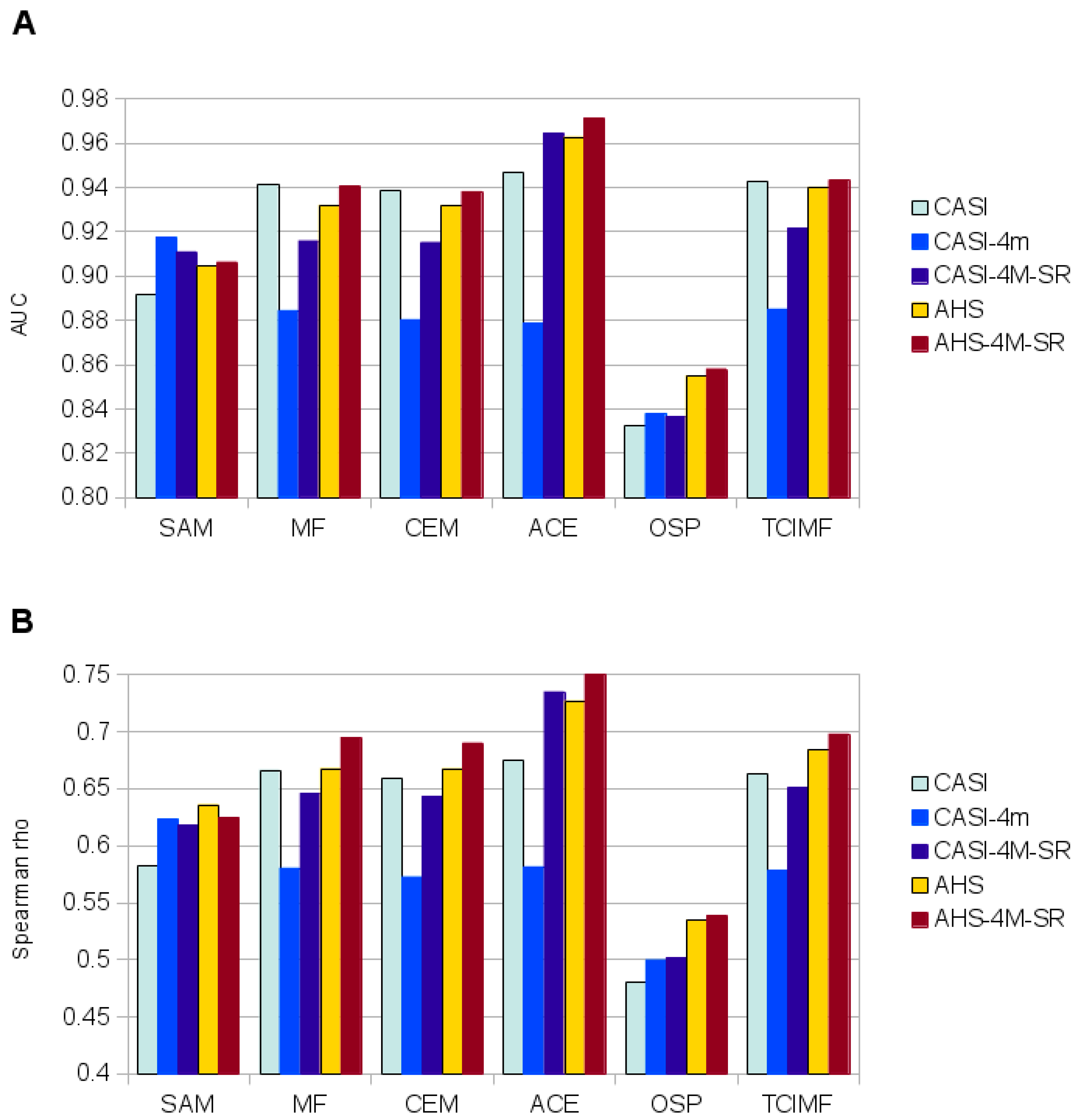The results obtained were very promising using at-sensor radiance images and radiance spectra extracted from field delineated targets, without the need of an atmospheric correction or the use of data reduction techniques like the Minimum Noise Fraction transformation [26,51]. This simplification halved computation time of detection models. Atmospheric correction and Minimum Noise Fraction Transformation only significantly improved detection for those algorithms that performed worse (SAM, OSP) on the original images, but did not improved predictions for the methods that performed best (ACE, TCIMF, MF or CEM). Both sensors tested, and most of the target detection models, gave reasonable to good results, although AHS sensor clearly outperformed CASI. The results indicated also significant effect of spatial resolution and spectral resolution. While higher spatial resolution seemed to be better, spectral resolution had the opposite effect and a reduced number of wider bands in the VNIR had a better performance than original images.

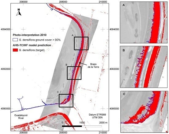
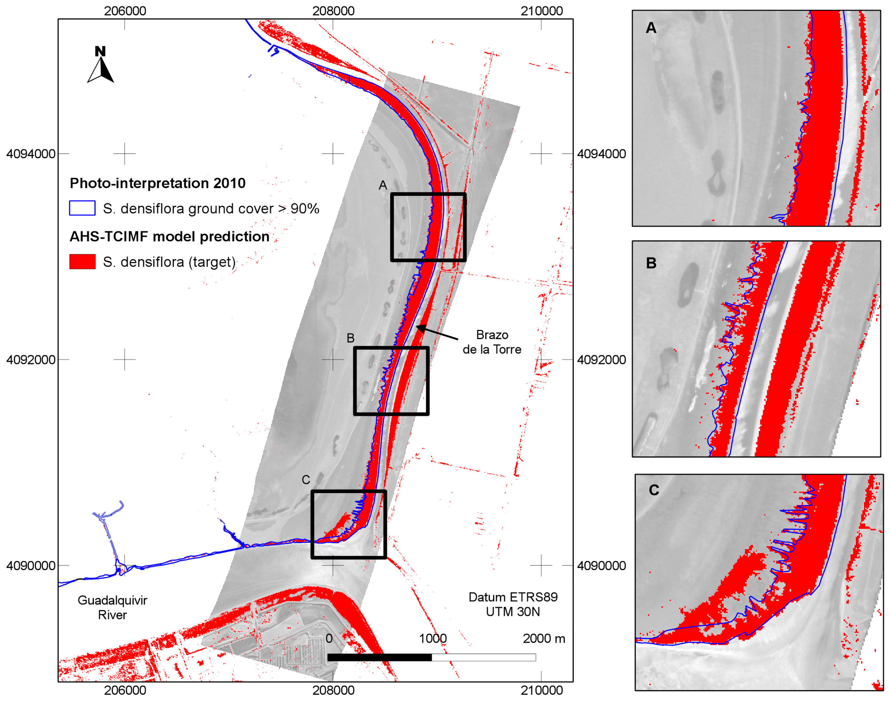
The general predictions of the spatial distribution of S. densiflora in the study area (Figure 5) tended to agree well with our previous knowledge of the species distribution, and was also in agreement with a previous photo interpretation of the study area (Figure 6). The CASI image had a higher spatial and spectral resolution in the visible range, and a higher number of spectral bands, but this did not result in a clear discrimination advantage for the target of interest. 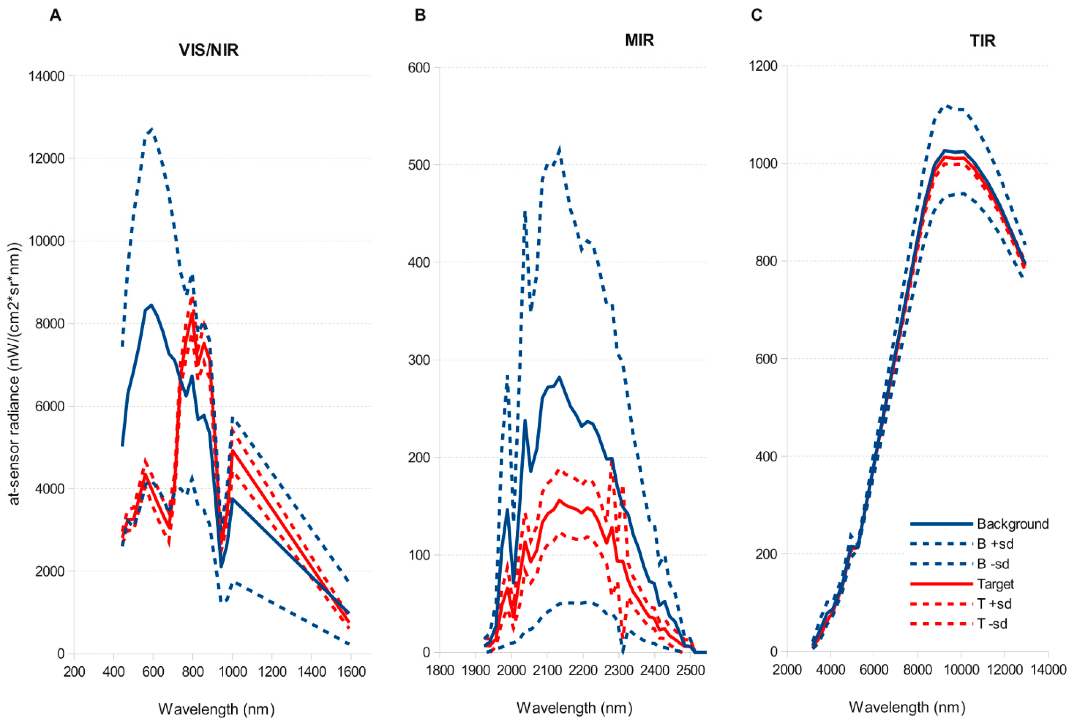The large dense monospecific stands of S. densiflora that dominate the banks of the river result in less mixed pixels so the 4 m pixel of AHS could also help in classification accuracy [66] but the decline in accuracy of CASI when resampled at 4 m suggest this is not the main factor. The AHS has a wider spectral range covering the VIS-NIR, SWIR, MIR and TIR parts of the spectrum that provides more dimensionality to discriminate target from background. This wider spectral range does not explain the better performance of AHS, because an image with the first 20 bands in the VNIR range performed slightly better than the original image with 79 bands. The better signal to noise ratio (SNR) in the AHS sensor is probably the explanation for the better performance of this sensor. The empirical mean SNR of the CASI sensor in our flight was 91.21 nW/(cm²·sr·nm), (range 4.36–184.46) versus a SNR of 246.76 (range 0.29–914.34) of the VIS-MIR channels of the AHS sensor. Detection errors caused by noise would also explain why CASI detection improves with spectral resampling. Belluco et al. [51] indicate that in marshes spatial resolution is more important than spectral resolution, but against the expectation, the higher spatial resolution of the CASI sensor did not result in an advantage when compared with the AHS. At the same time, the higher spatial resolution of the CASI image is an advantage by itself as can be seen by the reduction in performance of CASI when resampled to the coarser resolution of AHS (Table 5). This is also apparent in the GLM model (Table 6) that indicates that a higher spatial resolution improves prediction.

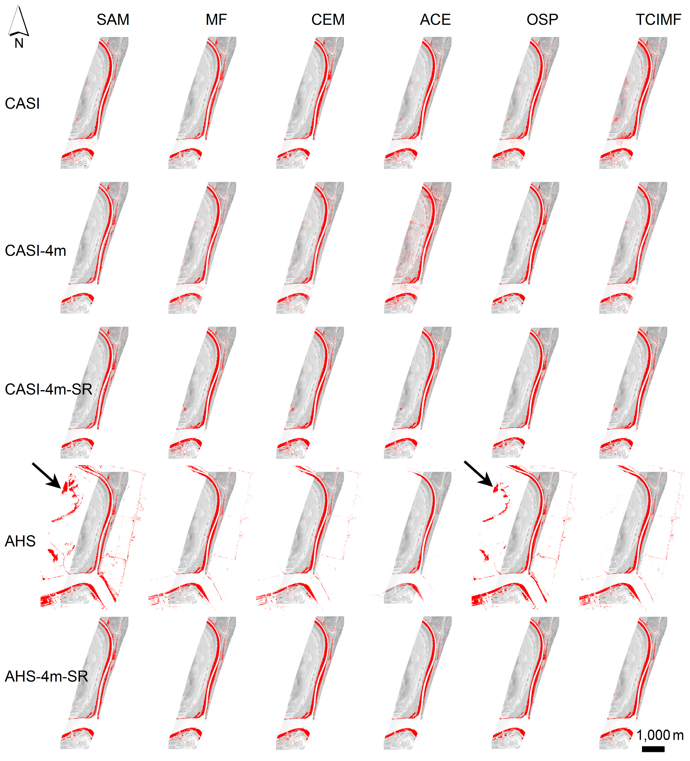
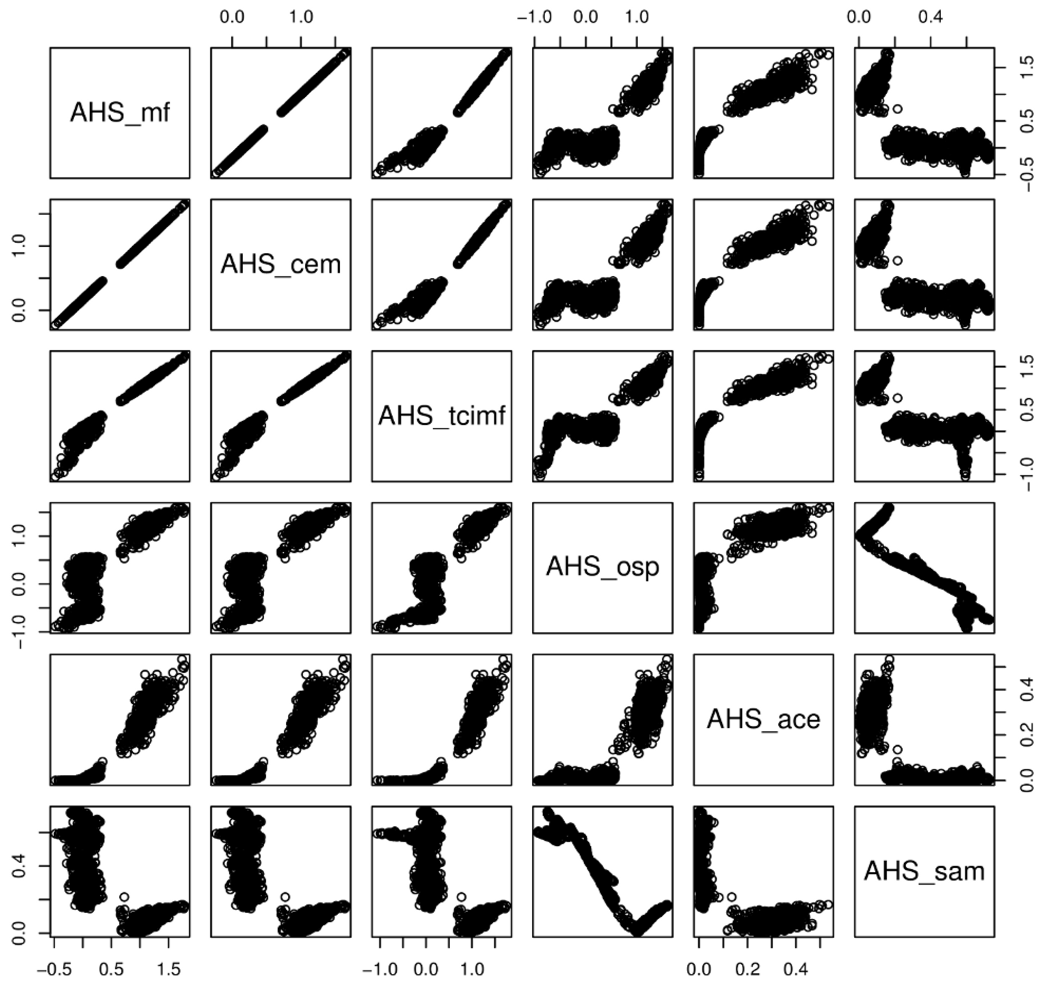
The different spectral target detection algorithms tested gave, in general, similar good results. In our case ACE outperformed the rest both with the CASI and the AHS images at the field evaluation site. This was a stronger test for the models because they were tested at a different area, target cover data were recorded in a semi-quantitative scale, evaluation points were sampled in areas where S. densiflora could grow, and models tended to differ in prediction. With the test polygons (validation) four methods (ACE, TCIMF, MF and CEM) gave a perfect discrimination on the AHS image, and almost perfect (AUC = 0.9999) on the CASI image. Three methods (TCIMF, MF and CEM) gave almost identical results for each pixel (Figure 7), suggesting that, in our setting, although algorithms differ their predictions cannot be distinguished. The OSP and the SAM algorithms were the ones that performed worse for both sensors, both with test polygons (validation) and at the new field evaluation site. They were also the ones that benefited from an atmospheric correction and MNF transformation. In addition, the classified images of OSP and SAM algorithms on the AHS image indicated the presence of S. densiflora stands in areas where the species is not present like the shores of the “Lucio de los Ansares” (Figure 5), suggesting that some models could perform poorly if extrapolated to other areas. 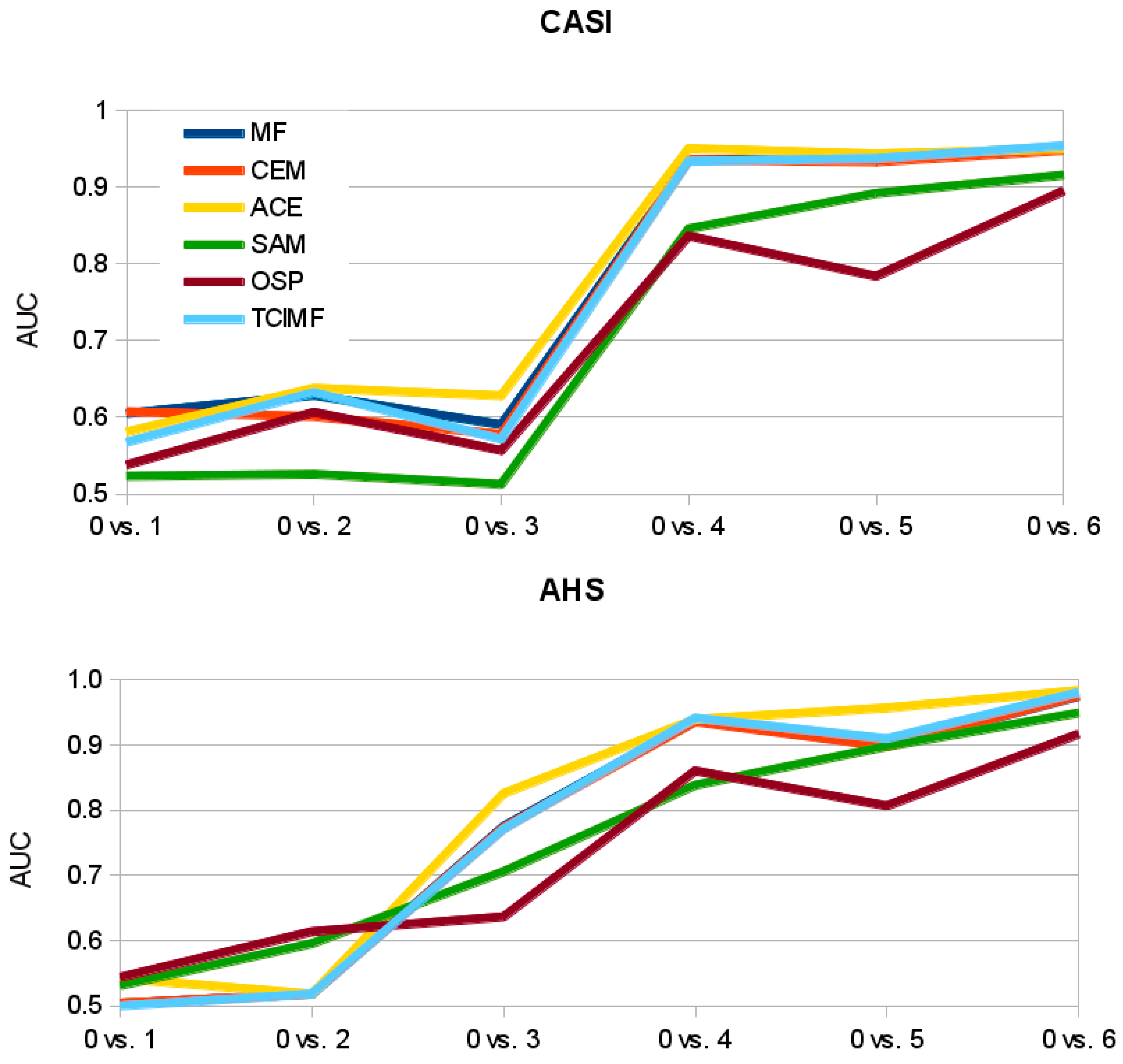However, on the other hand, the SAM algorithm showed a high correlation with S. densiflora coverage at the field evaluation site (Figure 8B) and a more gradual response in AUC values with the increase in S. densiflora ground-cover (Figure 9). Other algorithms like ACE and TCIMF show a sharper step in the increase in AUC with increase in ground-cover (Figure 9). This suggests that SAM might outperform the other algorithms when the aim is coverage estimation instead of target detection.

The high target detection accuracy showed by our results should be taken with caution, as it is based on a single date and a relatively small study site. The methods should be tested on a larger area and with a wider range of vegetation communities before using them operationally.

In this study, we have obtained a greater accuracy in the detection of S. densiflora stands than in the single previous work we know in which hyperspectral sensors have been used for the identification of the species in salt-marshes. Judd et al. [24] flew the PHILLS II hyperspectral sensor (421–966 nm, with 112 bands 4.5 nm wide) at a ground resolution of 4 m in Humboldt Bay, Northern California, obtaining a correct classification rate of 85.1% (Kappa = 0.762) for three dominant plant species (Salicornia virginica, Ditichlis spicata, and S. densiflora). For S. densiflora in this study they obtained reasonable omission errors (7.1%) but high commission errors (31.6%). Our best result with the TCIMF detection algorithm and AHS sensor has a 100% correct classification rate (Kappa = 1). If we consider our results using a hyperspectral sensor more similar to the PHILLS II, the CASI (360–1052 nm, 144 bands 2.5 nm wide), and at the same spatial resolution, 4 m, our results are still much better (omission error = 2.06%, commission error = 2.39%, Kappa = 0.965, correct classification rate = 98.38%). It is difficult to compare our results with previous work on species detection with hyperspectral sensors, because the aims of the studies, the species of interest, the habitats, the sensors used, the modeling methods, and even the way of reporting results vary greatly among studies. Previous plant classification studies with hyperspectral sensors in wetlands give correct classification rates ranging from 65% for vegetation communities in the Everglades, Florida [20], 93% for Egeria densa detection at local sites in the Sacramento-San Joaquin Delta [35] up to 99.2% for salt-marsh communities at San Felice marsh at the Lagoon of Venice, Italy [67].But at the same time, a single invasive species Colubrina asiatica gave 100% correct classification rates in the same study in the Everglades [20], and Egeria densa was poorly detected when models were extrapolated to the coarse scale of the whole Sacramento-San Joaquin Delta (29% correct classification rate) [35]. It has been shown that many factors influence plant species detection with hyperspectral sensors that are due not only to the plant species spectral characteristics and the study design but also the environmental context like species, structural and landscape diversity of the site [26]. For this reason, although our results were very good in detecting S. densiflora it still needs to be tested if our models can be extrapolated to the whole Doñana marshes with similar success.

One of the aims of our study was to test if species detection with hyperspectral sensors could be employed operationally, using methods that can be readily available for non-experts in remote sensing data analysis. Our results are encouraging because we were able to get almost 100% discrimination of S. densiflora without the need of an atmospheric correction or data reduction techniques, just working with raw band data. The models cannot be directly extrapolated to other hyperspectral sensors, other dates, or other areas flown with different atmospheric conditions. However, some of the methods are easy to employ operationally as they only require the identification of a few S. densiflora populations present in the image, information usually available to park managers, to extract a few training spectra. These methods could be tested in hyperspectral satellite images (Chris PROBA, Hyperion) as this would facilitate and reduce costs of regular monitoring of S. densiflora distribution. All the spectral detection methods employed are implemented in the “Target Detection Wizard” in ENVI [39], so they can be used with little training by a technician. Our results also indicate that AHS is a hyperspectral sensor that, although has a limited spectral resolution in the visible and near infrared and has received limited attention for vegetation mapping [38,57], can be successfully used for plant species discrimination. Our results also indicate that spectral detection techniques deriving from statistical signal processing like CEM, ACE, OSP and TCIMF [53] that have received limited attention in the literature of vegetation classification with remote sensing are methods that can give similar or better results to those currently employed like SAM.

6. Conclusions

The target S. densiflora was easy to detect in the marshes by all algorithms in images of both sensors. The best methods (adaptive coherence estimator and target-constrained interference minimized filter) on the best sensor (AHS) produced 100% discrimination (Kappa = 1, AUC = 1) at the study site and only some decline in performance when extrapolated to a new area (Kappa = 0.7, AUC = 0.94). AHS outperformed CASI in spite of having a coarser spatial resolution (4-m vs. 1-m) and lower spectral resolution in the visible and near-infrared range probably due to its better signal to noise ratio. Our conclusions are that it is possible to use hyperspectral sensors to map the early spread of S. densiflora in the Guadalquivir River marshes. AHS is the best hyperspectral sensor for this task and the signal processing techniques target-constrained interference minimized filter and adaptive coherence estimator are the target detection that worked the best in our particular setting. They are techniques that could be employed operationally by park technicians with limited remote sensing expertise using a simplified processing protocol with hyperspectral images.

References

1. Bortolus, A. The austral cordgrass Spartina densiflora Brong.: Its taxonomy, biogeography and natural history. J. Biogeogr. 2005, 33, 158–168. [Google Scholar] [CrossRef]
2. Castillo, J.M.; Fernández-Baco, L.; Castellanos, E.M.; Luque, C.J.; Figueroa, M.E.; Davy, A.J. Lower limits of Spartina densiflora and S. maritima in a Mediterranean salt marsh determined by different ecophysiological tolerances. J. Ecol. 2000, 88, 801–812. [Google Scholar] [CrossRef]
3. Figueroa, M.E.; Castellanos, E.M. Vertical structure of Spartina maritima and Spartina densiflora in Mediterranean marshes. In Plant Form and Vegetation Structure; Werger, M.J.A., van der Aart, P.J., During, H.J., Verhoeven, J.T.A., Eds.; SPB Academic Publishing: The Hague, The Netherlands, 1988; pp. 105–108. [Google Scholar]
4. Peixoto, A.R.; Costa, C.S.B. Produção primária líquida aérea de Spartina densiflora Brong. (Poaceae) no estuário da laguna dos Patos, Rio Grande do Sul, Brasil. Iheringia Sér. Bot. 2004, 59, 27–34. [Google Scholar]
5. González Trilla, G.; De Marco, S.; Marcovecchio, J.; Vicari, R.; Kandus, P. Net primary productivity of Spartina densiflora brong in an SW Atlantic Coastal salt marsh. Estuar. Coast. 2010, 33, 953–962. [Google Scholar] [CrossRef]
6. Gallego Fernández, J.B.; García Novo, F. High-intensity versus low-intensity restoration alternatives of a tidal marsh in Guadalquivir estuary, SW Spain. Ecol. Eng. 2007, 30, 112–121. [Google Scholar] [CrossRef]
7. Simberloff, D. How much information on population biology is needed to manage introduced species? Conserv. Biol. 2003, 17, 83–92. [Google Scholar] [CrossRef]
8. Rejmánek, M.; Pitcairn, M.J. When is eradication of exotic pest plants a realistic goal. In Turning the Tide: the Eradication of Invasive Species: Proceedings of the International Conference on Eradication of Island Invasives; Veitch, C.R., Clout, M.N., Eds.; IUCN: Cambridge, UK, 2002; pp. 249–253. [Google Scholar]
9. Mateos-Naranjo, E.; Redondo-Gómez, S.; Luque, C.J.; Castellanos, E.M.; Davy, A.J.; Figueroa, M.E. Environmental limitations on recruitment from seed in invasive Spartina densiflora on a southern European salt marsh. Estuar. Coast. Shelf Sci. 2008, 79, 727–732. [Google Scholar] [CrossRef]
10. Hestir, E.L.; Khanna, S.; Andrew, M.E.; Santos, M.J.; Viers, J.H.; Greenberg, J.A.; Rajapakse, S.S.; Ustin, S.L. Identification of invasive vegetation using hyperspectral remote sensing in the California Delta ecosystem. Remote Sens. Environ. 2008, 112, 4034–4047. [Google Scholar] [CrossRef]
11. He, K.S.; Rocchini, D.; Neteler, M.; Nagendra, H. Benefits of hyperspectral remote sensing for tracking plant invasions. Divers. Distrib. 2011, 17, 381–392. [Google Scholar] [CrossRef]
12. Joshi, C.; de Leeuw, J.; van Duren, I.C. Remote sensing and GIS applications for mapping and spatial modelling of invasive species. In Proceedings of the ISPRS Congress, Istanbul, Turkey, 12–23 July 2004.
13. Cochrane, M.A. Using vegetation reflectance variability for species level classification of hyperspectral data. Int. J. Remote Sens. 2000, 21, 2075–2087. [Google Scholar] [CrossRef]
14. Evangelista, P.H.; Stohlgren, T.J.; Morisette, J.T.; Kumar, S. Mapping invasive Tamarisk (Tamarix): A comparison of single-scene and time-series analyses of remotely sensed data. Remote Sens. 2009, 1, 519–533. [Google Scholar] [CrossRef]
15. Scharlemann, J.P.W.; Benz, D.; Hay, S.I.; Purse, B.V.; Tatem, A.J.; Wint, G.R.W.; Rogers, D.J. Global data for ecology and epidemiology: A novel algorithm for temporal Fourier processing MODIS data. PLoS ONE 2008. [Google Scholar] [CrossRef] [PubMed]
16. Díaz-Delgado, R.; Aragonés, D.; Ameztoy, I.; Bustamante, J. Monitoring marsh dynamics through remote sensing. In Conservation Monitoring in Freshwater Habitats; Hurford, C., Scheneider, M., Cowx, I., Eds.; Springer: Berlin, Germany, 2010; pp. 375–386. [Google Scholar]
17. Asner, G.P.; Jones, M.O.; Martin, R.E.; Knapp, D.E.; Hughes, R.F. Remote sensing of native and invasive species in Hawaiian forests. Remote Sens. Environ. 2008, 112, 1912–1926. [Google Scholar] [CrossRef]
18. Laba, M.; Blair, B.; Downs, R.; Monger, B.; Philpot, W.; Smith, S.; Sullivan, P.; Baveye, P.C. Use of textural measurements to map invasive wetland plants in the Hudson River National Estuarine Research Reserve with IKONOS satellite imagery. Remote Sens. Environ. 2010, 114, 876–886. [Google Scholar] [CrossRef]
19. Parker Williams, A.; Hunt, E.R. Estimation of leafy spurge cover from hyperspectral imagery using mixture tuned matched filtering. Remote Sens. Environ. 2002, 82, 446–456. [Google Scholar] [CrossRef]
20. Hirano, A.; Madden, M.; Welch, R. Hyperspectral image data for mapping wetland vegetation. Wetlands 2003, 23, 436–448. [Google Scholar] [CrossRef]
21. Lass, L.; Thill, D.; Shafii, B.; Prather, T. Detecting spotted knapweed (Centaurea maculosa) with hyperspectral remote sensing technology. Weed Technol. 2002, 16, 426–432. [Google Scholar] [CrossRef]
22. Lawrence, R.L.; Wood, S.D.; Sheley, R.L. Mapping invasive plants using hyperspectral imagery and Breiman Cutler classifications (randomForest). Remote Sens. Environ. 2006, 100, 356–362. [Google Scholar] [CrossRef]
23. Hamada, Y.; Stow, D.A.; Coulter, L.L.; Jafolla, J.C.; Hendricks, L.W. Detecting Tamarisk species (Tamarix spp.) in riparian habitats of Southern California using high spatial resolution hyperspectral imagery. Remote Sens. Environ. 2007, 109, 237–248. [Google Scholar] [CrossRef]
24. Judd, C.; Steinberg, S.; Shaughnessy, F.; Crawford, G. Mapping salt marsh vegetation using aerial hyperspectral imagery and linear unmixing in Humboldt Bay, California. Wetlands 2007, 27, 1144–1152. [Google Scholar] [CrossRef]
25. Pengra, B.W.; Johnston, C.A.; Loveland, T.R. Mapping an invasive plant, Phragmites australis, in coastal wetlands using the EO-1 Hyperion hyperspectral sensor. Remote Sens. Environ. 2007, 108, 74–81. [Google Scholar] [CrossRef]
26. Andrew, M.E.; Ustin, S.L. The role of environmental context in mapping invasive plants with hyperspectral image data. Remote Sens. Environ. 2008, 112, 4301–4317. [Google Scholar] [CrossRef]
27. Carter, G.A.; Lucas, K.L.; Blossom, G.A.; Lassitter, C.L.; Holiday, D.M.; Mooneyhan, D.S.; Fastring, D.R.; Holcombe, T.R.; Griffith, J.A. Remote sensing and mapping of Tamarisk along the Colorado River, USA: A comparative use of summer-acquired Hyperion, Thematic Mapper and QuickBird data. Remote Sens. 2009, 1, 318–329. [Google Scholar] [CrossRef]
28. Mitchell, J.J.; Glenn, N.F. Subpixel abundance estimates in mixture-tuned matched filtering classifications of leafy spurge (Euphorbia esula L.). Int. J. Remote Sens. 2009, 30, 6099–6119. [Google Scholar] [CrossRef]
29. Demuro, M.; Chisholm, L. Assessment of Hyperion for characterizing mangrove communities. In Proceedings of the 12th JPL AVIRIS Airborne Earth Science Workshop, Pasadena, CA, USA, 31 March 2003.
30. Ozesmi, S.L.; Bauer, M.E. Satellite remote sensing of wetlands. Wetl. Ecol. Manag. 2002, 10, 381–402. [Google Scholar] [CrossRef]
31. Miao, X.; Gong, P.; Swope, S.; Pu, R.; Carruthers, R.; Anderson, G.L.; Heaton, J.S.; Tracy, C.R. Estimation of yellow starthistle abundance through CASI-2 hyperspectral imagery using linear spectral mixture models. Remote Sens. Environ. 2006, 101, 329–341. [Google Scholar] [CrossRef]
32. Root, R.; Zarco-Tejada, P.; Pinilla, C. Identification, Classification, and Mapping of Invasive Leafy Spurge using Hyperion, AVIRIS, and CASI; Earth Observing-1 Preliminary Technology and Science Validation Report, Part 3. Available online: https://eo1.gsfc.nasa.gov/new/validationReport/Technology/Documents/Tech.Val.Report/Science_Summary_Root.pdf (accessed on 30 November 2016).
33. Pu, R.; Gong, P.; Tian, Y.; Miao, X.; Carruthers, R.I.; Anderson, G.L. Invasive species change detection using artificial neural networks and CASI hyperspectral imagery. Environ. Monit. Assess. 2008, 140, 15–32. [Google Scholar] [CrossRef] [PubMed]
34. Anderson, G.L.; Carruthers, R.I.; Ge, S.; Gong, P. Monitoring of invasive Tamarix distribution and effects of biological control with airborne hyperspectral remote sensing. Int. J. Remote Sens. 2005, 26, 2487–2489. [Google Scholar] [CrossRef]
35. Underwood, E.C.; Mulitsch, M.J.; Greenberg, J.A.; Whiting, M.L.; Ustin, S.L.; Kefauver, S.C. Mapping invasive aquatic vegetation in the Sacramento-San Joaquin Delta using hyperspectral imagery. Environ. Monit. Assess. 2006, 121, 47–64. [Google Scholar] [CrossRef] [PubMed]
36. Lass, L.W.; Prather, T.S.; Glenn, N.F.; Weber, K.T.; Mundt, J.T.; Pettingill, J. A review of remote sensing of invasive weeds and example of the early detection of spotted knapweed (Centaurea maculosa) and babysbreath (Gypsophila paniculata) with a hyperspectral sensor. Weed Sci. 2005, 53, 242–251. [Google Scholar] [CrossRef]
37. Theriault, C.; Scheibling, R.; Hatcher, B.; Jones, W. Mapping the distribution of an invasive marine alga (Codium fragile spp. tomentosoides) in optically shallow coastal waters using the compact airborne spectrographic imager (CASI). Can. J. Remote Sens. 2006, 32, 315–329. [Google Scholar]
38. Jiménez Michavilla, M. Cartografía de especies de matorral de la Reserva Biológica de Doñana mediante el sistema hyperespectral aeroportado INTA-AHS. Implicaciones en el estudio y seguimiento del matorral de Doñana. Ph.D. Thesis, Universidad Autónoma de Madrid, Madrid, Spain, 2011. [Google Scholar]
39. Exelis Visual Information Solutions. ENVI User’s Guide: ENVI Version 4.6.1, Exelis Visual Information Solutions: Boulder, CO, USA, 2010.
40. Espinar, J.L.; García, L.V.; Clemente, L. Seed storage conditions change the germination pattern of clonal growth plants in Mediterranean salt marshes. Am. J. Bot. 2005, 92, 1094–1101. [Google Scholar] [CrossRef] [PubMed]
41. García Murillo, P.; Fernández Zamudio, R.; Cirujano, S.; Sousa, A. Aquatic macrophytes in Donana protected area (SW Spain): An overview. Limnetica 2006, 25, 71–80. [Google Scholar]
42. Rivas-Martínez, S.; Costa Talens, M.; Castroviejo, S.; Valdés, E. Vegetación de Doñana (Huelva, España). Lazaroa 1980, 2, 5–189. [Google Scholar]
43. Rejas, J.G.; Prado, E.; Jiménez, M.; Fernández-Renau, A.; Gómez, J.A.; de Miguel, E. Caracterización del sensor Hiperespectral AHS para la georreferenciación directa de imágenes a partir de un sistema inercial GPS/IMU. In Proceedings of the 6a Semana de Geomática, Barcelona, Spain, 8–13 August 2005.
44. Solís, R.; Aragonés, D.; Bustamante, J. Evaluación de la precisión de georeferenciación de imágenes aeroportadas del sensor hiperespectral AHS sobre Doñana. In Teledetección: Agua y desarrollo sostenible. XIII Congreso de la Asociación Española de Teledetección; Montesinos, S., Fernández, L., Eds.; Geosys: Calatayud, Spain, 2009; pp. 437–440. [Google Scholar]
45. Bernstein, L.S.; Adler-Golden, S.M.; Sundberg, R.L.; Levine, R.Y.; Perkins, T.C.; Berk, A.; Ratkowski, A.J.; Felde, G.; Hoke, M.L. Validation of the QUick atmospheric correction (QUAC) algorithm for VNIR-SWIR multi- and hyperspectral imagery. Proc. SPIE 2005. [Google Scholar] [CrossRef]
46. Bernstein, L.S.; Adler-Golden, S.M.; Sundberg, R.L.; Ratkowski, A.J. Improved reflectance retrieval from hyper and multispectral imagery without prior scene or sensor information. Proc. SPIE 2006. [Google Scholar] [CrossRef]
47. Matthew, M.W.; Adler-Golden, S.M.; Berk, A.; Richtsmeier, S.C.; Levine, R.Y.; Bernstein, L.S.; Acharya, P.K.; Anderson, G.P.; Felde, G.W.; Hoke, M.L.; et al. Status of atmospheric correction using a MODTRAN4-based algorithm. Proc. SPIE 2000. [Google Scholar] [CrossRef]
48. Smith, G.M.; Milton, E.J. The use of the empirical line method to calibrate remotely sensed data to reflectance. Int. J. Remote Sens. 1999, 20, 2653–2662. [Google Scholar] [CrossRef]
49. Fernández-Renau, A.; Gómez, J.A.; de Miguel, E. The INTA AHS system. Proc. SPIE 2005. [Google Scholar] [CrossRef]
50. Young, S.J.; Johnson, B.R.; Hackwell, J.A. An in-scene method for atmospheric compensation of thermal hyperspectral data. J. Geophys. Res. Atmos. 2002. [Google Scholar] [CrossRef]
51. Green, A.A.; Berman, M.; Switzer, P.; Craig, M.D. A transformation for ordering multispectral data in terms of image quality with implications for noise removal. IEEE Trans. Geosci. Remote Sens. 1988, 26, 65–74. [Google Scholar] [CrossRef]
52. Youngentob, K.N.; Roberts, D.A.; Held, A.A.; Dennison, P.E.; Jia, X.; Lindenmayer, D.B. Mapping two Eucalyptus subgenera using multiple endmember spectral mixture analysis and continuum-removed imaging spectrometry data. Remote Sens. Environ. 2011, 115, 1115–1128. [Google Scholar] [CrossRef]
53. Chang, C.I. Hyperspectral Imaging: Techniques for Spectral Detection and Classification; Kluwer Academic Publishers: New York, NY, USA, 2003. [Google Scholar]
54. Marcum, J.I. A Statistical Theory of Target Detection by Pulsed Radar; U.S. Force Project Rand Research Memorandum: Santa Monica, CA, USA, 1947. [Google Scholar]
55. Kacur, J.; Rozinaj, G.; Herrera-Garcia, S. Speech signal detection in a noisy environment using neural networks and cepstral matrices. J. Electr. Eng. 2004, 55, 131–137. [Google Scholar]
56. Kamal, M.; Phinn, S. Hyperspectral data for mangrove species mapping: A comparison of pixel-based and object-based approach. Remote Sens. 2011, 3, 2222–2242. [Google Scholar] [CrossRef]
57. Casal, G.; Sanchez-Carnero, N.; Dominguez-Gomez, J.A.; Kutser, T.; Freire, J. Assessment of AHS (Airborne Hyperspectral Scanner) sensor to map macroalgal communities on the Ria de vigo and Ria de Aldan coast (NW Spain). Mar. Biol. 2012, 159, 1997–2013. [Google Scholar] [CrossRef]
58. Buddenbaum, H.; Schlerf, M.; Hill, J. Classification of coniferous tree species and age classes using hyperspectral data and geostatistical methods. Int. J. Remote Sens. 2005, 26, 5453–5465. [Google Scholar] [CrossRef]
59. Bertels, L.; Deronde, B.; Kempeneers, S.; Tortelboom, E. Potentials of airborne hyperspectral remote sensing for vegetation mapping of spatially heterogeneous dynamic dunes, a case study along the Belgian coastline. In Proceedings of the Dunes and Estuaries 2005: International Conference on Nature Restoration Practices in European Coastal Habitats, Koksijde, Belgium, 19–23 September 2005.
60. Yuhas, R.H.; Goetz, A.F.H.; Boardman, J.W. Discrimination among semi-arid landscape endmembers using the spectral angle mapper (SAM) algorithm. In Proceedings of the Summaries of the Third Annual JPL Airborne Geoscience Workshop, Pasadena, CA, USA, 1–5 June 1992.
61. Harsanyi, J.C. Detection and Classification of Subpixel Spectral Signatures in Hyperspectral Image Sequences. Ph.D. Thesis, University of Maryland, Baltimore County, MD, USA, 1993. [Google Scholar]
62. Harsanyi, J.C.; Farrand, W.H.; Chang, C.I. Detection and classification of subpixel signatures in hyperspectral image sequences. In Proceedings of the 1994 ASPRS Annual Conference, Reno, NV, USA, 25–28 April 1994; pp. 236–247.
63. Kraut, S.; Scharf, L.L.; Butler, R.W. The adaptive coherence estimator: A uniformly most-powerful-invariant adaptive detection statistic. IEEE Trans. Signal Process. 2005, 53, 427–438. [Google Scholar] [CrossRef]
64. Harsanyi, J.C.; Chang, C.I. Hyperspectral image classification and dimensionality reduction: An orthogonal subspace projection approach. IEEE Trans. Geosci. Remote Sens. 1994, 32, 779–785. [Google Scholar] [CrossRef]
65. R Development Core Team. R: A Language and Environment for Statistical Computing; R Foundation for Statistical Computing: Vienna, Austria, 2013. [Google Scholar]
66. Woodcock, C.E.; Strahler, A.H. The factor of scale in remote sensing. Remote Sens. Environ. 1987, 21, 311–332. [Google Scholar] [CrossRef]
67. Belluco, E.; Camuffo, M.; Ferrari, S.; Modenese, L.; Silvestri, S.; Marani, A.; Marani, M. Mapping salt-marsh vegetation by multispectral and hyperspectral remote sensing. Remote Sens. Environ. 2006, 105, 54–67. [Google Scholar] [CrossRef]
Figure 1. (A) Location of Doñana National Park in southwestern Spain. (B) Location of the airborne campaign on the eastern side of Doñana marshes. Background Landsat TM image of 25 February 2011. (C) Extent of the study area (763 ha) is delimited by the false color composite of the CASI-1500 image (RGB = 861.6, 650.8, 550.1 nm) overlaid on top of the AHS image (background). (D) Zoom to an example of a few target (Spartina densiflora) (red) and background (white) polygons overlaid on the CASI image. Solid polygons correspond to training sites and hollow polygons to test sites used for model validation. (E) Location of sampling points at the evaluation site of “Codo de la Esparraguera” overlaid on the CASI image. Map projections: ETRS89/UTM Zone 30 N. Map grids: (A) and (B) in decimal degrees, (C) UTM in m.
Remotesensing 08 01001 g001
Figure 2. Mean ± s.d. of target and background radiance spectra as extracted from the CASI image.
Remotesensing 08 01001 g002
Figure 3. Mean ± s.d. of target and background radiance spectra as extracted from the AHS image. (A) Visible and near-infrared. (B) Short-wave infrared. (C) Thermal infrared.
Remotesensing 08 01001 g003
Figure 4. Graphical example on how a new cut-point is estimated from rule-image values extracted with training polygons. The lower confidence limit (LCL = μ − 1.96σ) and upper confidence limit (UCL = μ + 1.96σ) of the background and target distributions are estimated. The new cut-point is (UCLbackground + LCLtarget)/2, provided that target μ > background μ. (A) represent a the situation when distributions do not overlap; and (B) a situation when they overlap.
Remotesensing 08 01001 g004
Figure 5. Predicted distribution of Spartina densiflora according to each model. S. densiflora prediction in red. Detection algorithms (in columns): Spectral Angle Mapper (SAM), Matched Filter (MF), Constrained Energy Minimization (CEM), Adaptive Coherence Estimator (ACE), Orthogonal Subspace Projection (OSP) and Target-Constrained Interference-Minimized Filter (TCIMF), and hyperspectral image (in rows) CASI, CASI-4m, CASI-4m-SR, AHS, and AHS-4m-SR. The gray background represents the study area defined by the overlap of the footprints of the CASI and AHS sensors. Black arrows represent known prediction errors by SAM and OSP at “Lucio de los Ansares” shores where we know S. densiflora is not present.
Remotesensing 08 01001 g005
Figure 6. Qualitative validation of best model prediction using a previous photo-interpretation of Spartina densiflora (blue line) on top of model prediction (in red). Model prediction according to the Target-Constrained Interference-Minimized Filter (TCIMF) algorithm on the AHS sensor image (one of the best models according to AUC). The gray background represents the area of overlap of the CASI and AHS images. Polygons overlaid in blue represent the limits of a photo-interpreted coverage of S. densiflora on the right bank of the “Brazo de la Torre” and Guadalquivir River using summer 2010 aerial photos. (AC) show details of the agreement in the limits of both data sets. (C) shows a clear disagreement that can be either an error of photo-interpretation or an error of the model. Note that the left bank, when S. densiflora is also present, was not photo-interpreted.
Remotesensing 08 01001 g006
Figure 7. Bivariate scatter plots of rule-image values for each detection algorithm in the AHS image. SAM = Spectral Angle Mapper, MF = Matched Filter, CEM = Constrained Energy Minimization, ACE = Adaptive Coherence Estimator, OSP = Orthogonal Subspace Projection, TCIMF = Target-Constrained Interference-Minimized Filter.
Remotesensing 08 01001 g007
Figure 8. Evaluation of detection algorithms. SAM = Spectral Angle Mapper, MF = Matched Filter, CEM = Constrained Energy Minimization, ACE = Adaptive Coherence Estimator, OSP = Orthogonal Subspace Projection, TCIMF = Target-Constrained Interference-Minimized Filter. Hyperspectral images: CASI-4m, CASI-4M-SR, CASI, AHS-4M-SR and AHS. Evaluation at the new site “Codo de la Esparraguera”, (A) AUC of a ROC plot for S. densiflora presence/absence at sampling points (n = 43 vs. 68). (B) Spearman Rho correlation between rule-image value and S. densiflora ground-cover class, n = 129 sample points.
Remotesensing 08 01001 g008
Figure 9. Comparative performance of algorithms to discriminate among S. densiflora ground-cover classes. Discrimination performance of each detection algorithm for CASI and AHS original images at the field validation site of “Codo de la Esparraguera”. SAM = Spectral Angle Mapper, MF = Matched Filter, CEM = Constrained Energy Minimization, ACE = Adaptive Coherence Estimator, OSP = Orthogonal Subspace Projection, TCIMF = Target-Constrained Interference-Minimized Filter. Sensors: CASI and AHS. The value in the graph indicates the AUC of a ROC plot to discriminate between the Class “0” of S. densiflora ground-cover and the remaining classes. Ground-cover classes: 0 = absence, 1 = presence < 5% cover, 2 = 5%–25%, 3 = 25%–50%, 4 = 50%–75%, 5 = 75%–99%, 6 = 100%. Sample sizes are 68, 7, 4, 7, 8, 20 and 15 respectively.
Remotesensing 08 01001 g009