
Dryland Vegetation Functional Response to Altered Rainfall Amounts and Variability Derived from Satellite Time Series Data


Abstract
:
1. Introduction
2. Materials and Methods
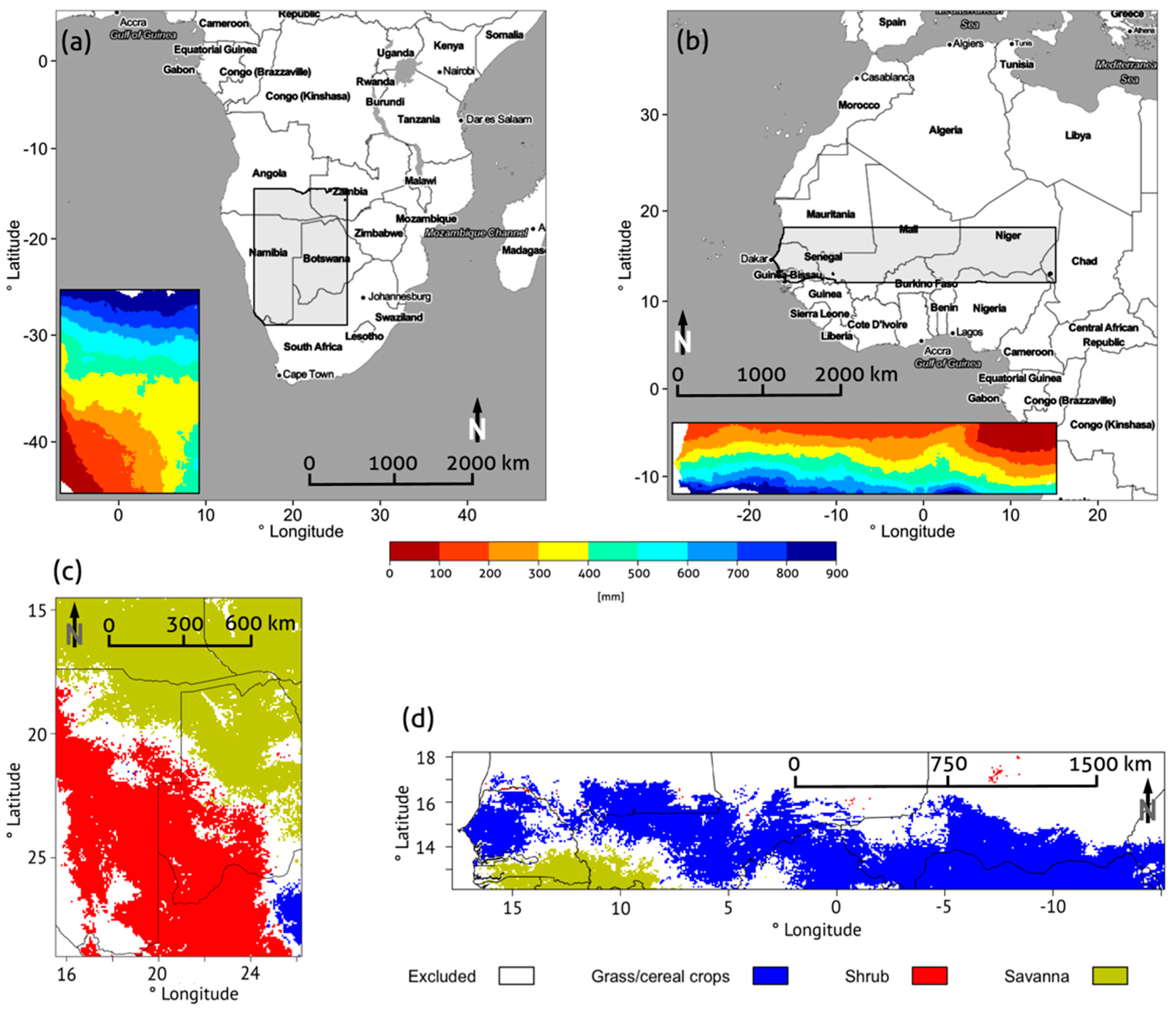
2.1. Study Regions
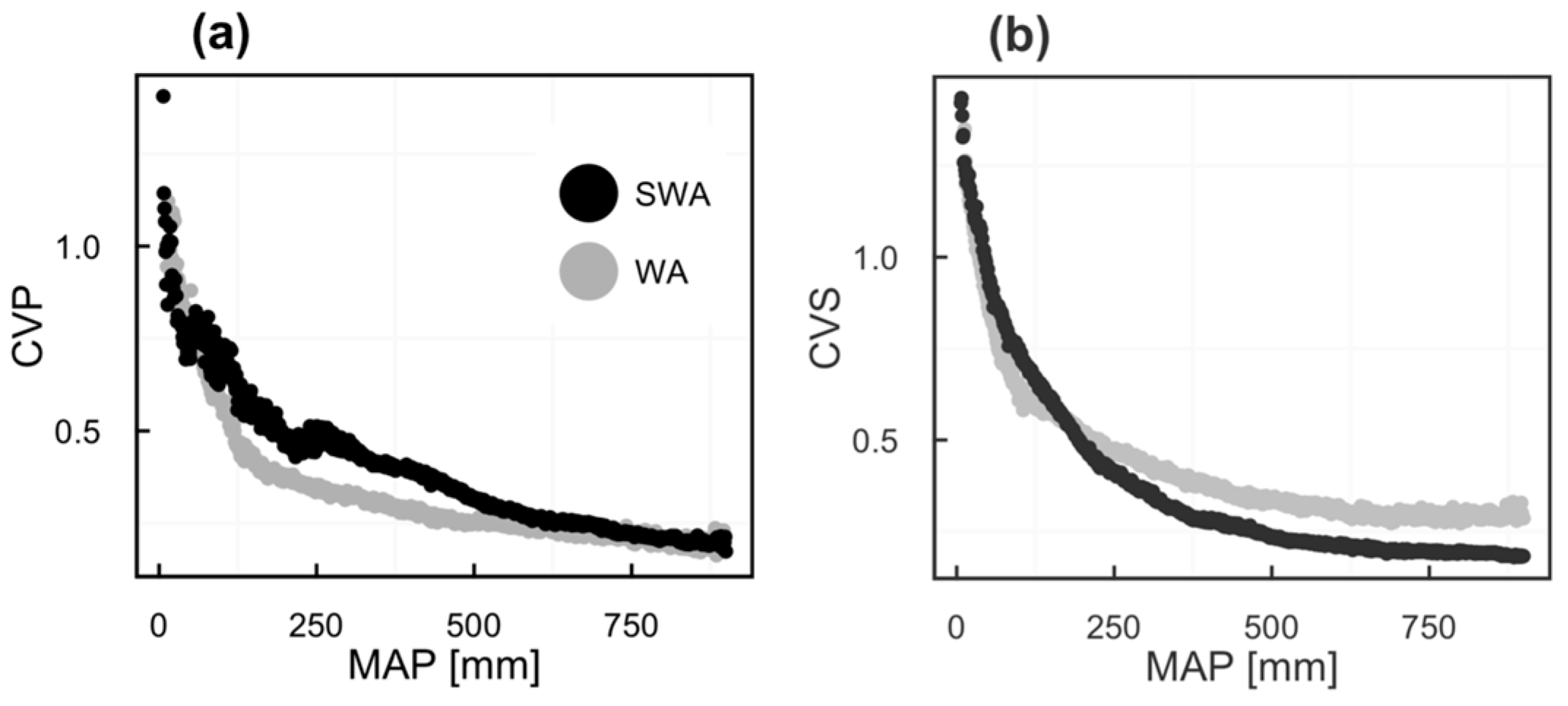
2.2. Vegetation Productivity Proxies
2.3. Rainfall Data
2.4. Land Cover Data
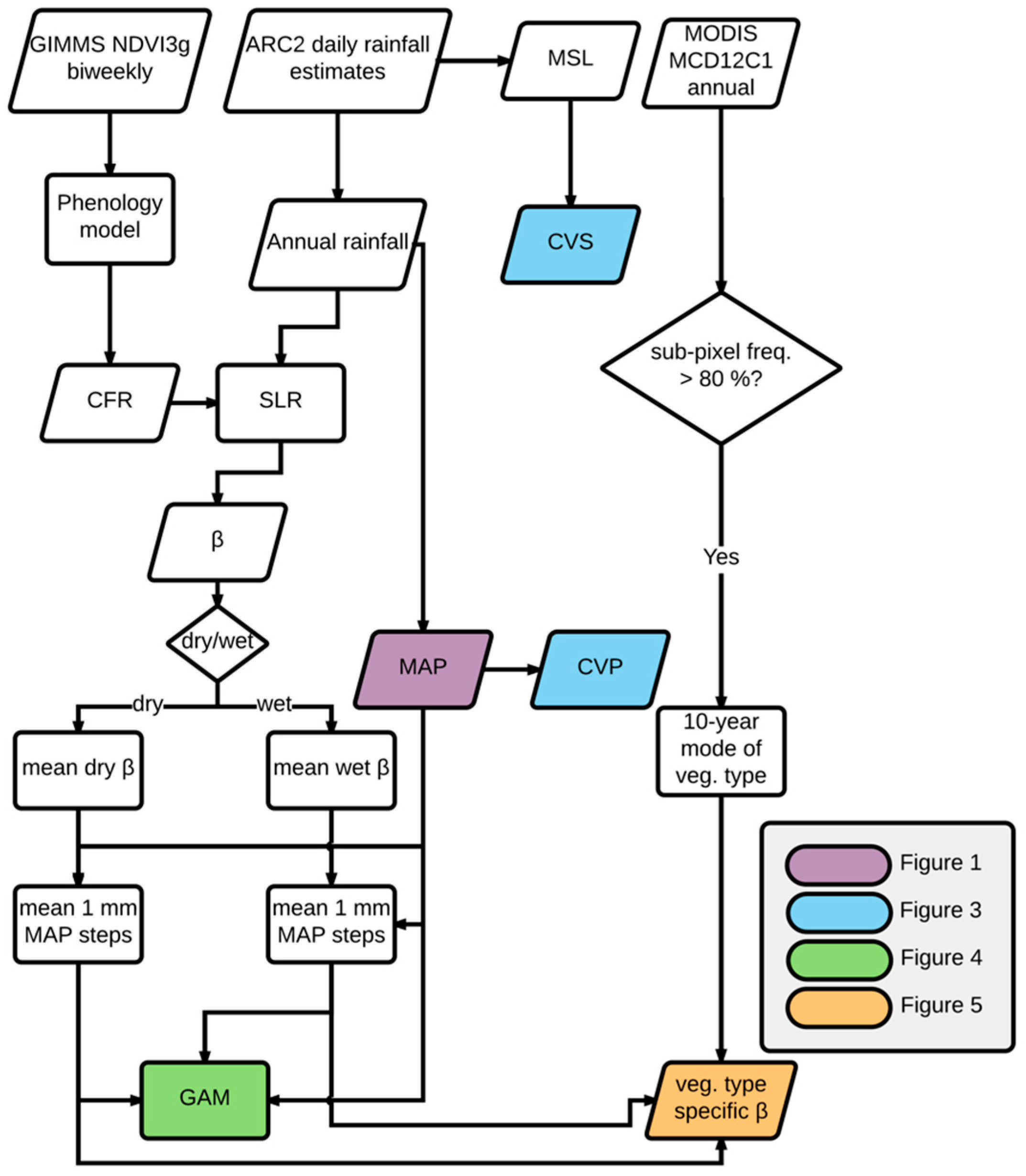
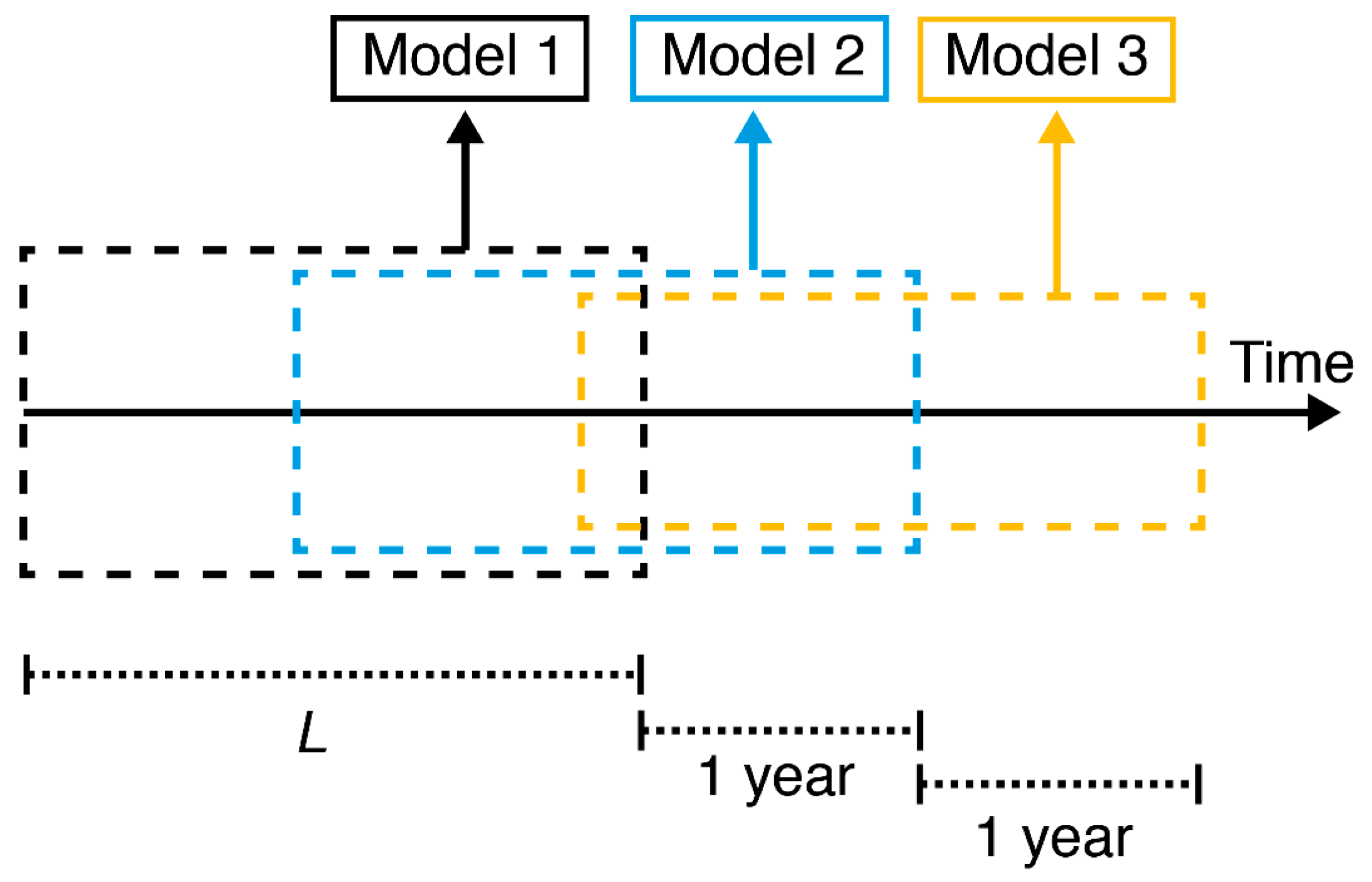
2.5. Shifting Linear Regression Models
2.6. Spatial Analysis
3. Results
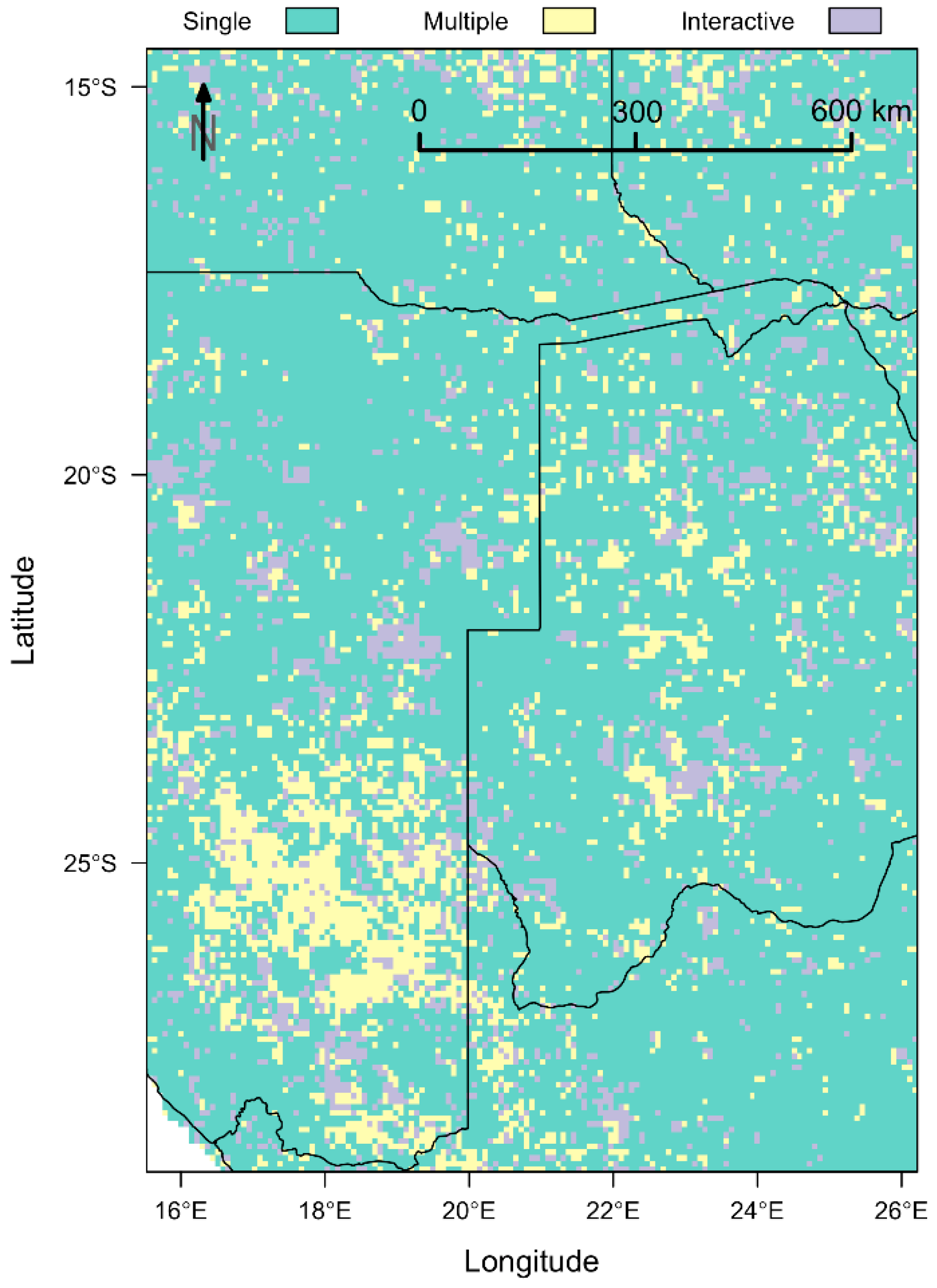
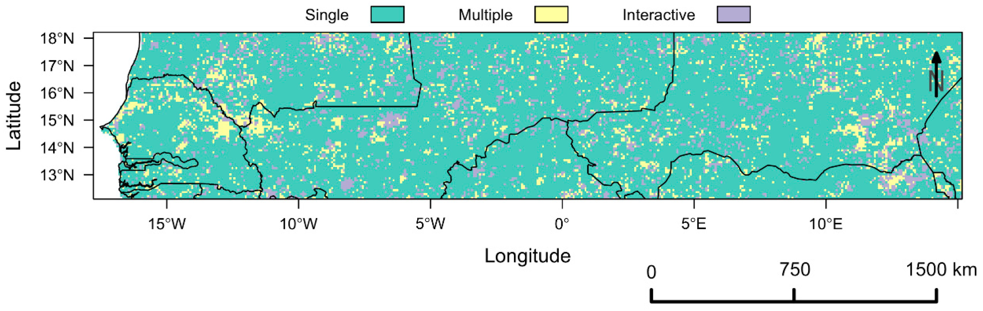
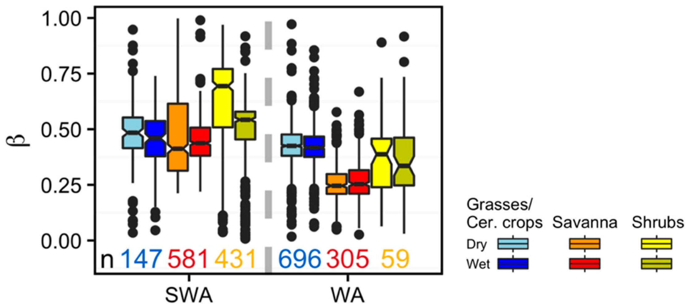
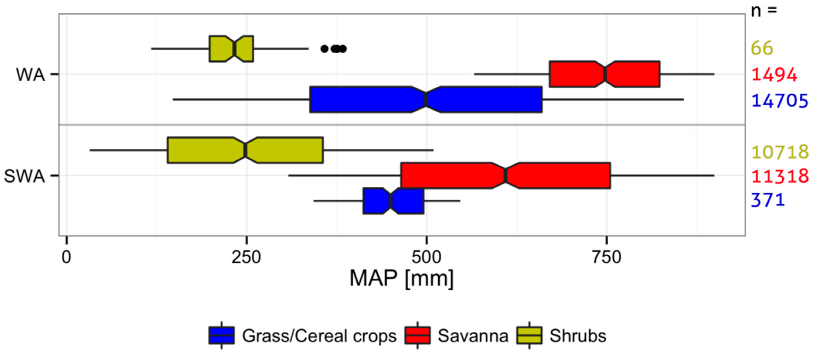
Vegetation Type-Specific Response to Rainfall
4. Discussion
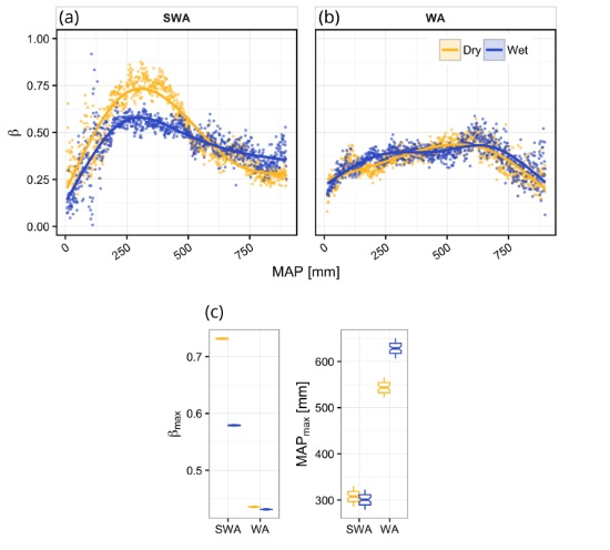
4.1. Vegetation Response to Rainfall Along MAP Gradients
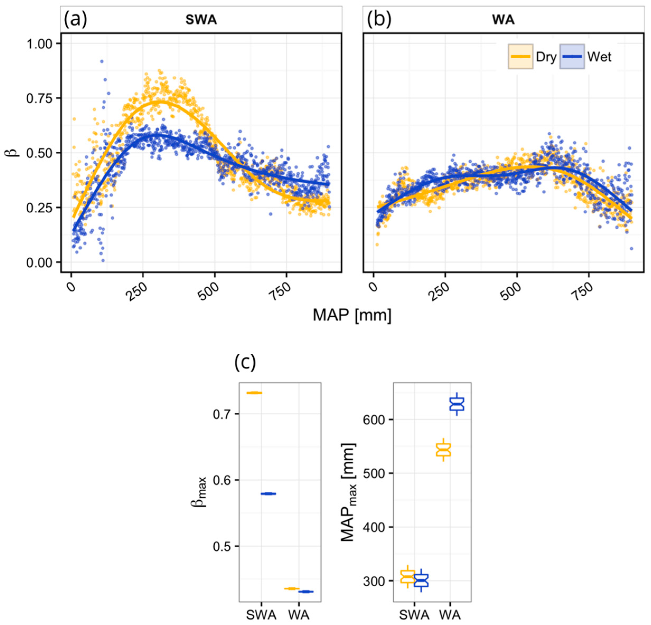
4.2. Dynamics of Peak Vegetation Response to Rainfall
4.3. Vegetation Type-Specific Response to Rainfall
5. Conclusions
Acknowledgments
Author Contributions
Conflicts of Interest
Appendix A
Additional Information on the Study Regions
Appendix B
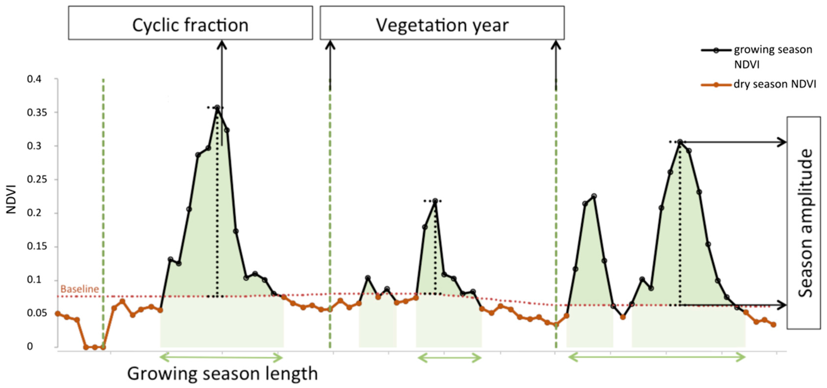
Phenological Parameterization Model
Appendix C
Shifting Linear Regression Model (SLR)

Appendix D
Complementary SLR Analysis

References
- Le Houérou, H.N. Rain use efficiency: A unifying concept in arid-land ecology. J. Arid Environ. 1984, 7, 213–247. [Google Scholar]
- Westoby, M.; Walker, B.; Noy-Meir, I.; Noy-Meir, N. Opportunistic management for rangelands not at equilibrium. J. Range Manag. 1989, 42, 266–274. [Google Scholar] [CrossRef]
- Lauenroth, W.K.; Sala, O.E. Long-term forage production of North American shortgrass steppe. Ecol. Appl. 1992, 2, 397–403. [Google Scholar] [CrossRef] [PubMed]
- Fischer, R.A.; Turner, N.C. Plant productivity in the arid and semiarid zones. Annu. Rev. Plant Physiol. 1978, 29, 277–317. [Google Scholar] [CrossRef]
- Noy-Meir, I. Desert ecosystems: Environments and producers. Annu. Rev. Eclogy Syst. 1973, 4, 25–51. [Google Scholar] [CrossRef]
- Paruelo, J.M.; Lauenroth, W.K.; Burke, I.C.; Sala, O.E. Grassland precipitation-use efficiency varies across a resource gradient. Ecosystems 1999, 2, 64–68. [Google Scholar] [CrossRef]
- McNaughton, S.J.; Oesterheld, M.; Frank, D.A.; Williams, K.J. Ecosystem-level pattern of primary productivity and herbivory in terrestrial habitats. Nature 1989, 341, 142–144. [Google Scholar] [CrossRef] [PubMed]
- Knapp, A.K.; Briggs, J.M.; Collins, S.L.; Archer, S.R.; Bret-Harte, M.S.; Ewers, B.E.; Peters, D.P.; Young, D.R.; Shaver, G.R.; Pendall, E.; et al. Shrub encroachment in North American grasslands: shifts in growth form dominance rapidly alters control of ecosystem carbon inputs. Glob. Chang. Biol. 2008, 14, 615–623. [Google Scholar] [CrossRef]
- Brown, J.H.; Gillooly, J.F.; Allen, A.P.; Savage, V.M.; West, G.B. Toward a metabolic theory of ecology. Ecology 2004, 85, 1771–1789. [Google Scholar] [CrossRef]
- Wang, L.; D’Odorico, P.; Evans, J.P.; Eldridge, D.J.; McCabe, M.F.; Caylor, K.K.; King, E.G. Dryland ecohydrology and climate change: Critical issues and technical advances. Hydrol. Earth Syst. Sci. 2012, 16, 2585–2603. [Google Scholar] [CrossRef] [Green Version]
- Prudhomme, C.; Giuntoli, I.; Robinson, E.L.; Clark, D.B.; Arnell, N.W.; Dankers, R.; Fekete, B.M.; Franssen, W.; Gerten, D.; Gosling, S.N.; et al. Hydrological droughts in the 21st century, hotspots and uncertainties from a global multimodel ensemble experiment. Proc. Natl. Acad. Sci. USA 2014, 111, 3262–3267. [Google Scholar] [CrossRef] [PubMed] [Green Version]
- Weltzin, J.F.; Loik, M.E.; Schwinning, S.; Williams, D.G.; Fay, P.A.; Haddad, B.M.; Harte, J.; Huxman, T.E.; Knapp, A.K.; Lin, G.; et al. Assessing the response of terrestrial ecosystems to potential changes in precipitation. Bioscience 2003, 53, 941–952. [Google Scholar] [CrossRef]
- Jin, Y.; Goulden, M.L. Ecological consequences of variation in precipitation: Separating short-versus long-term effects using satellite data. Glob. Ecol. Biogeogr. 2014, 23, 358–370. [Google Scholar] [CrossRef]
- Verón, S.R.; Oesterheld, M.; Paruelo, J.M. Production as a function of resource availability: Slopes and efficiencies are different. J. Veg. Sci. 2005, 16, 351–354. [Google Scholar] [CrossRef]
- Good, S.P.; Caylor, K.K. Climatological determinants of woody cover in Africa. Proc. Natl. Acad. Sci. USA 2011, 108, 4902–4907. [Google Scholar] [CrossRef] [PubMed]
- Bai, Y.; Wu, J.; Xing, Q.; Pan, Q.; Hunag, J.; Yang, D.; Han, X.; Huang, J. Primary production and rain use efficiency across a precipitation gradient on the mongolia plateau. Ecology 2008, 89, 2140–2153. [Google Scholar] [CrossRef] [PubMed]
- Fensholt, R.; Rasmussen, K. Analysis of trends in the Sahelian “rain-use efficiency” using GIMMS NDVI, RFE and GPCP rainfall data. Remote Sens. Environ. 2011, 115, 438–451. [Google Scholar] [CrossRef]
- Huxman, T.E.; Smith, M.D.; Fay, P.A.; Knapp, A.K.; Shaw, M.R.; Loik, M.E.; Smith, S.D.; Tissue, D.T.; Zak, J.C.; Weltzin, J.F.; et al. Convergence across biomes to a common rain-use efficiency. Nature 2004, 429, 651–654. [Google Scholar] [CrossRef] [PubMed]
- Ponce Campos, G.E.; Moran, M.S.; Huete, A.; Zhang, Y.; Bresloff, C.; Huxman, T.E.; Eamus, D.; Bosch, D.D.; Buda, A.R.; Gunter, S.A.; et al. Ecosystem resilience despite large-scale altered hydroclimatic conditions. Nature 2013, 494, 349–352. [Google Scholar] [CrossRef] [PubMed]
- Verón, S.R.; Paruelo, J.M.; Sala, O.E.; Lauenroth, W.K. Environmental controls of primary production in agricultural systems of the Argentine Pampas. Ecosystems 2002, 5, 625–635. [Google Scholar] [CrossRef]
- Grime, J.P. Plant Strategies, Vegetation Processes and Ecosystem Properties, 2nd ed.; John Wiley & Sons: New York, NY, USA, 2002. [Google Scholar]
- De Wit, C. Transpiration and crop yields. Versl. Van Landbouwkd. Onderz. 1958, 64, 1–88. [Google Scholar]
- Fensholt, R.; Rasmussen, K.; Kaspersen, P.; Huber, S.; Horion, S.; Swinnen, E. Assessing land degradation/recovery in the African Sahel from long-term earth observation based primary productivity and precipitation relationships. Remote Sens. 2013, 5, 664–686. [Google Scholar] [CrossRef] [Green Version]
- Bai, Z.G.; Dent, D.L.; Olsson, L.; Schaepman, M.E. Proxy global assessment of land degradation. Soil Use Manag. 2008, 24, 223–234. [Google Scholar] [CrossRef]
- Prince, S.D.; Brown de Colstoun, E.; Kravitz, L.L. Evidence from rain-use efficiencies does not indicate extensive Sahelian desertification. Glob. Chang. Biol. 1998, 4, 359–374. [Google Scholar] [CrossRef]
- Hsu, J.S.; Powell, J.; Adler, P.B. Sensitivity of mean annual primary production to precipitation. Glob. Chang. Biol. 2012, 18, 2246–2255. [Google Scholar] [CrossRef]
- Camberlin, P.; Martiny, N.; Philippon, N.; Richard, Y. Determinants of the interannual relationships between remote sensed photosynthetic activity and rainfall in tropical Africa. Remote Sens. Environ. 2007, 106, 199–216. [Google Scholar] [CrossRef]
- Hein, L.; De Ridder, N. Desertification in the Sahel: A reinterpretation. Glob. Chang. Biol. 2006, 12, 751–758. [Google Scholar] [CrossRef]
- Chapin, F.S. Effects of plant traits on ecosystem and regional processes: A conceptual framework for predicting the consequences of global change. Ann. Bot. 2003, 91, 455–463. [Google Scholar] [CrossRef] [PubMed]
- Breman, H.; de Wit, C.T. Rangeland productivity and exploitation in the Sahel. Science 1983, 221, 1341–1347. [Google Scholar] [CrossRef] [PubMed]
- Scholes, R.J.; Archer, S.R. Tree-grass interactions in savannas. Annu. Rev. Eclogy Syst. 1997, 28, 517–544. [Google Scholar] [CrossRef]
- Campo-Bescós, M.A.; Muñoz-Carpena, R.; Kaplan, D.A.; Southworth, J.; Zhu, L.; Waylen, P.R. Beyond precipitation: Physiographic gradients dictate the relative importance of environmental drivers on Savanna vegetation. PLoS ONE 2013, 8, 1–14. [Google Scholar]
- Anyamba, A.; Small, J.; Tucker, C.; Pak, E. Thirty-two years of Sahelian zone growing season non-stationary NDVI3g patterns and trends. Remote Sens. 2014, 6, 3101–3122. [Google Scholar] [CrossRef]
- Kaptué, A.T.; Prihodko, L.; Hanan, N.P. On regreening and degradation in Sahelian watersheds. Proc. Natl. Acad. Sci. USA 2015, 112, 12133–12138. [Google Scholar] [CrossRef] [PubMed]
- Holmgren, M.; Hirota, M.; van Nes, E.H.; Scheffer, M. Effects of interannual climate variability on tropical tree cover. Nat. Clim. Chang. 2013, 3, 755–758. [Google Scholar] [CrossRef]
- D’Odorico, P.; Bhattachan, A. Hydrologic variability in dryland regions: Impacts on ecosystem dynamics and food security. Philos. Trans. R. Soc. B Biol. Sci. 2012, 367, 3145–3157. [Google Scholar] [CrossRef] [PubMed]
- Lázaro-Nogal, A.; Matesanz, S.; Godoy, A.; Pérez-Trautman, F.; Gianoli, E.; Valladares, F. Environmental heterogeneity leads to higher plasticity in dry-edge populations of a semiarid Chilean shrub: Insights into climate change responses. J. Ecol. 2015, 103, 338–350. [Google Scholar] [CrossRef]
- Sankaran, M.; Hanan, N.P.; Scholes, R.J.; Ratnam, J.; Augustine, D.J.; Cade, B.S.; Gignoux, J.; Higgins, S.I.; Le Roux, X.; Ludwig, F.; et al. Determinants of woody cover in African savannas. Nature 2005, 438, 846–849. [Google Scholar] [CrossRef] [PubMed]
- Pinzon, J.E.; Tucker, C.J. A non-stationary 1981–2012 AVHRR NDVI3g time series. Remote Sens. 2014, 6, 6929–6960. [Google Scholar] [CrossRef]
- Fensholt, R.; Sandholt, I.; Rasmussen, M.S. Evaluation of MODIS LAI, fAPAR and the relation between fAPAR and NDVI in a semi-arid environment using in situ measurements. Remote Sens. Environ. 2004, 91, 490–507. [Google Scholar] [CrossRef]
- Poulter, B.; Frank, D.; Ciais, P.; Myneni, R.B.; Andela, N.; Bi, J.; Broquet, G.; Canadell, J.G.; Chevallier, F.; Liu, Y.Y.; et al. Contribution of semi-arid ecosystems to interannual variability of the global carbon cycle. Nature 2014, 509, 600–603. [Google Scholar] [CrossRef] [PubMed]
- Brandt, M.; Mbow, C.; Diouf, A.A.; Verger, A.; Samimi, C.; Fensholt, R. Ground and satellite based evidence of the biophysical mechanisms behind the greening Sahel. Glob. Chang. Biol. 2014, 21, 1610–1620. [Google Scholar] [CrossRef] [PubMed]
- Tucker, C.J.; Vanpraet, C.L.; Sharman, M.J.; van Ittersum, G. Satellite remote sensing of total herbaceous biomass production in the Senegalese Sahel: 1980–1984. Remote Sens. Environ. 1985, 17, 233–249. [Google Scholar] [CrossRef]
- Dardel, C.; Kergoat, L.; Hiernaux, P.; Mougin, E.; Grippa, M.; Tucker, C.J. Re-greening Sahel: 30 years of remote sensing data and field observations (Mali, Niger). Remote Sens. Environ. 2014, 140, 350–364. [Google Scholar] [CrossRef]
- Olsen, J.L.; Miehe, S.; Ceccato, P.; Fensholt, R. Does vegetation parameterization from EO NDVI data capture grazing induced variations in species composition and biomass in semi-arid grassland savanna? Biogeosciences 2015, 12, 4407–4419. [Google Scholar] [CrossRef]
- Gangkofner, U.; Brockmann, C.; Brito, J.C.; Campos, J.C.; Wramner, P.; Ratzmann, G.; Fensholt, R.; Günther, K. Vegetation productivity in drylands from Meris fAPAR Time series. In Proceedings of the Sentinel-3 for Science Workshop, Venice, Italy, 2–5 June 2015.
- Novella, N.S.; Thiaw, W.M. African rainfall climatology version 2 for famine early warning systems. J. Appl. Meteorol. Climatol. 2013, 52, 588–606. [Google Scholar] [CrossRef]
- Adler, R.F.; Huffman, G.J.; Chang, A.; Ferraro, R.; Xie, P.; Janowiak, J.; Rudolph, B.; Schneider, U.; Curtis, S.; Bolvin, D.; et al. The version-2 global precipitation climatology project (GPCP) monthly precipitation analysis (1979–Present). J. Hydrometeorol. 2003, 4, 1147–1167. [Google Scholar] [CrossRef]
- Miehe, S.; Kluge, J.; von Wehrden, H.; Retzer, V. Long-term degradation of Sahelian rangeland detected by 27 years of field study in Senegal. J. Appl. Ecol. 2010, 47, 692–700. [Google Scholar] [CrossRef]
- Eamus, D.; Hatton, T.; Cook, P.; Colvin, C. Ecohydrology: Vegetation Function, Water and Resource Management; CSIRO Publishing: Collingwood, Australia, 2006. [Google Scholar]
- De Jong, R.; Schaepman, M.E.; Furrer, R.; de Bruin, S.; Verburg, P.H. Spatial relationship between climatologies and changes in global vegetation activity. Glob. Chang. Biol. 2013, 19, 1953–1964. [Google Scholar] [CrossRef] [PubMed]
- Baldocchi, D.D.; Wilson, K.B. Modeling CO2 and water vapor exchange of a temperate broadleaved forest across hourly to decadal time scales. Ecol. Modell. 2001, 142, 155–184. [Google Scholar] [CrossRef]
- Hastie, T.; Tibshirani, R. Generalized Additive Models: Some applications. J. Am. Stat. Assoc. 1987, 82, 371–386. [Google Scholar] [CrossRef]
- Wood, S.N. Generalized Additive Models, An Introduction with R, 1st ed.; Chapman & Hall/CRC Texts in Statistical Science; CRC Press: Boca Raton, FL, USA, 2006. [Google Scholar]
- R Core Team. R: A Language and Environment for Statistical Computing; R Foundation for Statistical Computing: Vienna, Austria, 2013; Available online: http://www.R-project.org (accessed on 29 August 2014).
- Center for International Earth Science Information Network (CIESIN) Columbia University. Centro Internacional de Agricultura Tropical (CIAT) Gridded Population of the World, Version 3 (GPWv3): Population Density Grid, Future Estimates 2005. Available online: http://dx.doi.org/10.7927/H4ST7MRB (accessed on 2 September 2014).
- Huntley, B.J. Southern African savannas. In Ecology of Tropical Savannas; Huntley, B.J., Walker, B.H., Eds.; Springer: Berlin/Heidelberg, Germany; New York, NY, USA, 1982; pp. 101–119. [Google Scholar]
- Tietjen, B. Same rainfall amount different vegetation—How environmental conditions and their interactions influence savanna dynamics. Ecol. Model. 2016, 326, 13–22. [Google Scholar] [CrossRef]
- Boschetti, M.; Nutini, F.; Brivio, P.A.; Bartholomé, E.; Stroppiana, D.; Hoscilo, A. Identification of environmental anomaly hot spots in West Africa from time series of NDVI and rainfall. ISPRS J. Photogramm. Remote Sens. 2013, 78, 26–40. [Google Scholar] [CrossRef]
- Prince, S.D.; Wessels, K.J.; Tucker, C.J.; Nicholson, S.E. Desertification in the Sahel: A reinterpretation of a reinterpretation. Glob. Chang. Biol. 2007, 13, 1308–1313. [Google Scholar] [CrossRef]
- Le Houérou, H.N. The Grazing Land Ecosystems of the African Sahel, 1st ed.; Springer: Heidelberg, Germany, 1989. [Google Scholar]
- Donohue, R.J.; Roderick, M.L.; McVicar, T.R.; Farquhar, G.D. Impact of CO2 fertilization on maximum foliage cover across the globe’s warm, arid environments. Geophys. Res. Lett. 2013, 40, 3031–3035. [Google Scholar] [CrossRef]
- Huber, S.; Fensholt, R.; Rasmussen, K. Water availability as the driver of vegetation dynamics in the African Sahel from 1982 to 2007. Glob. Planet. Chang. 2011, 76, 186–195. [Google Scholar] [CrossRef]
- Herrmann, S.M.; Anyamba, A.; Tucker, C.J. Recent trends in vegetation dynamics in the African Sahel and their relationship to climate. Glob. Environ. Chang. 2005, 15, 394–404. [Google Scholar] [CrossRef]
- Anyamba, A.; Tucker, C.J. Analysis of Sahelian vegetation dynamics using NOAA-AVHRR NDVI data from 1981–2003. J. Arid Environ. 2005, 63, 596–614. [Google Scholar] [CrossRef]
- Sala, O.E.; Gherardi, L.A.; Reichmann, L.; Jobbágy, E.; Peters, D.; Jobba, E. Legacies of precipitation fluctuations on primary production: Theory and data synthesis. Philos. Trans. R. Soc. Lond. B Biol. Sci. 2012, 367, 3135–3144. [Google Scholar] [CrossRef] [PubMed]
- Thomey, M.L.; Collins, S.L.; Vargas, R.; Johnson, J.E.; Brown, R.F.; Natvig, D.O.; Friggens, M.T. Effect of precipitation variability on net primary production and soil respiration in a Chihuahuan Desert grassland. Glob. Chang. Biol. 2011, 17, 1505–1515. [Google Scholar] [CrossRef]
- Wright, I.J.; Reich, P.B.; Westoby, M. Least-cost input mixtures of water and nitrogen for photosynthesis. Am. Nat. 2003, 161, 98–111. [Google Scholar] [CrossRef] [PubMed]
- Gherardi, L.A.; Sala, O.E. Enhanced precipitation variability decreases grass- and increases shrub-productivity. Proc. Natl. Acad. Sci. USA 2015, 112, 12735–12740. [Google Scholar] [CrossRef] [PubMed]
- Whitford, W.G. Ecology of Desert Ecosystems, 1st ed.; Whitford, W.G., Ed.; Elsevier Science Ltd.: San Diego, CA, USA, 2002. [Google Scholar]
- Ward, D.; Ngairorue, B.T. Are Namibia’s grasslands desertifying? J. Range Manag. 2000, 53, 138–144. [Google Scholar] [CrossRef]
- Lohmann, D.; Tietjen, B.; Blaum, N.; Joubert, D.F.; Jeltsch, F. Shifting thresholds and changing degradation patterns: Climate change effects on the simulated long-term response of a semi-arid savanna to grazing. J. Appl. Ecol. 2012, 49, 814–823. [Google Scholar] [CrossRef]
- Juergens, N.; Oldeland, J.; Hachfeld, B.; Erb, E.; Schultz, C. Ecology and spatial patterns of large-scale vegetation units within the central Namib Desert. J. Arid Environ. 2013, 93, 59–79. [Google Scholar] [CrossRef]
- Verstraete, M.M. Defining desertification: A review. Clim. Chang. 1986, 9, 5–18. [Google Scholar] [CrossRef]
- Nicholson, S.E. The West African Sahel: A review of recent studies on the rainfall regime and its interannual variability. ISRN Meteorol. 2013, 2013, 1–32. [Google Scholar] [CrossRef]
- Dai, A. Drought under global warming: A review. Wiley Interdiscip. Rev. Clim. Chang. 2011, 2, 45–65. [Google Scholar] [CrossRef]
- Hiernaux, P.; Diarra, L.; Trichon, V.; Mougin, E.; Soumaguel, N.; Baup, F. Woody plant population dynamics in response to climate changes from 1984 to 2006 in Sahel (Gourma, Mali). J. Hydrol. 2009, 375, 103–113. [Google Scholar] [CrossRef] [Green Version]
- Scholes, R.J.; Kendall, J.; Justice, C.O. The quantity of biomass burned in southern Africa. J. Geophys. Res. 1996, 101, 23667–23676. [Google Scholar] [CrossRef]
- Biondi, F.; Waikul, K. DENDROCLIM2002: A C++ program for statistical calibration of climate signals in tree-ring chronologies. Comput. Geosci. 2004, 30, 303–311. [Google Scholar] [CrossRef]


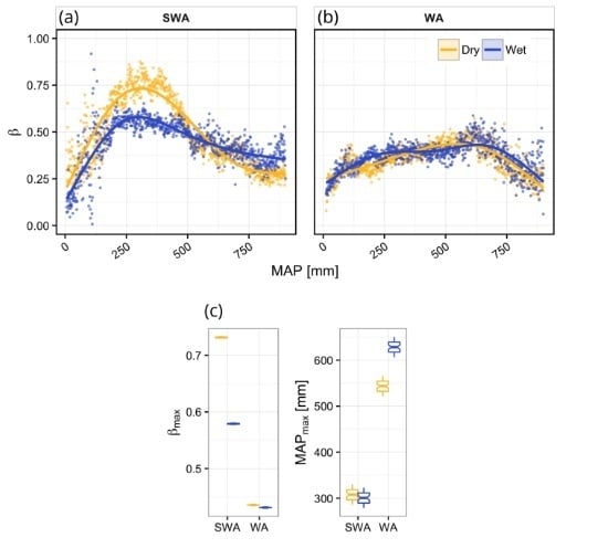
| Region | Clim. | n | p | Edf | R2 | βmax | MAPβ-max |
|---|---|---|---|---|---|---|---|
| SWA | Dry | 893 | <0.001 | 3.98 | 0.84 | 0.73 | 308.0 |
| Wet | 893 | <0.001 | 3.98 | 0.68 | 0.58 | 303.0 | |
| WA | Dry | 888 | <0.001 | 3.91 | 0.67 | 0.44 | 543.5 |
| Wet | 888 | <0.001 | 4.00 | 0.54 | 0.43 | 626.5 |
© 2016 by the authors; licensee MDPI, Basel, Switzerland. This article is an open access article distributed under the terms and conditions of the Creative Commons Attribution (CC-BY) license (http://creativecommons.org/licenses/by/4.0/).
Share and Cite
Ratzmann, G.; Gangkofner, U.; Tietjen, B.; Fensholt, R. Dryland Vegetation Functional Response to Altered Rainfall Amounts and Variability Derived from Satellite Time Series Data. Remote Sens. 2016, 8, 1026. https://doi.org/10.3390/rs8121026
Ratzmann G, Gangkofner U, Tietjen B, Fensholt R. Dryland Vegetation Functional Response to Altered Rainfall Amounts and Variability Derived from Satellite Time Series Data. Remote Sensing. 2016; 8(12):1026. https://doi.org/10.3390/rs8121026
Chicago/Turabian StyleRatzmann, Gregor, Ute Gangkofner, Britta Tietjen, and Rasmus Fensholt. 2016. "Dryland Vegetation Functional Response to Altered Rainfall Amounts and Variability Derived from Satellite Time Series Data" Remote Sensing 8, no. 12: 1026. https://doi.org/10.3390/rs8121026