
Detection of Spatio-Temporal Changes of Norway Spruce Forest Stands in Ore Mountains Using Landsat Time Series and Airborne Hyperspectral Imagery


 ,
,
Abstract
:
1. Introduction
2. Material
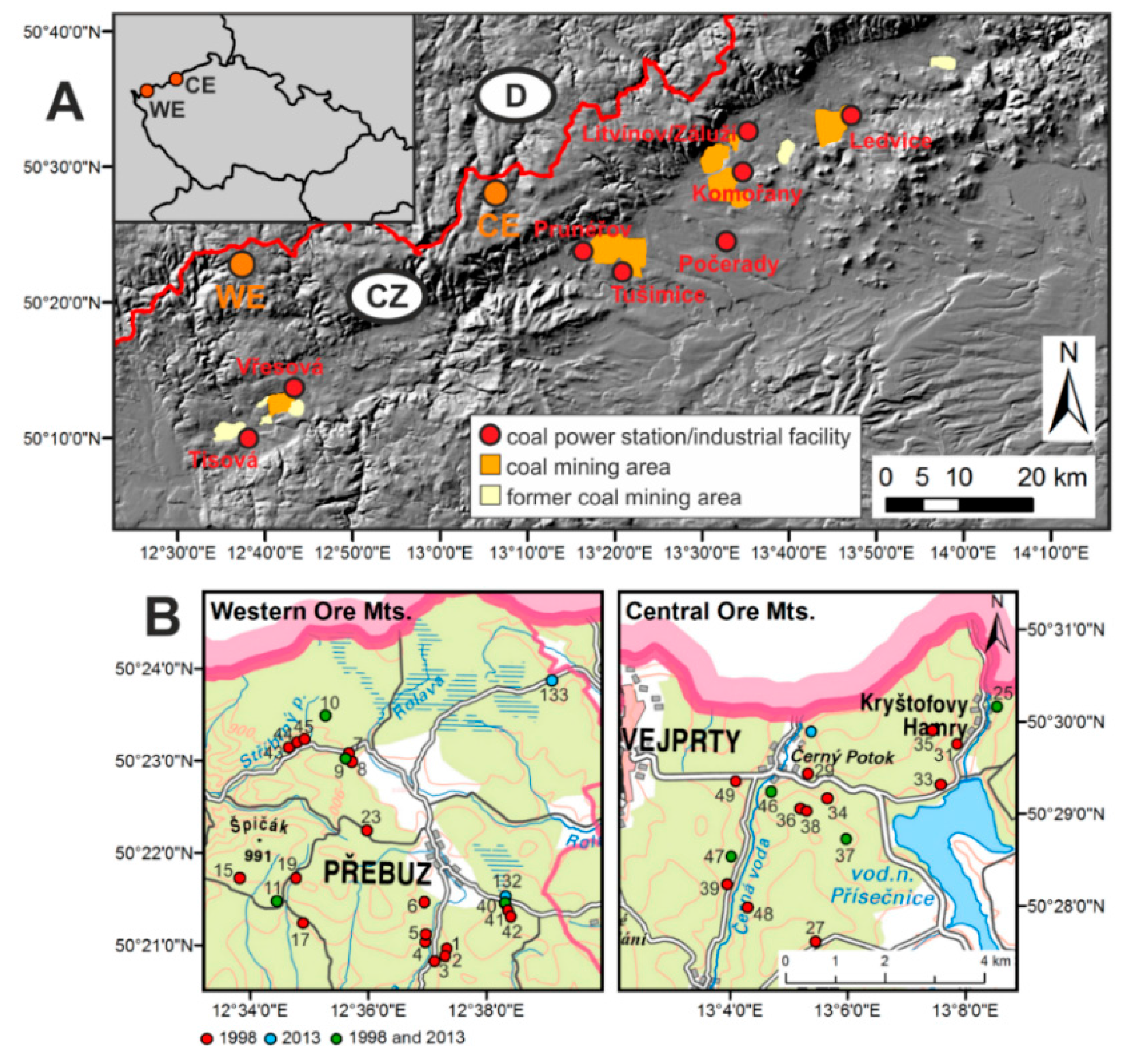
2.1. Study Area

2.2. Landsat Time Series

| 1980s | 1990s | 2000s | 2010s |
|---|---|---|---|
| 13.8.1985 (L5) | 3.3.1990 (L5) | 24.9.2000 (L7) | 30.9.2011 (L7) |
| 31.7.1986 (L5) | 8.8.1992 (L4) | 28.7.2002 (L7) | 15.8.2012 (L7) |
| 14.8.1988 (L5) | 14.7.1994 (L5) | 10.8.2004 (L5) | 2.8.2013 (L7) |
| 7.7.1989 (L5) | 10.8.1998 (L5) | 28.7.2005 (L5) | 6.6.2015 (L8) |
| 13.9.1999 (L7) | 5.9.2006 (L5) | ||
| 24.8.2009 (L5) |
2.3. Airborne Hyperspectral Data
2.4. Field Reference Data
| Damage CLASS | Vitality Status | Canopy Defoliation (%) | |
|---|---|---|---|
| Chlorosis Absent | Chlorosis Present | ||
| DC0 | healthy | 0–10 | no chlorosis |
| DC1 | initial damage | 11–25 | 1–10 |
| DC2 | moderate damage | 26–60 | 11–25 |
| DC3 | heavy damage | 61–80 | 26–60 |
| DC4 | ecosystem collapse | 81–100 | 61–100 |
3. Methods
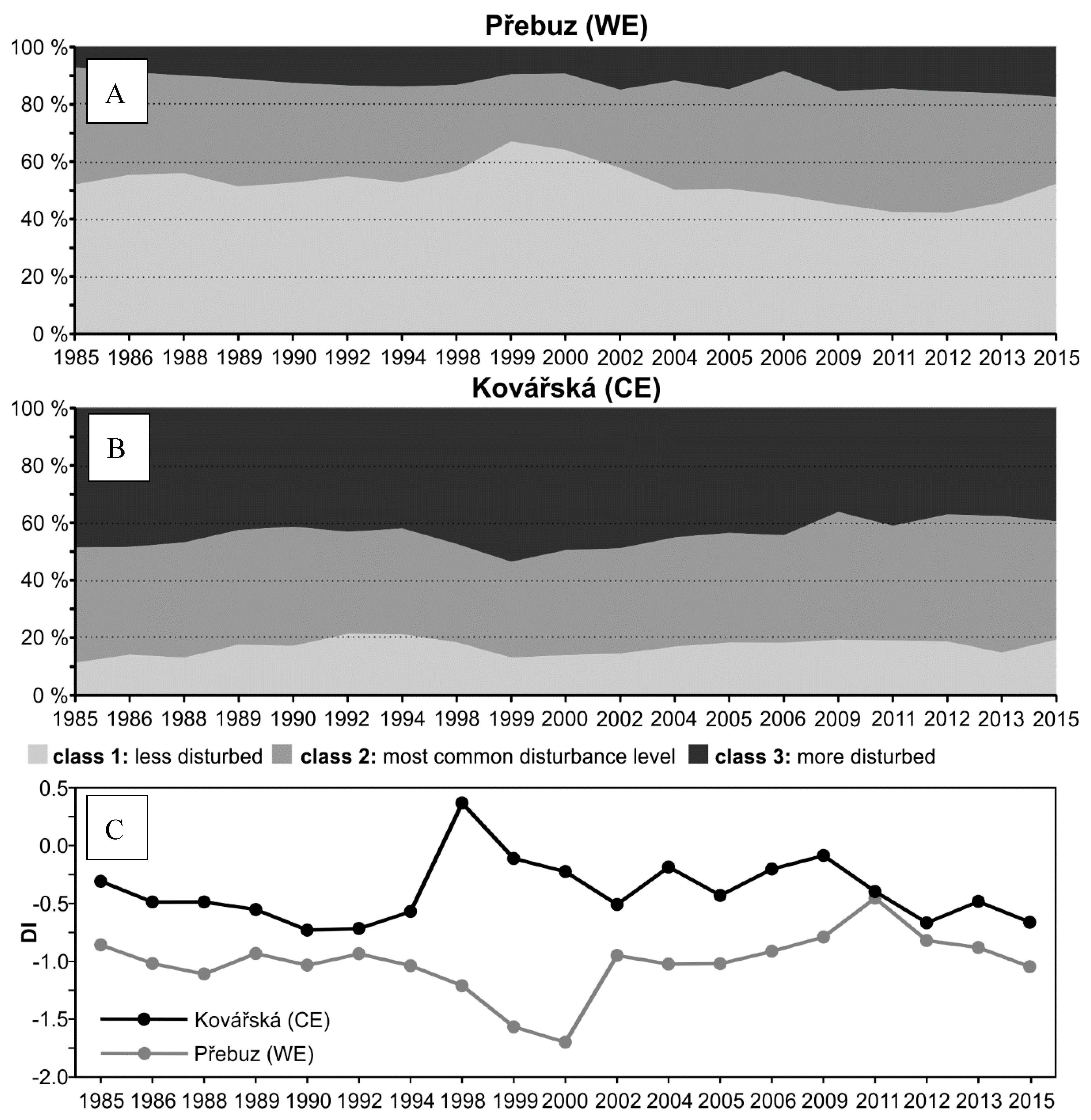
3.1. Landsat Disturbance Index Time Series Analysis
3.2. Vegetation Indices Derived from Hyperspectral Image Data and Stand Separability

| Index | Definition | Reference |
|---|---|---|
| NDVI705 | (R750 − R705)/(R750 + R705) | [46] |
| VOG1 VOG2 | R740/R720 (R734 − R747)/(R715 + R726) | [47] |
| REP | 700 + 40 × ((((R670 + R780)/2) − R700)/(R740 − R700)) | [48] |
| NDVI | (R800 − R670)/(R800 + R670) | [49] |
| RDVI | (R800 − R670)/sqrt(R800 + R670) | [50] |
| MSR | ((R800/R670) − 1)/sqrt((R800/R670) + 1) | [51] |
| MSAVI | 0.5 × (2R800 + 1 − sqrt((2R800 + 1)2 − 8 × (R800 − R670))) | [52] |
| MCARI | ((R700 − R670) − 0.2 × (R700 − R550)) × (R700/R670) | [53] |
| TVI | 0.5 × (120 × (R750 − R550) − 200 × (R670 − R550)) | [54] |
| TCARI | 3 × ((R700 − R670) − 0.2 × (R700 − R550) × (R700/R670)) | [55] |
| OSAVI | ((1 + 0.16)(R800 − R670))/(R800 + R670 + 0.16) | [56] |
| N705 N715 N725 | (R705 − R675)/(R750 − R670) (R715 − R675)/(R750 − R670) (R725 − R675)/(R750 − R670) | [17] |
| D715/D705 D725/D705 | D715/D705 D725/D705 | [17] |
| Rλ stands for reflectance at wavelength λ Dλ stands for 1st derivation of reflectance at wavelength λ | ||
3.3. Detection of Spatio-Temporal Differences
3.4. Statistical Assessment Using Field Reference Data
4. Results
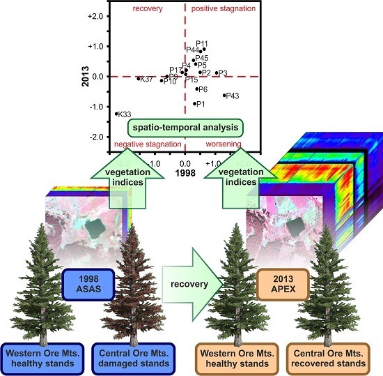
4.1. General Trends of Forest Recovery


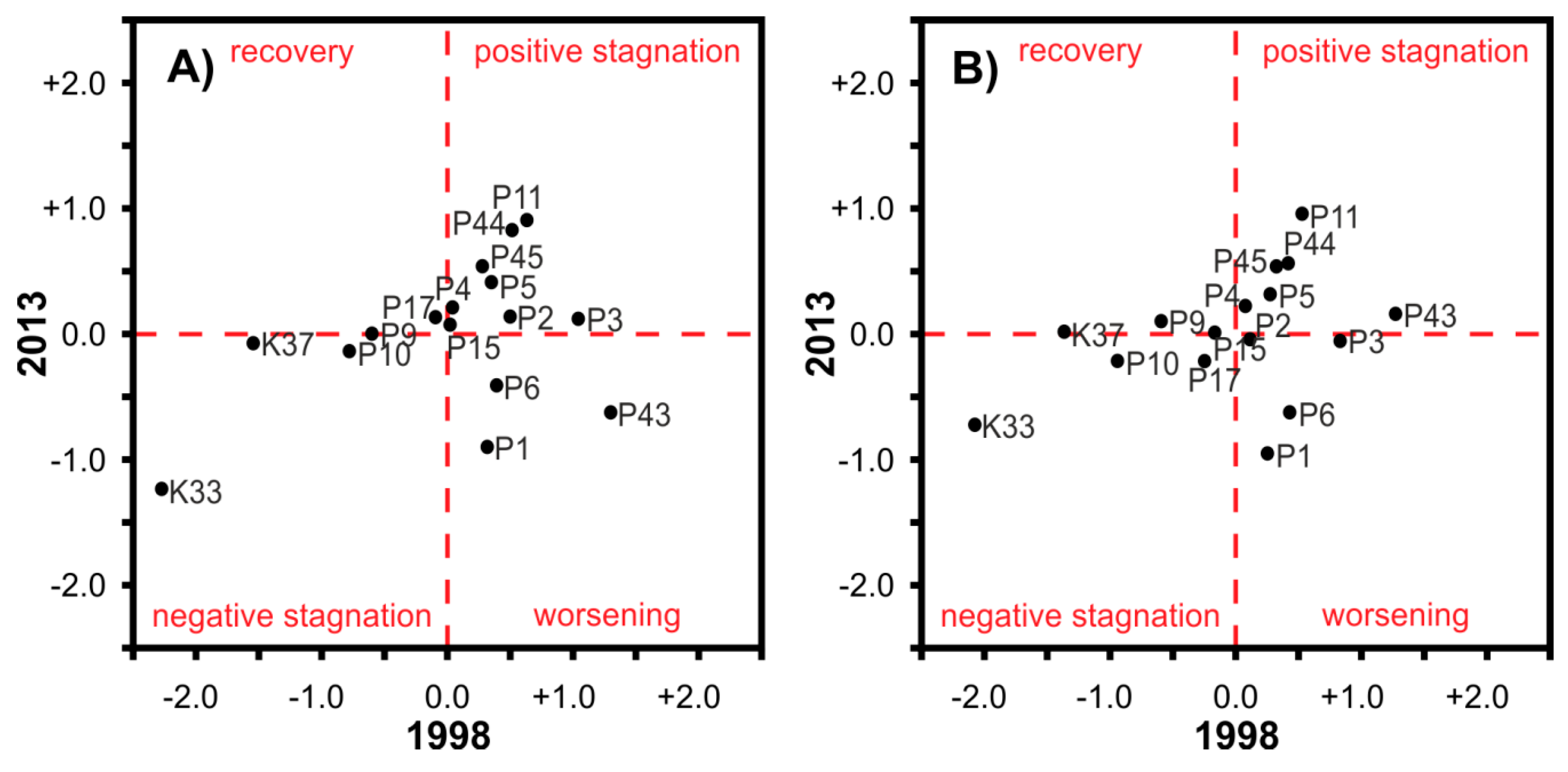
4.2. Assessment of Forest Health Status Change Using ASAS and APEX Datasets

- positive stagnation (+/+): local mean of the normalized VI’ values was positive in both time horizons. The given stand was above the global mean in both years.
- negative stagnation (−/−): local mean of the normalized VI’ values was negative in both years. The stand was below the global mean in both years.
- recovery (−/+): local mean of the normalized VI’ values was negative in 1998, but positive in 2013. The stand was below the global mean in 1998, but above the global mean in 2013.
- worsening (+/−): the given stand was above the global mean in 1998, but below the global mean in 2013.

4.3. Differences in Photosynthetic Pigments Content
| Needle Parameter | 1998 | 2013 | ||
|---|---|---|---|---|
| Western | Central | Western | Central | |
| Chlorophyll a + b (Cab) | 3.61 ± 1.25 a | 3.12 ± 0.68 a | 3.36 ± 0.10 a | 3.66 ± 0.57 a |
| Chlorophyll a/Chlorophyll b (Ca/Cb) | 2.819 ± 0.122 b | 2.902 ± 0.105 a | 2.804 ± 0.144 b | 2.766 ± 0.042 b |
| Total carotenoids/Total chlorophylls (Cx/Cab) | 0.125 ± 0.011 b | 0.136 ± 0.009 a | 0.127 ± 0.008 b | 0.127 ± 0.005 b |
| Relative water content (RWC) | 61.7 ± 5.1 a | 60.0 ± 4.8 ab | 57.4 ± 2.8 b | 58.3 ± 2.7 b |
| Needle Parameter | Effect | ||
|---|---|---|---|
| Year | Site | Year x Site Interaction | |
| Chlorophyll a + b (Cab) | 0.49 n.s. | 0.66 n.s. | 0.05 * |
| Chlorophyll a/Chlorophyll b (Ca/Cb) | <0.01 * | 0.32 n.s. | 0.01 * |
| Total carotenoids/Total chlorophylls (Cx/Cab) | 0.04 * | 0.01 * | <0.01 * |
| Relative water content (RWC) | <0.01 * | 0.61 n.s. | 0.12 n.s. |
5. Discussion
6. Conclusions
Acknowledgments
Author Contributions
Conflicts of Interest
References
- Lambert, N.; Ardo, J.; Rock, B.N. Spectral characterization and regression based classification of forest damage in Norway spruce stands in the Czech Republic using Landsat Thematic Mapper data. Int. J. Remote Sens. 1995, 15, 1261–1287. [Google Scholar] [CrossRef]
- McDonald, A.J.; Gemmel, F.M.; Lewis, P.E. Investigation of the utility of spectral vegetation indices for determining information on coniferous forests. Remote Sens. Environ. 1998, 66, 250–272. [Google Scholar] [CrossRef]
- Asner, G.P. Biophysical and biochemical sources of variability in canopy reflectance. Remote Sens. Environ. 1998, 64, 234–253. [Google Scholar] [CrossRef]
- Pflugmacher, D.; Cohen, W.B.; Kennedy, R.E.; Yang, Z. Using landsat-derived disturbance history and recovery and LiDAR to map forest biomass dynamics. Remote Sens. Environ. 2014, 151, 124–137. [Google Scholar] [CrossRef]
- Muchoney, D.M.; Haack, B.N. Change detection for monitoring forest defoliation. Photogramm. Eng. Remote Sens. 1994, 60, 1243–1251. [Google Scholar]
- Gao, Z.; Gao, W.; Chang, N.B. Integrating temperature vegetation dryness index (TVDI) and regional water stress index (RWSI) for drought assessment with the aid of Landsat TM/ETM plus images. Int. J. Appl. Earth Obs. Geoinform. 2011, 13, 495–503. [Google Scholar] [CrossRef]
- Townsend, P.A.; Eshlemann, K.N.; Welcker, C. Remote estimation of gypsy moth defoliation to assess variations in stream nitrogen concentrations. Ecol. Appl. 2004, 14, 504–516. [Google Scholar] [CrossRef]
- Townsend, P.A.; Singh, A.; Foster, J.R.; Rehberg, N.J.; Kingdon, C.C.; Eshmann, K.N. A general landsat model to predict canopy defoliation on broadleaf deciduous forests. Remote Sens. Environ. 2012, 119, 255–265. [Google Scholar] [CrossRef]
- Kennedy, R.E.; Yang, Z.G.; Cohen, W.B. Detecting trends in forest disturbance and recovery using yearly Landsat time series: 1. LandTrendr−Temporal segmentation algorithms. Remote Sens. Environ. 2010, 114, 2897–2910. [Google Scholar] [CrossRef]
- Main-Knorn, M.; Cohen, W.B.; Kennedy, R.E.; Grodzki, W.; Pflugmacher, D.; Griffiths, P.; Hostert, P. Monitoring coniferous forest biomass change using Landsat trajectory-based approach. Remote Sens. Environ. 2013, 139, 277–290. [Google Scholar] [CrossRef]
- Adams, J.B.; Sabol, D.E.; Kapos, V.; Almeida, R.; Roberts, D.A.; Smith, M.O.; Gillespie, A.R. Classification of multispectral images based on fractions of endmembers—Application to land-cover change in the Brazilian Amazon. Remote Sens. Environ. 1995, 52, 137–154. [Google Scholar] [CrossRef]
- Meddens, A.J.H.; Hicke, J.A.; Vierling, L.A.; Hudak, A.T. Evaluating methods to detect bark beetle-caused tree mortality using single-date and multi-date Landsat imagery. Remote Sens. Environ. 2013, 132, 49–58. [Google Scholar] [CrossRef]
- Schroeder, T.A.; Healey, S.P.; Moisen, G.G.; Frescino, T.S.; Cohen, W.B.; Huang, C.Q.; Kennedy, R.E.; Yang, Z.Q. Improving estimates of forest disturbance by combining observations from Landsat time series with US forest service forest inventory and analysis data. Remote Sens. Environ. 2014, 154, 61–73. [Google Scholar] [CrossRef]
- Cunningham, S.; Rogan, J.; Martin, D.; DeLauer, V.; McCauley, S.; Shatz, A. Mapping land development though periods of economic bubble and bust in Massachusetts using Landsat time series data. GISci. Remote Sens. 2015, 52, 397–415. [Google Scholar] [CrossRef]
- Potapov, P.V.; Turubanova, S.A.; Tyukavina, A.; Krylov, A.M.; McCarty, J.L.; Radeloff, V.C.; Hansen, M.C. Eastern Europe’s forest dynamics from 1985 to 2012 quantified from the full Landsat archive. Remote Sens. Environ. 2015, 159, 28–43. [Google Scholar] [CrossRef]
- Treitz, P.M.; Howarth, P.J. Hyperspectral remote sensing for estimating biophysical parameters of forest ecosystems. Prog. Phys. Geogr. 1999, 23, 359–390. [Google Scholar] [CrossRef]
- Campbell, P.K.E.; Rock, B.N.; Martin, M.E.; Neefus, C.D.; Irons, J.R.; Middleton, E.M.; Albrechtová, J. Detection of initial damage in Norway spruce canopies using hyperspectral airborne data. Int. J. Remote Sens. 2004, 25, 5557–5583. [Google Scholar] [CrossRef]
- Mišurec, J.; Kopačková, V.; Lhotáková, Z.; Hanuš, J.; Weyermann, J.; Entcheva-Campbell, P.; Albrechtova, J. Utilization of hyperspectral image optical indices to assess the Norway spruce forest health status. J. Appl. Remote Sens. 2012, 6. [Google Scholar] [CrossRef]
- Zarco-Tejada, P.J.; Miller, J.R.; Morales, A.; Berjón, A.; Agüera, J. Hyperspectral indices and model simulations for chlorophyll estimation in open-canopy tree crops. Remote Sens. Environ. 2004, 90, 463–476. [Google Scholar] [CrossRef]
- Zhang, Y.; Chen, J.M.; Miller, J.R.; Noland, T.L. Leaf chlorophyll content retrieval from airborne hyperspectral remote sensing imagery. Remote Sens. Environ. 2008, 112, 3234–3247. [Google Scholar] [CrossRef]
- Schlerf, M.; Atzberger, C.; Hill, J.; Buddenbaum, H.; Werner, W.; Schüler, G. Retrieval of chlorophyll and nitrogen content in Norway spruce (Picea abies L. Karst) using imaging spectroscopy. Int. J. Appl. Earth Obs. Geoinform. 2010, 12, 17–26. [Google Scholar] [CrossRef]
- Malenovský, Z.; Homolová, L.; Zurita-Milla, R.; Lukeš, P.; Kaplan, V.; Hanuš, J.; Gastellu-Etchegorry, J.P.; Schaepman, M.E. Retrieval of spruce leaf chlorophyll content from airborne image data using continuum removal and radiative transfer. Remote Sens. Environ. 2013, 131, 85–102. [Google Scholar] [CrossRef]
- Datt, B. Remote sensing of chlorophyll a, chlorophyll b, chlorophyll a + b and total carotenoid content in Eucalyptus leaves. Remote Sens. Environ. 1998, 66, 111–121. [Google Scholar] [CrossRef]
- Gitelson, A.A.; Zur, Y.; Chivkunova, O.B.; Merzlyak, M.N. Assessing carotenoid content in plant leaves with reflectance spectroscopy. Photochem. Photobiol. 2002, 75, 272–281. [Google Scholar] [CrossRef]
- Haboudane, D.; Miller, J.R.; Pattey, E.; Zarco-Tejada, P.J.; Strachan, I.B. Hyperspectral vegetation indices and novel algorithms for predicting green LAI of crop canopies: Modeling and validation in the context of precision agriculture. Remote Sens. Environ. 2004, 90, 337–352. [Google Scholar] [CrossRef]
- Hernandéz-Clemente, R.; Navarro-Cerrillo, R.M.; Zarco-Tejada, P.J. Carotenoid content estimation in a heterogeneous conifer forest using narrow-band indices and PROSPECT+DART simulations. Remote Sens. Environ. 2013, 127, 298–315. [Google Scholar] [CrossRef]
- Govaerts, Y.M.; Verstraete, M.M.; Pinty, B.; Gobron, N. Designing optimal spectral indices: A feasibility and proof of concept study. Int. J. Remote Sens. 1999, 20, 1853–1873. [Google Scholar] [CrossRef]
- Huesca, M.; Merino-de-Miguel, S.; Gonzales-Alonso, F.; Martinez, S.; Cuevas, J.M.; Calle, A. Using AHS hyper-spectral images to study forest vegetation recovery after a fire. Int. J. Remote Sens. 2013, 34, 4025–4048. [Google Scholar] [CrossRef]
- Wu, Y.F.; Hu, X.; Lu, G.H.; Ren, D.C.; Jiang, W.G.; Song, J.Q. Comparison of red edge parameters of winter wheat canopy under late frost stress. Spectrosc. Spectr. Anal. 2014, 34, 2190–2195. [Google Scholar]
- Fassnacht, F.E.; Latifi, H.; Ghosh, A.; Joshi, P.K.; Koch, B. Assessing the potential of hyperspectral imagery to map bark beetle-induced tree mortality. Remote Sens. Environ. 2014. [Google Scholar] [CrossRef]
- Mahlein, A.K.; Rumpf, T.; Welke, P.; Dehne, H.W.; Plumer, L.; Steiner, U.; Oerke, E.C. Development of spectral indices for detecting and identifying plant diseases. Remote Sens. Environ. 2013, 128, 21–30. [Google Scholar] [CrossRef]
- Sanches, I.D.; Souza, C.R.; Kokaly, R.F. Spectroscopic remote sensing of plant stress at leaf and canopy levels using the chlorophyll 680 nm absorption feature with continuum removal. ISPRS J. Photogramm. Remote Sens. 2014, 97, 111–122. [Google Scholar] [CrossRef]
- Behmann, J.; Steinrucken, J.; Plumer, L. Detection of early plant stress responses in hyperspectral images. ISPRS J. Photogramm. Remote Sens. 2014, 93, 98–111. [Google Scholar] [CrossRef]
- Air Pollution and Atmospheric Deposition in Data. Available online: http://portal.chmi.cz/files/portal/docs/uoco/isko/tab_roc/tab_roc_CZ.html (accessed on 4 September 2015).
- Ardo, J.; Lambert, N.; Henzlik, V.; Rock, B.N. Satellite-based estimations of coniferous forest cover changes: Krušné hory, Czech Republic 1972–1989. Ambio 1997, 26, 158–166. [Google Scholar]
- Gege, P.; Fries, J.; Haschberger, P.; Schötz, P.; Schwarzer, H.; Strobl, P.; Suhr, B.; Ulbrich, G.; Vreeling, W.J. Calibration facility for airborne imaging spectrometers. ISPRS J. Photogramm. Remote Sens. 2009, 64, 387–397. [Google Scholar] [CrossRef]
- Schaepman, M.E.; Jehle, M.; Hueni, A.; D’Odorici, P.; Damm, A.; Weyerman, J.; Schneider, F.D.; Laurent, V.; Popp, C.; Seidel, F.C.; et al. Advanced radiometry measurements and earth science applications with the airborne prism experiment (APEX). Remote Sens. Environ. 2015, 158, 207–219. [Google Scholar] [CrossRef]
- Hildebrandt, G.; Gross, C. Remote Sensing Forest Health Status Assessment; European Union, Commision for Agriculture: Walpot, Belgium, 1992. [Google Scholar]
- Porra, R.J.; Thompson, W.A.; Kriedemann, P.E. Determination of accurate extinction coefficients and simultaneous equations for assaying chlorophylls a and b extracted with four different solvents: Verification of the concentration of chlorophyll standards by atomic absorption spectroscopy. Biophys. Biochim. Acta 1989, 975, 384–394. [Google Scholar] [CrossRef]
- Welburn, A.R. The spectral determination of chlorophyll a and b, as well as carotenoids, using various solvents with spectrophotometers of different resolution. J. Plant. Phys. 1994, 144, 307–313. [Google Scholar] [CrossRef]
- Baig, M.H.A.; Zhang, L.; Shuai, T.; Tong, Q. Derivation of tasselled cap transformation based on Landsat 8 at-satellite reflectance. Remote Sens. Lett. 2014, 5, 423–431. [Google Scholar] [CrossRef]
- Liu, Q.S.; Liu, G.H.; Huang, C.; Xie, C.J. Comparison of Tasselled Cap transformations based on the selective bands of Landsat 8 OLI TOA reflectance images. Int. J. Remote Sens. 2015, 36, 417–441. [Google Scholar] [CrossRef]
- Kauth, R.J.; Thomas, G.S. The Tasseled Cap—A graphic description of the spectral—Temporal development of agricultural crops as seen by Landsat. LARS Symp. 1976, 1976, 41–51. [Google Scholar]
- Healey, S.P.; Cohen, W.B.; Yang, Z.; Krankina, O.N. Comparison of Tasseled Cap-based landsat data structure for use in forest disturbance detection. Remote Sens. Environ. 2005, 97, 301–310. [Google Scholar] [CrossRef]
- Tuominen, J.; Lipping, T.; Kuosmanen, V.; Haapanen, R. Remote sensing of forest health. In Remote Sensing of Forest Health, Geoscience and Remote Sensing; Peter Ho, P.-G., Ed.; InTech: Rijeka, Croatia, 2009; pp. 29–52. [Google Scholar]
- Sims, D.A.; Gamon, J.A. Relationships between leaf pigment content and spectral reflectance across a wide range of species, leaf structures and developmental stages. Remote Sens. Environ. 2002, 81, 337–354. [Google Scholar] [CrossRef]
- Vogelmann, J.E.; Rock, B.N.; Moss, D.M. Red edge spectral measurements from Sugar maple leaves. Int. J. Remote Sens. 1993, 14, 1563–1575. [Google Scholar] [CrossRef]
- Curran, P.J.; Windham, W.R.; Gholz, H.L. Exploring the relationship between reflectance red edge and chlorophyll concentration in Slash pine leaves. Tree Phys. 1995, 15, 203–206. [Google Scholar] [CrossRef]
- Rouse, J.W.; Haas, R.H.; Shell, J.A.; Deering, D.W. Monitoring vegetation systems in the Great Plains with ERTS. NASA Spec. Publ. 1974, 351, 309–317. [Google Scholar]
- Roujean, J.L.; Breon, F.M. Estimating PAR absorbed by vegetation from bidirectional reflectance measurements. Remote Sens. Environ. 1995, 51, 375–384. [Google Scholar] [CrossRef]
- Chen, J. Evaluation of vegetation indices and modified simple ratio for boreal applications. Can. J. Remote Sens. 1996, 22, 229–242. [Google Scholar] [CrossRef]
- Qi, J.; Chehbouni, A.; Huete, A.R.; Keer, Y.H.; Sorooshian, S.A. A modified soil vegetation adjusted index. Remote Sens. Environ. 1994, 48, 119–126. [Google Scholar] [CrossRef]
- Daughtry, C.S.T.; Walthall, C.L.; Kim, M.S.; Brown de Colstoun, E.; McMuetrey, J.E., III. Estimating corn leaf chlorophyll concentration from leaf and canopy reflectance. Remote Sens. Environ. 2000, 74, 229–239. [Google Scholar] [CrossRef]
- Broge, N.H.; Leblanc, E. Comparing prediction power and stability of broadband and hyperspectral vegetation indices for estimating of green leaf area index and canopy chlorophyll density. Remote Sens. Environ. 2000, 76, 156–172. [Google Scholar] [CrossRef]
- Haboudane, D.; Miller, J.R.; Tremblay, N.; Zarco-Tejada, P.J.; Dextraze, L. Integrated narrow-band vegetation indices for prediction of crop chlorophyll content for application to precision agriculture. Remote Sens. Environ. 2002, 81, 416–426. [Google Scholar] [CrossRef]
- Rondeaux, G.; Steven, M.; Baret, F. Optimization of soil-adjusted vegetation indices. Remote Sens. Environ. 1996, 55, 95–107. [Google Scholar] [CrossRef]
- Konečná, B.; Frič, F.; Masarovičová, E. Ribulose-1,5-bisphosphate carboxylase activity and protein content in pollution damaged leaves of three oak species. Photosynthetica 1989, 23, 566–574. [Google Scholar]
- Siefermann-Harms, D. Light and temperature control of season-dependent changes in the α- and β-carotene content of spruce needles. J. Plant. Phys. 1994, 143, 488–494. [Google Scholar] [CrossRef]
- Kopačková, V.; Mišurec, J.; Lhotáková, Z.; Oulehle, F.; Albrechtová, J. Using multi-date high spectral resolution data to assess physiological status of macroscopically undamaged foliage on a regional scale. Int. J. Appl. Earth Obs. Geoinform. 2014, 27, 169–186. [Google Scholar] [CrossRef]
- Kopačková, V.; Lhotáková, Z.; Oulehle, F.; Albrechtová, J. Assessing forest health via linking the geochemical properties of soil profile with the biochemical parameters of vegetation. Int. J. Environ. Sci. Technol. 2015, 12, 1987–2002. [Google Scholar] [CrossRef]
- Soukupová, J.; Cvikrová, M.; Albrechtová, J.; Rock, B.N.; Eder, J. Histochemical and biochemical approaches to the study of phenolic compounds and peroxidases in needles of Norway spruce (Picea Abies). New Phytol. 2000, 146, 403–414. [Google Scholar] [CrossRef]
- Cudlín, P.; Novotný, R.; Moravec, I.; Chmelíková, E. Retrospective evaluation of the response of montane forest ecosystems to multiple stress. Ekológia 2001, 20, 108–124. [Google Scholar]
- Polák, T.; Cudlín, P.; Moravec, I.; Albrechtová, J. Macroscopic indicators for the retrospective assessment of Norway spruce crown response to stress in the Krkonoše Mountains. Trees 2007, 21, 23–35. [Google Scholar] [CrossRef]
- Program Ekologizace. Available online: http://www.cez.cz/cs/odpovedna-firma/zivotni-prostredi/programy-snizovani-zateze-zp/snizovani-znecisteni-ovzdusi/program-ekologizace.html (accessed on 23 November 2015).
- Mylona, S. Sulphur dioxide emissions in Europe 1880–1991 and their effect on sulphur concentrations and depositions. Tellus. Ser. B-Chem. Phys. Meteorol. 1996, 48, 662–689. [Google Scholar] [CrossRef]
- Kubíková, J. Forest dieback in Czechoslovakia. Vegetation 1991, 93, 101–108. [Google Scholar] [CrossRef]
- Šrámek, V.; Slodičák, M.; Lomský, B.; Balcar, V.; Kulhavý, J.; Hadaš, P.; Pulkráb, K.; Šišák, L.; Pěnička, L.; Sloup, M. The Ore Mountains: Will successive recovery from lethal disease be successful? Mt. Res. Dev. 2008, 28, 216–221. [Google Scholar]
- Bytnerowicz, A.; Omasa, K.; Paoletti, E. Integrated effects of air pollution and climate on forests: A northern hemisphere perspective. Environ. Pollut. 2007, 147, 438–445. [Google Scholar] [CrossRef] [PubMed]
- Paoletti, E.; Schaub, M.; Matyssek, R.; Wieser, G.; Augustaitis, A.; Bastrup-Birk, A.M.; Bytnerowicz, A.; Günthardt-Georg, M.S.; Müller-Starck, G.; Serengil, Y. Advances of air pollution sciences: From forest decline to multiple stress effects on forest ecosystem services. Environ. Pollut. 2010, 158, 1986–1989. [Google Scholar] [CrossRef] [PubMed]
© 2016 by the authors; licensee MDPI, Basel, Switzerland. This article is an open access article distributed under the terms and conditions of the Creative Commons by Attribution (CC-BY) license (http://creativecommons.org/licenses/by/4.0/).
Share and Cite
Mišurec, J.; Kopačková, V.; Lhotáková, Z.; Campbell, P.; Albrechtová, J. Detection of Spatio-Temporal Changes of Norway Spruce Forest Stands in Ore Mountains Using Landsat Time Series and Airborne Hyperspectral Imagery. Remote Sens. 2016, 8, 92. https://doi.org/10.3390/rs8020092
Mišurec J, Kopačková V, Lhotáková Z, Campbell P, Albrechtová J. Detection of Spatio-Temporal Changes of Norway Spruce Forest Stands in Ore Mountains Using Landsat Time Series and Airborne Hyperspectral Imagery. Remote Sensing. 2016; 8(2):92. https://doi.org/10.3390/rs8020092
Chicago/Turabian StyleMišurec, Jan, Veronika Kopačková, Zuzana Lhotáková, Petya Campbell, and Jana Albrechtová. 2016. "Detection of Spatio-Temporal Changes of Norway Spruce Forest Stands in Ore Mountains Using Landsat Time Series and Airborne Hyperspectral Imagery" Remote Sensing 8, no. 2: 92. https://doi.org/10.3390/rs8020092
APA StyleMišurec, J., Kopačková, V., Lhotáková, Z., Campbell, P., & Albrechtová, J. (2016). Detection of Spatio-Temporal Changes of Norway Spruce Forest Stands in Ore Mountains Using Landsat Time Series and Airborne Hyperspectral Imagery. Remote Sensing, 8(2), 92. https://doi.org/10.3390/rs8020092