Article

Evaluating the Effectiveness of Conservation on Mangroves: A Remote Sensing-Based Comparison for Two Adjacent Protected Areas in Shenzhen and Hong Kong, China

1
Key Laboratory of Wetland Ecology and Environment, Northeast Institute of Geography and Agroecology, Chinese Academy of Sciences, Changchun 130102, China
2
University of Chinese Academy of Sciences, No. 19, Yuquan Road, Beijing 100049, China
3
School of Geographical Sciences, Guangzhou University, Guangzhou 510006, China
*
Authors to whom correspondence should be addressed.
These authors contributed equally to this work.
Remote Sens. 2016, 8(8), 627; https://doi.org/10.3390/rs8080627
Submission received: 29 February 2016 / Revised: 27 June 2016 / Accepted: 22 July 2016 / Published: 29 July 2016
(This article belongs to the Special Issue What can Remote Sensing Do for the Conservation of Wetlands?)

Abstract

:
Mangroves are ecologically important ecosystems and globally protected. The purpose of this study was to evaluate the effectiveness of mangrove conservation efforts in two adjacent protected areas in China that were under the management policies of the Ramsar Convention (Mai Po Marshes Nature Reserve (MPMNR), Hong Kong) and China’s National Nature Reserve System (Futian Mangrove National Nature Reserve (FMNNR), Shenzhen). To achieve this goal, eleven Landsat images were chosen and classified, areal extent and landscape metrics were then calculated. The results showed that: from 1973–2015, the areal extent of mangroves in both reserves increased, but the net change for the MPMNR (281.43 hm2) was much higher than those of the FMNNR (101.97 hm2). In general, the area-weighted centroid of the mangroves in FMNNR moved seaward by approximately 120 m, whereas in the MPMNR, the centroid moved seaward even farther (410 m). Although both reserves saw increased integrality and connectivity of the mangrove patches, the patches in the MPMNR always had higher integrality than those in the FMNNR. We concluded that the mangroves in the MPMNR were more effectively protected than those in the FMNNR. This study may provide assistance to the formulation of generally accepted criteria for remote sensing-based evaluation of conservation effectiveness, and may facilitate the development of appropriate mangrove forest conservation and management strategies in other counties.

Graphical Abstract

1. Introduction

Mangroves are tropical trees and shrubs that grow in sheltered coastlines, mudflats, and river banks in many parts of the world [1]. These forests play an important role in stabilizing shorelines and help reduce the devastating impacts of natural disasters such as tsunamis, and hurricanes [2]. They also provide important ecological and societal goods and services, including breeding and nursing grounds for marine and pelagic species, food, medicine, fuel, and building materials for local communities. Despite the wide range of ecological and socio-economic benefits, mangroves have become a plant in peril [3,4]. Over the last two decades of the 20th century, the area of the world’s mangrove forests has decreased by 35% [5]. Vast areas of mangrove forests have been cleared for urban development, industrialization, agricultural land reclamation, timber and charcoal production, and shrimp farming [6]. The remaining mangrove forests are also under pressure from clear cutting, encroachment, hydrological alterations, chemical spills, and climate change [7]. It was not until the 1980s that significant efforts were taken to protect and manage this unique and valuable ecosystem. However, there were few studies focused on conditions of mangrove wetlands conservation. Updated information concerning the extent and condition of mangrove forests under protection should be retrieved to aid in forest management and in policy- and decision-making processes [8].
Remote sensing provides many advantages over field surveys in monitoring inaccessible coastal ecosystems and, in addition, the method is accurate, rapid, and cost effective [9]. Numerous studies on remote sensing-based mapping of mangroves have been published over the last two decades [10]. According to the literature, various remote sensing data have been applied in mapping and understanding changes in the areal extent and spatial pattern of mangrove forests, categorized by sensor types: airborne photograph [11], optical medium-resolution [12], optical high-resolution [13], hyperspectral [14], and radar data [15]. Although aerial photography, high-resolution satellite imagery, hyperspectral, and radar data partially provide information with details, some national agencies are more interested in updated overview information on a regional or even a country-wide scale [16] because reports of status and trends in a long term could support their spatial planning and conservation-planning tasks. Medium-resolution imagery, which delivers appropriate coverage and information, has advantages in achieving national agencies’ objectives.
Among various medium-resolution satellite data, Landsat series images have been most widely used to detect mangrove forest changes in many regions, including the Sundarbans of Bangladesh and India [2], the Brazilian Amazon [17], Vietnam [18], Philippines [19], and even the entire world [20]. Although the coarse spatial resolution of the Landsat data is actually not well suited for species-level mapping, these data were adaptive for applying dynamics studies [21]. Jia and colleagues estimated mangrove forests loss and restoration due to natural and anthropogenic factors in Guangxi, China, using Landsat data acquired in 1973, 1981, 1990, 2000, and 2010, and provided valuable information for understanding factors causing mangrove forest dynamics [22]. Wang et al. used Landsat TM (1990) and ETM+ (2000) images to identify changes in distribution and total area occupied by mangroves along the Tanzanian coast, and demonstrated that remote sensing and GIS can offer important data and tools in the advancement of coastal resource management and ecosystem monitoring [23]. The most advantage of Landsat data is that they are freely and continuously available for a long time span (the last four decades) in contrast to the cost-intensive and short time span of other remote sensing data [24].
For more than two decades, various remote sensing-based methodologies have been used to obtain the condition and extent of mangrove ecosystems. The methods were applied exclusively or in combination [10]. Traditional mapping methods consisting of visual-interpretation analyses and on-screen digitizing were used extensively to map mangrove forests. Additionally, visual-interpretation has been used as an auxiliary method in modifying classification results generated by unsupervised or supervised classification methodologies. For example, Jia et al. applied visual-interpretation after China’s mangroves were extracted by nearest neighbor classifiers (a supervised classification method) and finally obtained an overall accuracy of 93% [24]. Various classification algorithms have been investigated or compared for the suitability of spectral separation of the mangrove forests, such as the supervised Maximum Likelihood Classifier [25], Principal Component Analysis [26], Neural Networks [27], Spectral Angle Mapping [28], and Band Combination Methods [29]. Using these techniques, most studies reported classification accuracies of 75%–90% for producers and users [30].
However, in recent years, an increasing dissatisfaction with pixel-based image analysis has been identified [31], among which the most questioned disadvantage is that the pixel-based approach causes a salt-and-pepper effect, leading to the erroneous classification of pixels [32,33]. Object-based classification is a technique that uses objects, rather than only individual pixels for image analysis. Thus, objects have additional spectral information compared to single pixels (e.g., mean values per band, as well as median values, minimum and maximum values, mean ratios, and variance), but of even greater advantage than the diversification of spectral value descriptions of objects is the additional spatial information for such objects as distances, neighborhoods, and topologies [34]. Once the objects have been obtained, they will be classified based on spectral, spatial, textural, relational, and contextual features. The object-based classification method was primarily used in interpreting high resolution images, but according to recent literature, this method was also used for medium-resolution images classification. For example, Berlanga-Robles and Ruiz-Luna [35] performed a multi-temporal landscape change detection on the Mexican Pacific coast with Landsat MSS and TM data from 1973–1997. Conchedda et al. [36] mapped land cover in Low Casamance, Senegal using SPOT XS data and object-based classification methods. Additionally, Jia et al. applied an object-based method and Landsat images to map mangrove forests and other coastal land covers in China [22,24]. The benefits resulting from object-based classification of remotely-sensed images are widely demonstrated, such as overcoming salt-and-pepper effects [37], and providing geo-information that can be immediately stored into Geographical Information System (GIS) databases [38]. Furthermore, this process is usually fast and of high classification accuracy because image objects, rather than individual pixels are assigned to specific classes [39].
The geographic proximity of Futian and Mai Po make them ideal test sites for evaluating and comparing the efficacies of the various protection policies. The primary aim of our study is to compare the protection effectiveness of two protected areas under different conservation policies (see Section 2) using a remote sensing-based methodology.

2. Background: Mangrove Conservation Projects

The Ramsar Convention on Wetlands is the most famous and widely adopted wetlands protection project. Established in response to the large-scale and widespread destruction of marshes and wetlands throughout Europe, the Convention on Wetlands of International Importance, especially as Waterfowl Habitat was signed in 1971 in Ramsar, Iran [8]. Currently, 169 countries have signed the convention, which lists 2241 designated sites with a total surface area of 215,247,631 hm2 [40]. China is the first developing country to declare the adoption of a sustainable development strategy [41]. To protect its environment, China has established over 2000 national and local nature reserves, mostly within the last 20 years [42,43]. Among those reserves, China’s National Nature Reserves (CNNR), which are on the list of priority financial and political projects, were established on the approval of the State Council. As of early 2015, there were 428 CNNRs that covered approximately 100 million hectares, which is approximately 10% of the country’s land surface [44].
As a unique wetland ecosystem, mangroves have been the priority for protection by the Ramsar Convention and CNNRs. This study chose the Futian Mangrove National Nature Reserve (FMNNR) and Mai Po Marshes Nature Reserve (MPMNR) to evaluate and compare conservation efficacies of the Ramsar Convention and CNNRS. The MPMNR has been managed by the World Wide Fund for Nature Hong Kong (WWFHK) since 1983 and was added as a Wetland of International Importance under the Ramsar Convention in September 1995 [45,46]. To protect birds and vegetation better in Mai Po, the whole MPMNR was closed to the public. Figure 1 shows photos of Mai Po mangroves and Futian Mangroves. In 1984, the FMNNR was established in Shenzhen, Guangdong province, China, and, in 1988 it was approved as a mangrove CNNR. Large parts of the FMNNR have been opened to the public as a wetland park. Vegetation includes mangroves, semi-mangrove and seashore plants, with Aegiceras corniculatum, Kandelia candel and Avicennia marina being the dominant native mangrove species, and Sonneratia caseolaris and Sonneratia apetala being exotic mangrove species [47]. Futian mangroves were seriously threatened by a population explosion. In 1980, there were only 30,000 residents, but by 2008, the city had 12 million inhabitants.

3. Materials and Methods
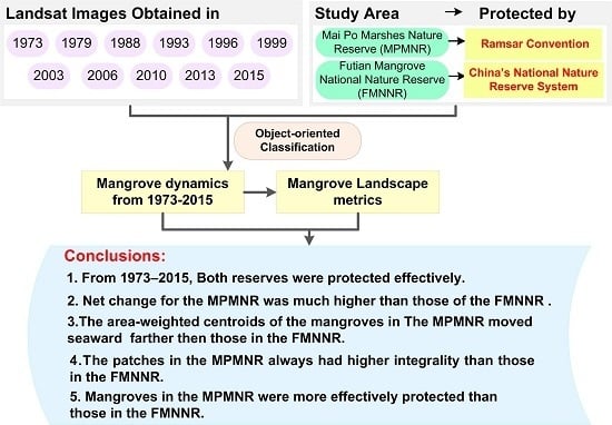
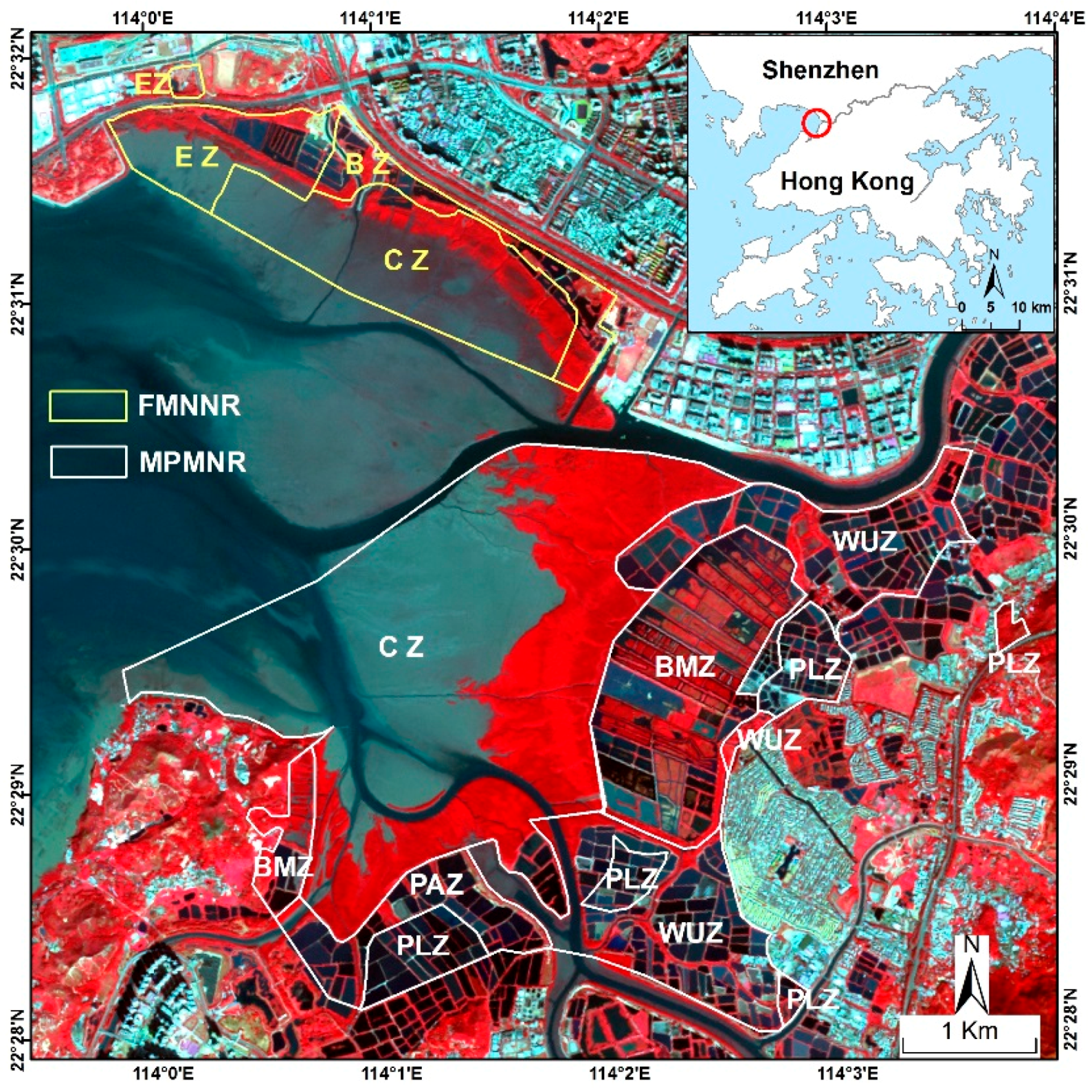
3.1. Study Area

The MPMNR and FMNNR are situated in the northwestern part of the New Territories of Hong Kong and in Southern Shenzhen, respectively, and they are separated by the Shenzhen River (Figure 2). Both are located in the Pearl River Delta, bordering the mudflats and mangrove forests of the Inner Deep Bay and are generally influenced by the Pearl River. The climate is largely governed by mainland China and the South China Sea. Summers are hot and humid with winds from the south and southeast, and winters are mild and relatively dry. The MPMNR and FMNNR are well known for their importance as a wintering ground and stop-over point for migrating birds on the East Asian–Australasian Flyway. Each year, more than 55,000 migrating birds, including over ten globally-threatened species, pass through these mangroves [48]. Due to the ecological importance of these nature reserves, their environmental quality has been of concern to local governments, the media, and environmental activists [49].
As managed under the Ramsar treaties, the MPMNR was divided into five different management zones by the Agriculture, Fisheries, and Conservation Department (AFCD) of Hong Kong based on the habitat types, ecological values and existing land uses: the Core Zone (CZ), Biodiversity Management Zone (BMZ), Wise Use Zone (WUZ), Public Access Zone (PAZ), and Private Land Zone (PLA, Figure 2). This study only focused on the CZ, which is mainly dominated by the large number of mangrove forests that border the sea.
As a CNNR, the FMNNR was divided into three zones: Core zone (CZ), Buffer zone (BZ) and Experimental zone (EZ, Figure 2). In principle, human activities are limited in the EZs and BZ, and no human activity is allowed in the CZ. Due to the small area of FMNNR, this study focused on all of the mangrove forests along the beach of the FMNNR.

3.2. Data Preparation

In this study, multispectral Landsat images with a moderate resolution of 30 m/60 m were chosen to monitor long-term changes in the MPMNR and FMNNR mangrove forests. Cloud-free Landsat images obtained between 1973 and 2015 were downloaded from the USGS Center for Earth Resources Observation and Science [50]. All Landsat data are nominally processed as Level 1 terrain-corrected (L1T) data, which provides systematic radiometric and geometric accuracy by incorporating ground control points, while also employing a digital elevation model (DEM) for topographic accuracy [50]. A complete list of the Landsat Multi-spectral Scanner (MSS), Thematic Mapper (TM), and Enhanced Thematic Mapper Plus (ETM+) data used in this study is shown in Table 1. For each year, the entire area of the study area was covered using one Landsat scene. Moreover, most of the images were acquired with instantaneous tidal heights of less than 0.5 m, which indicates that nearly all of the mangrove canopies were exposed above the sea surface.
Although the Landsat images were already geo-referenced, the images could not be directly compared because the resolutions and coordinate reference systems used in the images were inconsistent. In order to standardize the dataset, and keep spatial details, MSS images were resampled to a pixel size of 30 m × 30 m. Although the spatial information cannot be truly downscaled, pixel size of these MSS images is consistent with other Landsat images. Next all images were projected to the Universal Transverse Mercator (UTM) coordinate system. To reduce potential position errors between the images, we initially geo-rectified the Landsat images obtained in 2010 using a 1:50,000 topographic map. Using the geo-rectified images as a master dataset, we resampled and rectified the Landsat images obtained in 1973, 1979, 1988, 1993, 1996, 1999, 2003, 2006, 2010, 2013, and 2015. An average root mean square error (RMSE) of less than 0.5 pixels was obtained for the co-registered images. The FLAASH module (a module in ENVI software [51]) was used for atmospheric corrections of Landsat images [52]. Input into the FLAASH module includes the average elevation of the study area, scene center coordinates, sensor type, flight date and time, atmospheric model, and information about aerosol distribution, visibility, and water vapor conditions. In this study, scene center coordinates, sensor type, flight date and time were set according to the metafile of images. For all images, the average elevation of the study area was set to 0, and atmospheric model was set to Tropical. When selecting an aerosol model, images in 1973, 1979, and 1988 were set to the rural model, and other images were set to the urban model. The visibility and water vapor conditions were set as default values. In this study, ENVI software [51] was used to perform the geo-rectification and atmospheric corrections on the Landsat images.
Ground surveys were conducted in Shenzhen and Hong Kong during October and November 2013. We also collected ground truth points from high-resolution images available on Google Earth. The samples contained 110 points of mangroves and 255 points of other land cover types. Among these pointes, 22 and 80 mangrove and non-mangrove points, respectively (with a minimum of 10 points per land cover type), were collected as training samples during the classification. The remaining 88 mangrove points and 175 non-mangrove points were used to validate the accuracy of the classification results in 2013. Field data, photos, interviews with local experts and residents, and e-mails from local experts, as well as various historic maps were used as reference data in the assessment of the classification results in other years. The historic maps were firstly digitized by ArcGIS software [53], and ground truth points were subsequently from the digital maps. These ground truth points contained spatial location and land cover types. The ground truth points are shown in Table 2.

3.3. Methodology

An image-analysis program (eCognition Developer [54]) was used to perform the object-oriented classification. The first step of the object-oriented method is segmentation, which is the process of segmenting an image into groups of homogeneous pixels such that the variability within the object is minimized [55]. In this study a multi-resolution segmentation method was used. Image segmentation parameters include scale, shape, and compactness. The scale determines the maximum size of the created object, the shape factor balances spectral homogeneity vs. the shape of the objects, and the compactness factor balances the compactness and smoothness [56]. Users can apply weights from 0 to 1 to the shape and compactness factors to determine objects at a certain level of scale. Mangrove objects are irregularly shaped, and less weight was therefore assigned to the shape than to the spectral homogeneity (the shape factor was set to 0.1). The compactness parameter was set at 0.6 to give a little more weight to compactness than smoothness. Since the scale parameter is an important variable for defining the break off value for spectral homogeneity, it has to be determined before segmentation. From our previous experiments, after a series of tests, a satisfactory match between image objects and landscape features was achieved when the scale parameter was determined to be 8.
After the objects in the images were segmented, the image objects were classified into mangrove and other land cover types using nearest neighbor (NN) classifiers and visual interpretation [57]. In NN classifier processing, training samples were selected in the same scene and were subjected to classification to avoid spectral differences caused by various sensors. General shapes of the spectral curves of mangroves and other vegetation are similar, with considerable overlap in bands 1–3 (450 nm–690 nm). In the spectral range of band 4 (760 nm–900 nm), the reflectance of coastal farmland was higher than that of other land cover types; by comparison, reflectance of intertidal grass was the lowest. In the spectral range of band 5 (1550 nm–1750 nm), the reflectance of the mangrove forest was lower than that of other land cover types but slightly higher than that of intertidal grass. This result can be considered to be an important estimate of mangrove forests. In addition, because the water background in mangrove forests, mangrove objects were less bright then other objects. Therefore, when operating an NN classifier in the eCognition software, the mean value of band 4, mean value of band 5, and mean value of brightness were chosen as object features. Then, to obtain the best interpretation, the extraction of mangroves was confirmed by visual interpretation, which means the manual modification of the misclassified objects. To facilitate the visual interpretation, a false color composite of the TM/ETM+ Bands 5 (red), 4 (green), and 3 (blue) was generated. The best band color combination for detecting mangroves was dark green [9].
The accuracy of the mangroves extraction was assessed using validation samples (described in Section 3.2). A confusion matrix was used to measure the agreement between our mapping result and ground-truths. The confusion matrix increases the user’s accuracy, producer’s accuracy, overall accuracy, and Kappa coefficient. The overall accuracy expresses the overall degree of agreement in the matrix. The user’s accuracy represents the likelihood that a classified object matches the ground situation. The producer’s accuracy shows the percentage of object types that were correctly classified. The Kappa coefficient indicates how much better the classification is from a random classification [36]. In this study, the accuracy assessment was carried out using ArcGIS 9.3 [53].
Landscape metrics that explain changes in the geomorphological and temporal characteristics of land cover provide a better understanding of spatial patterns [58]. To further investigate the variations in the mangrove forest in the study area, we examined six landscape metrics: patch density (PD), largest patch index (LPI), landscape shape index (LSI), mean patch area (AREA_MN), mean Euclidean nearest-neighbor index (ENN_MN), and aggregation index (AI) (Table 3). In this study, landscape metrics were calculated in Fragstats 4.0 software [59].
To investigate the temporal changes in the spatial distribution of the mangrove forests, we calculated the area-weighted centers (centroids) of the mangrove patches [60]. The centroid of an area includes the coordinates of the geometric center of a polygon or multiple polygons, which are spatially manipulated to determine the accurate location of a particular land cover type [61]. The centroid is calculated from the geometric characteristics of an area and is represented in a coordinate form (xc, yc) [62]. The centroids of complex or arbitrary shapes can be obtained by integration as follows:
x c = i = 1 n x i a i i = 1 n a i
y c = i = 1 n y i a i i = 1 n a i
where the centroid coordinates for each basic shape are defined as (xi, yi), and the area of each basic shape is defined as ai. This novel application of centroids enabled us to quantify the direction and distance of the change by representing the shifts as vectors that link centroids from different periods [63].
Based on classification, calculation of landscape metrics and acquisition of area-weighted centers, we analyzed changes of mangrove extent, area-weighted centroids movements, and landscape metrics dynamics. Finally, mangrove conservation effectiveness was evaluated by analyzing and discussing these three aspects.

4. Results

4.1. Classification Results and Accuracy Assessment

Figure 3 shows the classification results of mangrove forests in the MPMNR and FMNNR from 1973–2015. In the FMNNR, there were only mangroves and other vegetation in 1973; later, in 1979, mangrove forests in the western part disappeared, certain areas of mangroves and other vegetation were changed to aquaculture ponds; from 1988–2015, nearly all other vegetation changed to aquaculture ponds or mangroves, newly-grown mangroves continuously occupied the reserve; In 2015, most of the FMNNR was dominated by mangrove forests, small areas of aquaculture ponds were distributed only in the center of the western part and at the edge of eastern part. In the MPMNR, mangroves were located at the outer edge of aquaculture ponds in 1973; from 1979–1999, aquaculture ponds expanded, some former mangroves were reclaimed. As shown in the last image of Figure 3 (Figure 3l), the boundaries of the mangroves in the FMNNR and MPMNR all moved seaward between 1973 and 2015. In the FMNNR, all mangrove patches moved seaward: during 1973–1993 and the furthest distance of movement was 260 m, and from 1993–2015 the furthest distance was 200 m. In the MPMNR, from 1993–2015, the border of the mangrove patches in Zone A moved more than 1200 m. However, the borderline in Zone B is almost unchanged. In the MPMNR, the largest distance of mangrove edge movement was approximately 400 m from 1973–1993, and 1200 m from 1993–2015.
Accuracy assessments are essential for land cover imagery analysis processes. In this study, a table containing the overall accuracy, user’s accuracy, producer’s accuracy, and the Kappa coefficient of the classification results of each Landsat image is presented (Table 4). Classification errors were primarily observed because water bodies were confused with salt mudflat classes. This confusion may be attributed to the uncertainty in the local tidal conditions. The accuracy assessment results indicate that our mapping results are consistent with those obtained from ground truth sites.

4.2. Temporal and Spatial Dynamics of Mangroves in the MPMNR and the FMNNR

The temporal changes in the mangrove forests in the core zones of the MPMNR and FMNNR are shown in Figure 4. Although the areal extents of mangrove forests in MPMNR and FMNNR increased, the rate at which mangroves increased in the MPMNR was significant higher than that in the FMNNR. Between 1973 and 2015, the mangrove forest in the MPMNR changed from 80.73 hm2 to 362.16 hm2, which was a net increase of 281.43 hm2, and an increase rate of 6.70 hm2 per year. At the same time, the mangrove forests in the FMNNR increased from 43.11 hm2 to 145.08 hm2, a net increase of 101.97 hm2 with an increase rate of 2.43 hm2 per year.
The area-weighted centroids were calculated to represent the spatial movement of the mangrove forests in the core zones of the MPMNR and FMNNR. Figure 5 shows the direction of the moving area-weighted centers of the mangrove forest patches in each year. The results indicated that the centroids of mangrove patches in the FMNNR are distributed close to one another, and only the centroid for 1979 was located far away, to the southeast. In general, the mangrove patches in the FMNNR moved seaward for approximately 120 m perpendicular to the shoreline during the last 42 years. The mangrove patches in the MPMNR shifted northward from 1973–1979, southward from 1979–1988, and then westward from 1988–2015. Between 1973 and 2015, the mangroves in the MPMNR moved seaward more than 410 m, with an explosive seaward rate of almost 10 m per year.

4.3. Changes in the Landscape Pattern Metrics of the Mangroves in the MPMNR and FMNNR

The dynamic changes in the six landscape pattern metrics are illustrated in Figure 6. The mean patch size (AREA_MN, Figure 6A) of the mangrove class for both reserves showed slight changes from 1973–2003 and then increased significantly between 2003 and 2015. The patch densities (PD) of the FMNNR and MPMNR ranged from 0.18–0.71 and 0.53–1.42 patches per area unit, respectively. The PDs of MPMNR were all higher than the PDs of the FMNNR during the study period. The largest mangrove patch of the total landscape area (LPI) of MPMNR (which ranged from 6.01%–51.03%) were always higher than the LPIs of the FMNNR (which ranged from 1.88%–28.49%). The LSIs for both sites fluctuated irregularly and complexly during the study period. AI represents the aggregation of the mangrove patches. The AI of the MPMNR decreased from 1973–1988 and later steadily increased from 1988–2015. The AI of the FMNNR was always lower than the AI of the MPMNR, and fluctuated more. Using a proximity/isolation metric, the average Euclidean nearest neighbor index (ENN_MN) decreased sharply from 1973–1988 and rarely changed at either site thereafter.

5. Discussion

5.1. Changes in Mangroves before and after Protection

The FMNNR was approved in 1988 and was the second national nature reserve of mangroves. The FMNNR is under the management of the State Forestry Administration (SFA) and is the only National Nature Reserve completely located in a large city [64]. As shown in Figure 4, the areal extent of mangrove forest in the FMNNR generally increased from 1973–2015 without any obvious differences between the period before and after its protection in 1988. However, it is noticeable that from 1988 the areal extent of mangrove forest exceeded that of 1973, even though the national policy of “reform and open” was carried out in Shenzhen since late 1979. Under this institution, Shenzhen was singled out to be the first one of the five Special Economic Zones (SEZ) in 1980. As the most successful SEZ in China, Shenzhen was one of the fastest-growing cities in the world during the1980s, 1990s, and 2000s. Globally, urban expansion has resulted in considerable reductions in the extent of mangrove forests [65,66,67]. Although the FMNNR lies completely in Shenzhen, the rapid urbanization and intensive human activities did not cause mangrove forests to shrink or fragment. Conversely, as shown in Figure 5 and Figure 6, in the 1970s mangroves were distributed sporadically along coasts of Futian, and then after continuous expansion, in 2015, there was a large amount of mangrove forests in the FMNNR, and patches were clearly being integrated. The legal protection for mangrove conservation may have contributed to these positive changes. As a CNNR, commercial fishing and mariculture were banned in Shenzhen Bay by the Shenzhen Municipal Government to protect the FMNNR’s ecosystems [49].
In the last decade, local governments invested billions of dollars to protect wetlands and to restore mangrove ecosystems while maintaining economic and social development [68]. However, it appears that restoration means planting or replanting [6]. Efforts to restore mangroves concentrated on creation of plantations of mangroves that consist of just a few species, which reduced biodiversity in the replanted forests [3]. Although it has long been known that areas with reduced biodiversity are sensitive to insect outbreaks and have lower ecosystem service values, a few species of native mangroves (K. obovata, Sonneratia caseolaris, and Rhizophora stylosa) were frequently planted as monocultures in most of the reforestation projects in China [69]. In the FMNNR, to promote the rapid appearance of planted trees and achieve high survival rates, mono-species and even exotic species were used in the mangrove reforestation efforts. As reported, Sonneratia apetala, a fast-growing exotic mangrove species from Bangladesh, was planted on the Shenzhen coast in 1993, and it became the dominate species in approximately ten years [70,71]. As shown in Figure 4, the mangrove area in 1993 was a little higher than in other close years. At the same time, as shown in Figure 6, landscape metrics experienced increasing integrality of mangrove patches. In fact, given the close proximity of the FMNNR and the MPMNR, exotic species of Sonneratia were found in the MPMNR starting in 2000, and the precautionary removal of Sonneratia species has been undertaken by the AFCD staff [72]. As a result, although the mangrove forest in the FMNNR is currently restored, it contains fewer species, faces the destruction of its ecosystem structure and suffers from function decline, loss of biodiversity, biological invasion, and reduced biological productivity [70].
The MPMNR has been managed by the World Wide Fund for Nature Hong Kong since 1983 and was listed as a Ramsar site under the Ramsar Convention in 1995. The AFCD of the Hong Kong Government has overall responsibility for the Ramsar site. As illustrated in Figure 4, the mangrove extent increased from 1973–2015, but the rate increase was quite different before and after 1996. Before 1996, the areal extent of mangrove increased from 80.73 hm2 in 1973 to 174.33 hm2, at a rate of 4.07 hm2 per year. However, after 1996, the mangrove extent expanded from 174.33 hm2 to 362.16 hm2 in 2015, having an increase of 9.89 hm2 per year, more than twice the increase rate before 1996. From 1973–2015, mangrove patches in the MPMNR expanded seaward, there were no obvious differences before and after 1996 (Figure 5). For landscape metrics, LPI increased after 1996 (Figure 6), indicating that the integrity of the mangroves in the MPMNR increased after entering the Ramsar Convention. Although mangroves in the MPMNR were also threatened by the rapid expansion of industry and population, the conditions were much better than those of the FMNNR mangroves, because the core zone of the MPMNR was not directly adjacent to the urban area, but was also separated by large area of aquaculture ponds. Furthermore, the MPMNR still holds a restricted area under the Wild Animals Protection Ordinance to minimize disturbances to wildlife, and visitors need a ‘Mai Po Marshes Entry Permit’ to enter the reserve, for which they should apply by writing to the AFCD. The above actions effectively prevented human activities from disturbing mangrove ecosystems and provided a suitable environment for mangrove forest expansion.
A successful mangrove restoration project may not necessarily include a planting phase [6]. It has been reported that mangrove forests around the world can self-repair or successfully undergo secondary succession over periods of 15 to 30 years if environmental conditions (e.g., hydrology, elevation and slope, soil and water pH, soil texture, salinity, wave energy, and nutrient concentration) are appropriate [3,6]. The term “restoration” has been adopted in the core zone of the MPMNR to specifically mean the “maintenance of natural processes” (ecological restoration), which aims to return mangrove ecosystems to a natural succession condition by not disturbing its living condition [68]. In fact, in 2001, the Drainage Services Department (DSD) received flooding complaints in the Yuen Long area and expressed concern that outgrowth of the mangrove forest at the Shan Pui River mouth might eventually undermine the channel’s flood discharge capacity in the Yuen Long area. As a result, approximately eight hectares of mangrove (approximately 56,000 mangrove plants) were cut to keep the drainage channels in the area open [67]. A few years later, these deforested areas were restored by the secondary succession of mangroves (Figure 7). In some aspects, the rapid process of mangrove restoration in the mouth of the Shan Pui River has proven that ecological restoration of mangroves is feasible. Changes in the MPMNR’s mangroves have shown three aspects of successful restoration: (1) drastically increased mangrove area (Figure 3 and Figure 4); (2) patch integration and connection (Figure 6); and (3) significant expansion seaward by natural processes of the succession of mangrove species (Figure 5 and Figure 7).

5.2. Uncertainties

In this study, we focused our analysis on mangrove dynamics under different management and conservation policies over a long time series (more than 40 years). Therefore, the spatial coherence of classification maps derived from different sensor images was essential. It is difficult to produce unbiased maps because there are spatial uncertainties that arise from uncertainties in the over-pass time, scanning system, and angular affect. Furthermore, the most notable limitation which could be the initial source of inconsistency of classification is the different spatial resolution of remote sensing data. Although we have standardized the dataset to a pixel size of 30 m × 30 m, the coarse spatial resolution of MSS data (60 m × 60 m) in the years of 1973 and 1979 cannot be truly resampled to smaller spatial resolution. As a result, patches in the classification maps of 1973 and 1979 are relatively coarser than other maps. Meanwhile, small patches of mangroves in 1973 and 1979 have been neglected or recognized as large ones which also cause errors of landscape metrics. Moreover, because the study areas are relatively small, newly grown small patches in the two reserves may cause high fluctuations of some landscape metrics.
Several uncertainties and limitations also existed in the classification processes. The quality of training and testing data is critical for classification. Whereas, in this study, ground truth points were obtained from various sources, certain of them may not be highly accurate, for example, historic data from local residents. Meanwhile, training samples were randomly selected, some of these samples may not be typical. Another uncertainty stems from the use of the object oriented method for the classification of images from the sensors. Objects produced from these images account for spatial variation in the uncertainties. For example, biases of different images could cause offsets of objects, to change the area-centroids. In addition, each map contains classification errors that introduce uncertainties in the identification of changes in mangrove forests.
The MPMNR’s location is on the accumulation bank, while the FMNNR is on the erosion bank, which may cause mangroves in the MPMNR to grow faster than mangroves in FMNNR. However, because river deposition cannot be calculated by remote sensing data, hydrological factors were ignored. Nevertheless, this factor may not be important for this study because the mangroves in the MPMNR increased considerably faster after the MPMNR was listed as a Ramsar site under the Ramsar Convention (in 1995).

6. Conclusions

The mangrove nature reserves in Hong Kong’s MPMNR and Shenzhen’s FMNNR are under markedly different Ramsar Convention and CNNRS management plans. Due to their adjacent locations and similar environment conditions, these reserves can be used for comparing the achievements of different protection projects. To evaluate conservation efficacy, three aspects of mangrove changes were examined for this study: area dynamics, spatial variations in the area-weighted centroids, and changes in the landscape metrics.
From 1973–2015, the areal extents of the mangroves in MPMNR and FMNNR increased, but the net changes and the rates of increase for the MPMNR (281.43 hm2 and 6.70 hm2 per year, respectively) were considerably higher than for the FMNNR (101.97 hm2 and 2.43 hm2 per year, respectively). Regarding variations in the mangrove area-weighted centroids, the centroids of MPMNR moved seaward more than the FMNNR’s centroids. The landscape metrics analysis showed an increase in the integration and connection of mangrove patches from 1973–2015 in both reserves, but the patterns of integration in the MPMNR were more notable than those of the FMNNR’s. More importantly, according to our analysis, the mangroves in MPMNR are undergoing ecological restoration that could lead to positive sustainable development of the mangrove ecosystem. However, the mangroves in the FMNNR were restored by replanting with mono-species and even exotic species, which could cause negative effects on the mangrove ecosystem by reducing biodiversity.
Above all, we concluded that the MPMNR, which is under a Ramsar protective policy has a larger conservation effectiveness than that of the FMNNR under CNNRS. The methods and results from this study can aid in the understanding of the conservation effectiveness of protected areas. These conclusions can be used as a guide for governments in making policies and effectively protecting and managing the reserves.

Acknowledgments

The work is supported by the Project of National Public Specific Research Foundation (NPSRF201104072), the National Basic Research Program of China (No. 2012CB956103), and the National Natural Science Foundation of China (Nos. 41371403 and 41401502).

Author Contributions

Mingming Jia and Mingyue Liu designed the research, process the data, and wrote the manuscript draft. Zongming Wang conducted the fieldwork, helped with designed research and reviewed the manuscript. Chunying Ren helped with fieldwork and reviewed the manuscript. Dehua Mao helped with image analysis and reviewed the manuscript. Haishan Cui helped with fieldwork and provided historical maps and ground truth points.

Conflicts of Interest

The authors declare no conflict of interest.

Abbreviations

The following abbreviations are used in this manuscript:
CNNRSChina’s National Nature Reserve System
MPMNRMai Po Marshes Nature Reserve
FMNNRFutian Mangrove National Nature Reserve
CNNRChina’s National Nature Reserves
CZCore Zone
BMZBiodiversity Management Zone
WUZWise Use Zone
PAZPublic Access Zone
PLAPrivate Land Zone
BZBuffer zone
EZExperimental zone

References

  1. Field, C.D. Rehabilitation of mangrove ecosystems, a review. Mar. Pollut. Bull. 1998, 37, 383–392. [Google Scholar] [CrossRef]
  2. Giri, C.P.B.; Zhu, Z.; Singh, A.; Tieszen, L.L. Monitoring mangrove forest dynamics of the sundarbans in Bangladesh and India using multi-temporal satellite data from 1973 to 2000. Estuar. Coast. Shelf Sci. 2007, 73, 91–100. [Google Scholar] [CrossRef]
  3. Lewis, R.R. Ecological engineering for successful management and restoration of mangrove forests. Ecol. Eng. 2005, 24, 403–418. [Google Scholar] [CrossRef]
  4. Bosire, J.O.; Dahdouh-Guebas, F.; Walton, M.; Crona, B.I.; Lewis III, R.R.; Field, C.; Kairo, J.G.; Koedam, N. Functionality of restored mangroves a review. Aquat. Bot. 2008, 89, 251–259. [Google Scholar] [CrossRef]
  5. Valiela, I.; Bowen, J.L.; York, J.K. Mangrove forests: One of the worlds threatened major tropical environments. Bioscience 2001, 51, 807–815. [Google Scholar] [CrossRef]
  6. Kamalil, B.; Hashim, R. Mangrove restoration without planting. Ecol. Eng. 2011, 37, 387–391. [Google Scholar] [CrossRef]
  7. Blasco, F.; Aiapuru, M.; Gers, C. Depletion of the mangroves of continental asia. Wetl. Ecol. Manag. 2001, 9, 245–256. [Google Scholar] [CrossRef]
  8. Matthews, G.V.T. The Ramsar Covention on Wetlands; Its History and Development; Secretariat, R.C., Ed.; Imprimerie Dupuis SA: Gland, Switzerland, 2013; pp. 4–7. [Google Scholar]
  9. Spalding, M.; Kainuma, M.; Field, C. World Mangrove Atlas; Samara Publishing Co.: Okinawa, Japan, 1997. [Google Scholar]
  10. Kuenzer, C.; Bluemel, A.; Gebhard, S.; Vo Quoc, T.; Dech, S. Remote sensing of mangrove ecosystems: A review. Remote Sens. 2011, 3, 878–928. [Google Scholar] [CrossRef]
  11. Jusoff, K. Individual mangrove species identification and mapping in Port Klang using airborne hyperspectral imaging. J. Sustain. Sci. Manag. 2006, 1, 27–36. [Google Scholar]
  12. Giri, C.; Muhlhausen, J. Mangrove forest distribution and dynamics in Madagascar (1975–2005). Sensors 2008, 8, 2104–2117. [Google Scholar] [CrossRef]
  13. Everitt, J.H.; Yang, C.; Sriharan, S.; Judd, F.W. Using high resolution satellite imagery to map black mangrove on the Texas Gulf Coast. J. Coast. Res. 2008, 24, 1582–1586. [Google Scholar] [CrossRef]
  14. Demuro, M.; Chisholm, L. Assessment of Hyperion for Characterizing Mangrove Communities. In Proceedings of the 12th JPL AVIRIS Airborne Earth Science Workshop, Pasadena, CA, USA, 24–28 February 2003.
  15. Lucas, R.M.; Mitchell, A.L.; Rosenqvist, A.; Proisy, C.; Melius, A.; Ticehurst, C. The potential of L-band SAR for quantifying mangrove characteristics and change: Case studies from the tropics. Aquat. Conserv. 2007, 17, 245–264. [Google Scholar] [CrossRef]
  16. MacKay, H.; Finlayson, C.M.; Fernández-Prieto, D.; Davidson, N.; Pritchard, D.; Rebelo, L.-M. The role of Earth Observation (EO) technologies in supporting implementation of the Ramsar Convention on Wetlands. J. Environ. Manag. 2009, 90, 2234–2242. [Google Scholar] [CrossRef] [PubMed]
  17. Filho, P.W.M.S.; Martins, E.D.S.F.; da Costa, F.R. Using mangroves as a geological indicator of coastal changes in the Bragança macrotidal flat, Brazilian Amazon: A remote sensing data approach. Ocean Coast Manag. 2006, 49, 462–475. [Google Scholar] [CrossRef]
  18. Seto, K.C.; Fragkias, M. Mangrove conversion and aquaculture development in Vietnam: A remote sensing-based approach for evaluating the Ramsar Convention on Wetlands. Glob. Environ. Chang. 2007, 17, 486–500. [Google Scholar] [CrossRef]
  19. Long, J.B.; Giri, C. Mapping the Philippines’ mangrove forests using Landsat imagery. Sensors 2011, 11, 2972–2981. [Google Scholar] [CrossRef] [PubMed]
  20. Giri, C.; Ochieng, E.; Tieszen, L.; Singh, A.; Loveland, T.; Masek, J.; Duke, N. Status and distribution of mangrove forests of the world using earth observation satellite data. Glob. Ecol. Biogeogr. 2011, 20, 154–159. [Google Scholar] [CrossRef]
  21. Green, E.P.; Clark, C.D.; Mumby, P.J.; Edwards, A.J.; Ellis, A.C. Remote sensing techniques for mangrove mapping. Int. J. Remote Sens. 1998, 19, 935–956. [Google Scholar] [CrossRef]
  22. Jia, M.; Wang, Z.; Zhang, Y.; Ren, C. Landsat-Based estimation of mangrove forest loss and restoration in Guangxi Province, China, influenced by human and natural factors. IEEE J. Sel. Top. Appl. Earth Obs. Remote Sens. 2015, 8, 311–323. [Google Scholar] [CrossRef]
  23. Wang, Y.; Bonynge, G.; Nugranad, J.; Traber, M.; Ngusaru, A.; Tobey, J.; Hale, L.; Bowen, R.; Makota, V. Remote sensing of mangrove change along the Tanzania Coast. Mar. Geod. 2003, 26, 35–48. [Google Scholar] [CrossRef]
  24. Jia, M.; Wang, Z.; Li, L.; Song, K.; Ren, C.; Liu, B.; Mao, D. Mapping China’s mangroves based on an object-oriented classification of Landsat imagery. Wetlands 2014, 34, 277–283. [Google Scholar] [CrossRef]
  25. Saito, H.; Bellan, M.F.; Al-Habshi, A.; Aizpuru, M.; Blasco, F. Mangrove research and coastal ecosystem studies with SPOT-4 HRVIR and TERRA ASTER in Arabian Gulf. Int. J. Remote Sens. 2003, 24, 4073–4092. [Google Scholar] [CrossRef]
  26. Dahdouh-Guebas, F.; Jayatissa, L.P.; Di Nitto, D.; Bosire, J.O.; Lo Seen, D.; Koedam, N. How effective were mangroves as a defence against the recent tsunami? Curr. Biol. 2005, 15, R443–R447. [Google Scholar] [CrossRef] [PubMed]
  27. Wang, L.; Silván-Cárdenas, L.; Sousa, W.P. Neural network classification of mangrove species from multi-seasonal Ikonos imagery. Photogramm. Eng. Remote Sens. 2008, 74, 921–927. [Google Scholar] [CrossRef]
  28. Yang, C.; Everitt, J.H.; Fletcher, R.S.; Jensen, R.R.; Mausel, P.W. Evaluating AISA+ hyperspectral imagery for mapping black mangrove along the South Texas Gulf Coast. Photogramm. Eng. Remote Sens. 2009, 75, 425–435. [Google Scholar] [CrossRef]
  29. Rasolofoharinoro, M.; Blasco, F.; Bellan, M.F.; Aizpuru, M.; Gauquelin, T.; Denis, J. A remote sensing based methodology for mangrove studies in Madagascar. Int. J. Remote Sens. 1998, 19, 1873–1886. [Google Scholar] [CrossRef]
  30. Heumann, B. Satellite remote sensing of mangrove forests: Recent advances and future opportunities. Prog. Phys. Geog. 2011, 35, 87–108. [Google Scholar] [CrossRef]
  31. Cracknell, A.P. Synergy in remote sensing—What’s in a pixel? Int. J. Remote Sens. 1998, 19, 2025–2047. [Google Scholar] [CrossRef]
  32. Blaschke, T.; Lang, S.; Lorup, E.; Strobl, J.; Zeil, P. Object-oriented Image Processing in an Integrated GIS/Remote Sensing Environment and Perspectives for Environmental Applications. In Environmental Information for Planning, Politics and the Public; Cremers, A., Greve, K., Eds.; Metropolis Verlag: Marburg, Germany, 2000; pp. 555–570. [Google Scholar]
  33. Xie, Z.; Roberts, C.; Johnson, B. Object-based target search using remotely sensed data: A case study in detecting invasive exotic Australian Pine in South Florida. JSPRS J. Phptpgramm. 2008, 63, 647–660. [Google Scholar] [CrossRef]
  34. Hay, G.; Castilla, G. Geographic Object-Based Image Analysis (GEOBIA): A new name for a new discipline. In Object Based Image Analysis; Blaschke, T., Lang, S., Hay, G., Eds.; Springer: Heidelberg, Germany; Berlin, Germany; New York, NY, USA, 2008; pp. 93–112. [Google Scholar]
  35. Berlanga-Robles, C.A.; Ruiz-Luna, A. Land use mapping and change detection in the coastal zone of northwest Mexico using remote sensing techniques. J. Coast. Res. 2002, 18, 514–522. [Google Scholar]
  36. Conchedda, G.; Durieux, L.; Mayaux, P. An object-based method for mapping and change analysis in mangrove ecosystems. ISPRS J. Photogramm. Remote Sens. 2008, 63, 578–589. [Google Scholar] [CrossRef]
  37. Yu, Q.; Gong, P.; Chinton, N.; Biging, G.; Kelly, M.; Schirokauer, D. Object based detailed vegetation classification with airborne high spatial resolution remote sensing imagery. Photogramm. Eng. Remote Sens. 2006, 72, 799–811. [Google Scholar] [CrossRef]
  38. Johnsson, K. Segment-based land-use classification from SPOT satellite data. Photogramm. Eng. Remote Sens. 1994, 60, 47–53. [Google Scholar]
  39. Im, J.; Jensen, J. A change detection model based on neighborhood correlation image analysis and decision tree classification. Remote Sens. Environ. 2005, 99, 326–340. [Google Scholar] [CrossRef]
  40. RAMSAR. Available online: http://www.ramsar.org (accessed on 25 July 2016).
  41. Zhang, K.M.; Wen, Z.G. Review and challenges of policies of environmental protection and sustainable development in china. J. Environ. Manag. 2008, 88, 1249–1261. [Google Scholar] [CrossRef] [PubMed]
  42. Liu, J.; Ouyang, Z.; Pimm, S.L.; Raven, P.H.; Wang, X.; Miao, H.; Han, N. Protecting chinas biodiversity. Science 2003, 300, 1240–1241. [Google Scholar] [CrossRef] [PubMed]
  43. Ouyang, Z.; Wang, X.; Miao, H.; Han, N. Problems of management system of china's nature preservation zones and their solutions. Sci. Tech. Rev. 2002, 1, 49–52. [Google Scholar]
  44. Nature Reserve of China. Available online: http://www.nre.cn/ (accessed on 25 February 2016).
  45. Tam, N.F.Y.; Wong, Y.S. Hong Kong Mangroves; City University of Hong Kong Press: Hong Kong, China, 2000. [Google Scholar]
  46. UNEP-WCMC. In the Front-Line: Shoreline Protection and Other Ecosystem Services from Mangroves and Coral Reefs; UNEP-WCMC: Cambridge, UK, 2006; pp. 5–9. [Google Scholar]
  47. Chang, H.T.; Chen, G.Z.; Liu, Z.P.; Zhang, S.Y. Studies on Futian Mangrove Wetland Ecosystem, Shenzhen; Guangdong Province Guangdong Science and Technology Press: Guangzhou, China, 1998. (In Chinese) [Google Scholar]
  48. Chen, G.Z.; Wang, Y.J.; Huang, Q.L. A study on the biodiversity and protection in futian national nature reserve of mangroves and birds, Shenzhen. Biodiv. Sci. 1997, 5, 104–111. [Google Scholar]
  49. Deng, L.; Liu, G.-H.; Zhang, H.-M.; Xu, H.-L. Levels and assessment of organotin contamination at Futian. Region. Stud. Mar. Sci. 2015, 1, 18–24. [Google Scholar] [CrossRef]
  50. USGS. Earth Resources Observation and Science Center. Available online: http://glovis.usgs.gov (accessed on 18 September 2015).
  51. ENVI User’s Guide: Version 4.8; Research Systems, Inc.: Boulder, CO, USA, 2010.
  52. Nazeer, M.; Nichol, J.E.; Yung, Y.K. Evaluation of atmospheric correction models and Landsat surface reflectance product in an urban coastal environment. Int. J. Remote Sens. 2014, 35, 6271–6291. [Google Scholar] [CrossRef]
  53. Environmental Systems Research Institute (ESRI). ArcGIS 9.3; Environmental Systems Research Institute (ESRI): Redlands, CA, USA, 2008. [Google Scholar]
  54. Definiens AG. Definiens Professional 8.6 User Guide; Definiens AG: Munchen, Germany, 2011. [Google Scholar]
  55. Baatz, M.; Schape, A. Multiresolution segmentation: An optimization approach for high quality multi-scale image segmentation. In Angewandte Geographische Informationsverarbeitung; Strbl, J., Blaschke, T., Eds.; Wichmann: Heidelberg, Germany, 2000; pp. 12–23. [Google Scholar]
  56. Myint, S.W.; Giri, C.P.; Wang, L.; Zhu, Z.; Gillette, S.C. Identifying mangrove species and their surrounding land use and land cover classes using an object-oriented approach with a lacunarity spatial measure. Gisci. Remote Sens. 2008, 45, 188–208. [Google Scholar] [CrossRef]
  57. Singh, S. Nearest-neighbor classifiers in natural scene analysis. Pattern Recogn. 2001, 34, 1601–1612. [Google Scholar] [CrossRef]
  58. Vaz, E. Managing urban coastal areas through landscape metrics: An assessment of Mumbai’s mangrove system. Ocean Coast. Manag. 2014, 98, 27–37. [Google Scholar] [CrossRef]
  59. UMass Landscape Ecology Lab. http://www.umass.edu/landeco/research/fragstats/fragstats.html (accessed on 12 June 2015).
  60. Baldi, G.; Guerschman, J.P.; Paruelo, J.M. Characterizing fragmentation in temperate South America grasslands. Agric. Ecosyst. Environ. 2006, 116, 197–208. [Google Scholar] [CrossRef]
  61. Mesev, V. The Use of Census Data in Urban Image Classification. Photogramm. Eng. Remote Sens. 1998, 64, 431–438. [Google Scholar]
  62. Shyrock, H.S.; Siegei, J.S.; Larmon, E.A. The Methods and Materials of Demography; U. S. Government Printing Office: Washington, DC, USA, 1973.
  63. Ehman, J.L.; Fan, W.; Randolph, J.C.; Southworth, J.; Welch, N.T. An intergrated GIS and modeling approach for assessing the transient response of forests of the southern Great Lakes region to a doubled CO2 climate. For. Ecol. Manag. 2002, 155, 237–255. [Google Scholar] [CrossRef]
  64. Wang, W.Q.; Wang, M. The Mangroves of China; Science Press: Beijing, China, 2007. [Google Scholar]
  65. Manson, F.J.; Loneragan, N.R.; Phinn, S.R. Spatial and temporal variation in distribution of mangroves in moreton bay, subtropical australia: A comparisonof pattern metrics and change detection analyses based on aerial photographs. Estuar Coast Shelf Sci. 2003, 57, 653–666. [Google Scholar] [CrossRef]
  66. Holguin, G.; Gonzalez-Zamorano, P.; de-Bashan, L.E.; Mendoza, R.; Amador, E.; Bashan, Y. Mangrove health in an arid environment encroached by urban development—A case study. Sci. Total Environ. 2006, 363, 260–274. [Google Scholar] [CrossRef] [PubMed]
  67. Martinuzzi, S.; Gould, W.A.; Lugo, A.E.; Medina, E. Conversion and recovery of puerto rican mangroves: 200 years of change. For. Ecol. Manag. 2009, 257, 75–84. [Google Scholar] [CrossRef]
  68. Ren, H.; Wu, X.; Ning, T.; Huang, G.; Wang, J.; Jian, S.; Lu, H. Wetland changes and mangrove restoration planning in Shenzhen bay, Southern China. Lands. Ecol. Eng. 2011, 7, 241–250. [Google Scholar] [CrossRef]
  69. Chen, L.; Wang, W.; Zhang, Y.; Lin, G. Recent progresses in mangrove conservation, restoration and research in china. J. Plant Ecol. 2009, 2, 45–54. [Google Scholar] [CrossRef]
  70. Wang, B.S.; Liao, B.W.; Wang, Y.J.; Zan, Q.J. Mangrove Forest Ecosystem and Its Sustaninable Development in Shenzhen Bay; Science Press: Beijing, China, 2002. (In Chinese) [Google Scholar]
  71. Li, M.; Liao, B.W. Introduction and ecological impact of Sonneratia apetala. Prot. For. Sci. Technol. 2008, 3, 100–102, (In Chinese with English abstract). [Google Scholar]
  72. Agriculture, Fisheries and Conservation Department (AFCD). Mai Po Inner Deep Bay RAMSAR Site Management Plan Executive Summary; Agriculture, Fisheries and Conservation Department: Hong Kong, China, 2011.
Figure 1. Photos of Mai Po Marshes Nature Reserve and Futian Mangrove National Nature Reserve. (a) The entrance door of Mai Po reserve; (b) mangrove communities in Mai Po; (c) lush canopy of mangroves in Mai Po; (d) Futian wetland park; (e) sparse mangroves in Futian; and (f) Futian mangroves adjoining an urban area.
Remotesensing 08 00627 g001
Figure 2. Location of the study area. (CZ: Core Zone; BMZ: Biodiversity Management Zone; WUZ: Wise Use Zone; PAZ: Public Access Zone; PLA: Private Land Zone; BZ: Buffer zone; and EZ: Experimental zone).
Remotesensing 08 00627 g002
Figure 3. Land cover classification of the MPMNR and the FMNNR from 1973–2015, and mangrove changes between 1973 and 2015. (a) mangroves and other land covers in 1973; (b) mangroves and other land covers in 1979; (c) mangroves and other land covers in 1988; (d) mangroves and other land covers in 1993; (e) mangroves and other land covers in 1996. (f) mangroves and other land covers in 1999; (g) mangroves and other land covers in 2003; (h) mangroves and other land covers in 2006; (i) mangroves and other land covers in 2010; (j) mangroves and other land covers in 2013; (k) mangroves and other land covers in 2015; (l) boundaries of mangrove patches during 1973 to 2015.
Remotesensing 08 00627 g003aRemotesensing 08 00627 g003bRemotesensing 08 00627 g003c
Figure 4. Temporal changes of mangrove forests in the core zones of the MPMNR and FMNNR from 1973–2015.
Remotesensing 08 00627 g004
Figure 5. Movement of the area-weighted centroids of the mangrove patches in the MPMNR and FMNNR from 1973–2015.
Remotesensing 08 00627 g005
Figure 6. Landscape metrics measuring mangrove patch size, density, and shape complexity, (A) AREA_MN (hm2) represents mean patch size; (B) PD (n/100 hm2) represents the number of patches per area unit; (C) LPI (%) represents area percentage of the largest patch; (D) LSI represents landscape shape index; (E) AI (%) represent aggregation of patches; and (F) ENN_MN (m) represents the average Euclidean nearest-neighbor index.
Remotesensing 08 00627 g006
Figure 7. Mangroves restored by secondary succession in Shan Pui River mouth, MPMNR. (A) Landsat image in 2001, R:G:B = 4:3:2; (B) Landsat image in 2002, R:G:B = 4:3:2; (C) Landsat image in 2003, R:G:B = 4:3:2; (D) Landsat image in 2006, R:G:B = 4:3:2.
Remotesensing 08 00627 g007
Table 1. General characteristics of the employed Landsat images, including the year, path/row, sensor, date, time, and instantaneous tidal height.
YearPath/RowSensorDateTime (hh:mm:ss)Instantaneous Tidal Height (m)
1973131/44MSS25 December10:21:03−0.15
1979131/44MSS6 November10:09:590.02
1988122/44TM3 July10:22:460.47
1993122/44TM5 October10:14:22−0.06
1996122/44TM31 January09:56:30−0.13
1999122/44ETM+15 November10:45:000.32
2003122/44ETM+12 December10:40:380.07
2006122/44ETM+4 December10:41:59−0.18
2010122/44ETM+28 October10:44:230.12
2013122/44ETM+10 March10:48:150.52
2015122/44OLI19 January10:52:22−0.09
Table 2. Ground truth points.
YearTotal SamplesTraining SamplesValidation Samples
197325840218
197926946223
198827755222
199324135206
1996336102234
199932391232
200332680246
200635299253
2010346100246
2013365102263
2015352100252
Table 3. Landscape metric descriptions.
Metrics (Unit)CategoryDescription
PD (n/100 hm2)Size and variabilityNumber of patches per area unit
LPI (%)Size and variabilityArea percent that the largest patch occupies
LSI (none)Shape complexityLandscape shape index
AREA_MN (hm2)Size and variabilityMean patch size
ENN_MN(m)FragmentationAverage Euclidean nearest neighbor index
AI (%)Contagion/interspersionAggregation of patches
Table 4. Confusion matrix of overall accuracy, and the Kappa coefficient for the classification results of Landsat images.
EraMangrovesSea WaterOther VegetationPondOthersAccuracy
GTCRGTCRGTCRGTCRGTCROAKC
19735952372629205549382880%0.75
19796558282036296253322181%0.79
1988696429221297870342485%0.8
19937266252021176961191687%0.82
19967971342817118578211686%0.83
19998074322915118174241989%0.85
200376723833978882353091%0.89
20067973403518139082262088%0.85
20108278282424207972332890%0.88
20138884343026228478312691%0.89
20159489292521188074282692%0.93
Note: GT represents the number of ground truth points; CR represents the number of points in classification results.

