
Surface Water Mapping from Suomi NPP-VIIRS Imagery at 30 m Resolution via Blending with Landsat Data


Abstract
:
1. Introduction
2. Materials and Methods
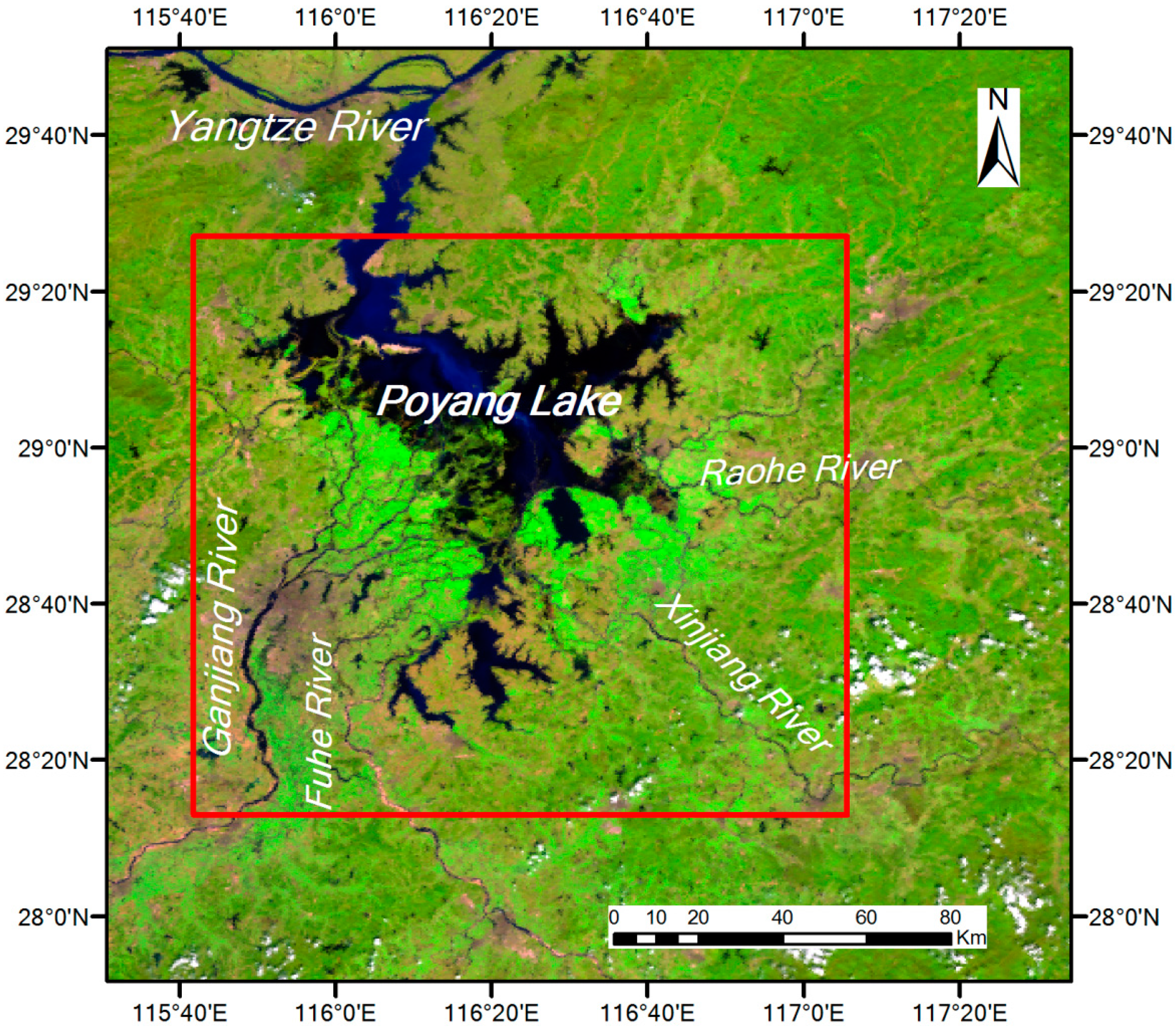
2.1. Study Area and Materials
2.1.1. Study Area
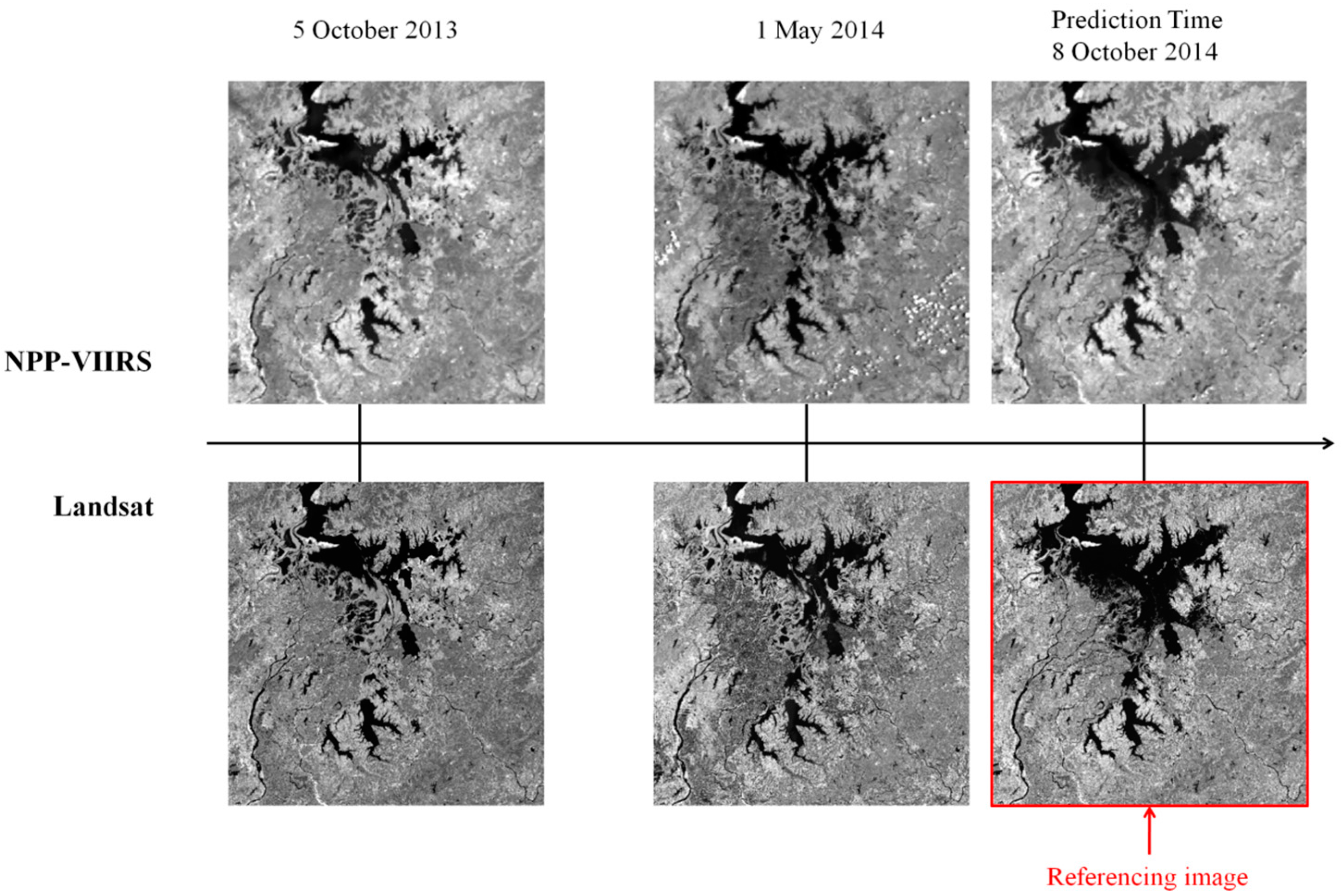
2.1.2. Materials
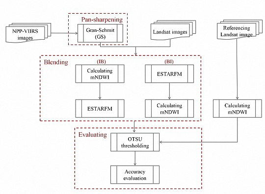
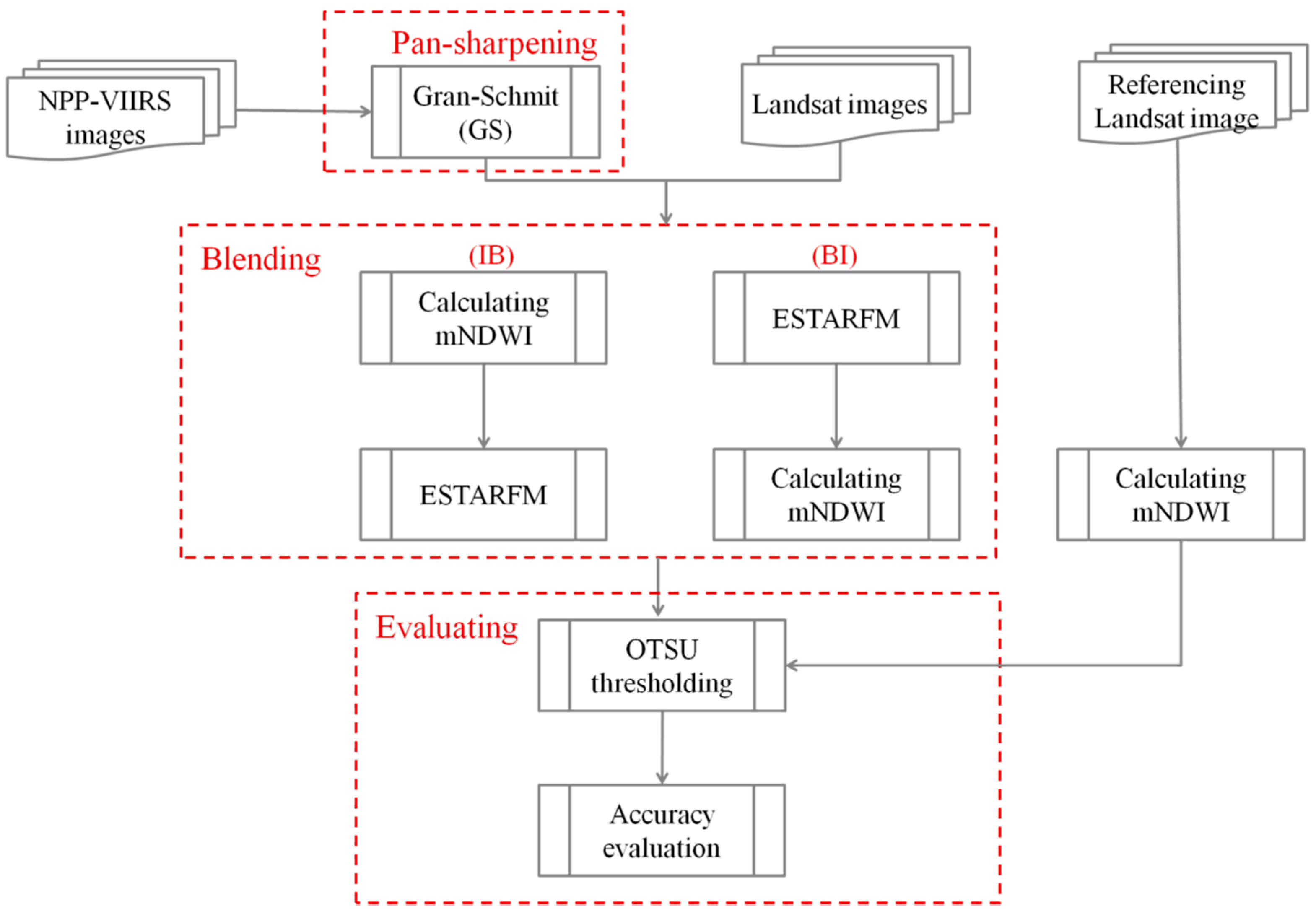
2.2. Methods
2.2.1. Pan-Sharpening of NPP-VIIRS
2.2.2. Blending NPP-VIIRS with Landsat OLI
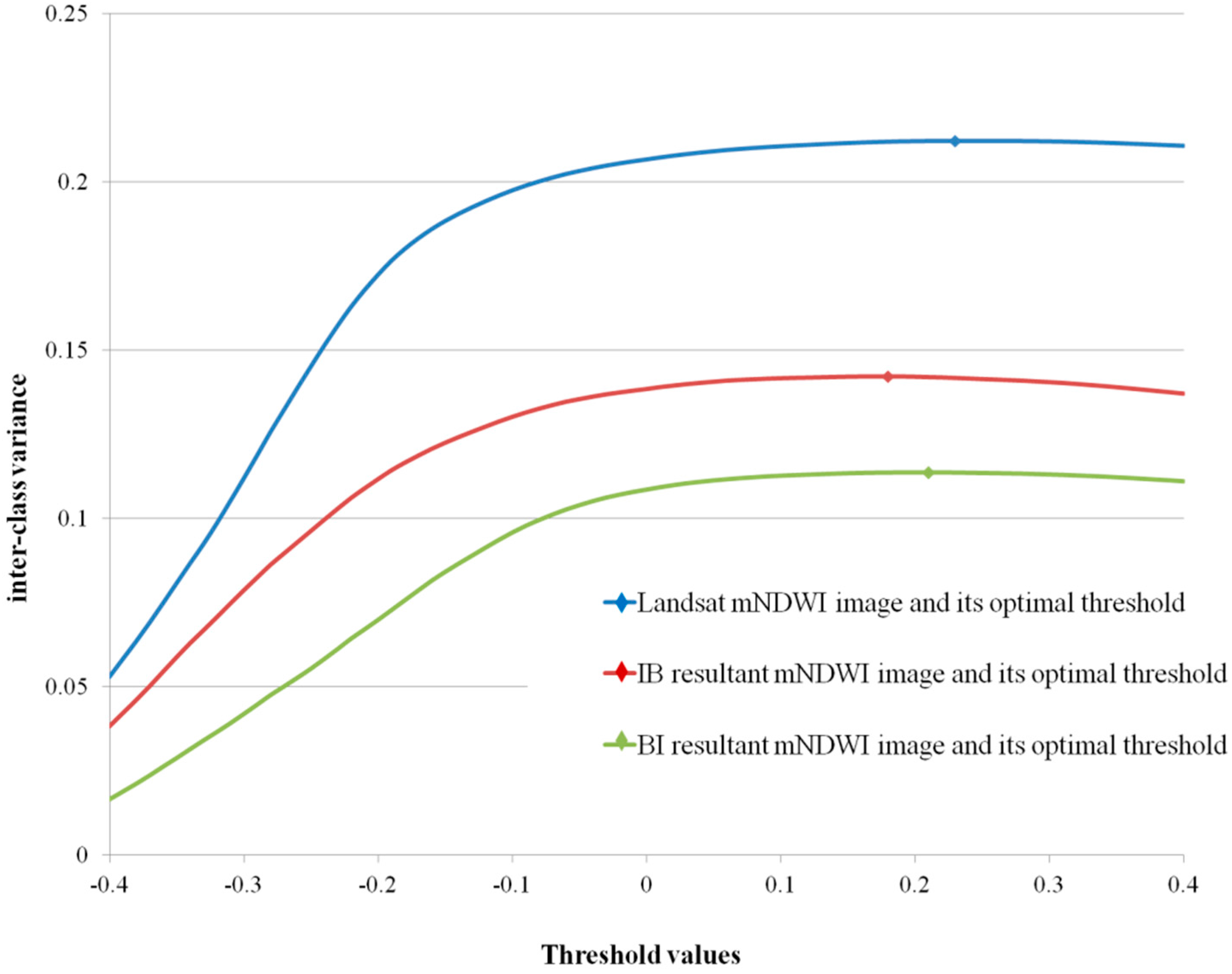
2.2.3. Evaluating the Accuracy of Blending Results
3. Results and Discussion
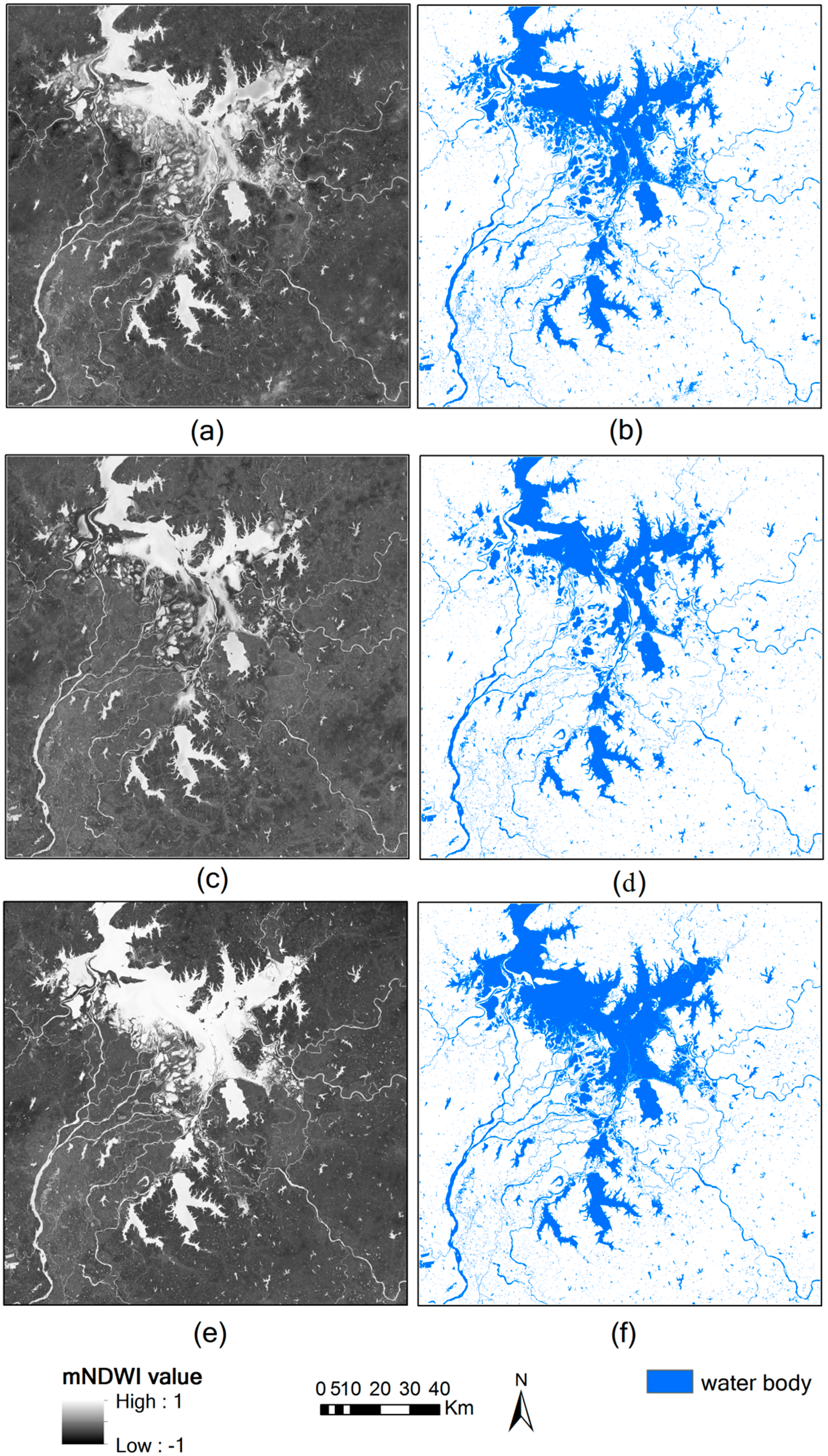
3.1. Blending Results
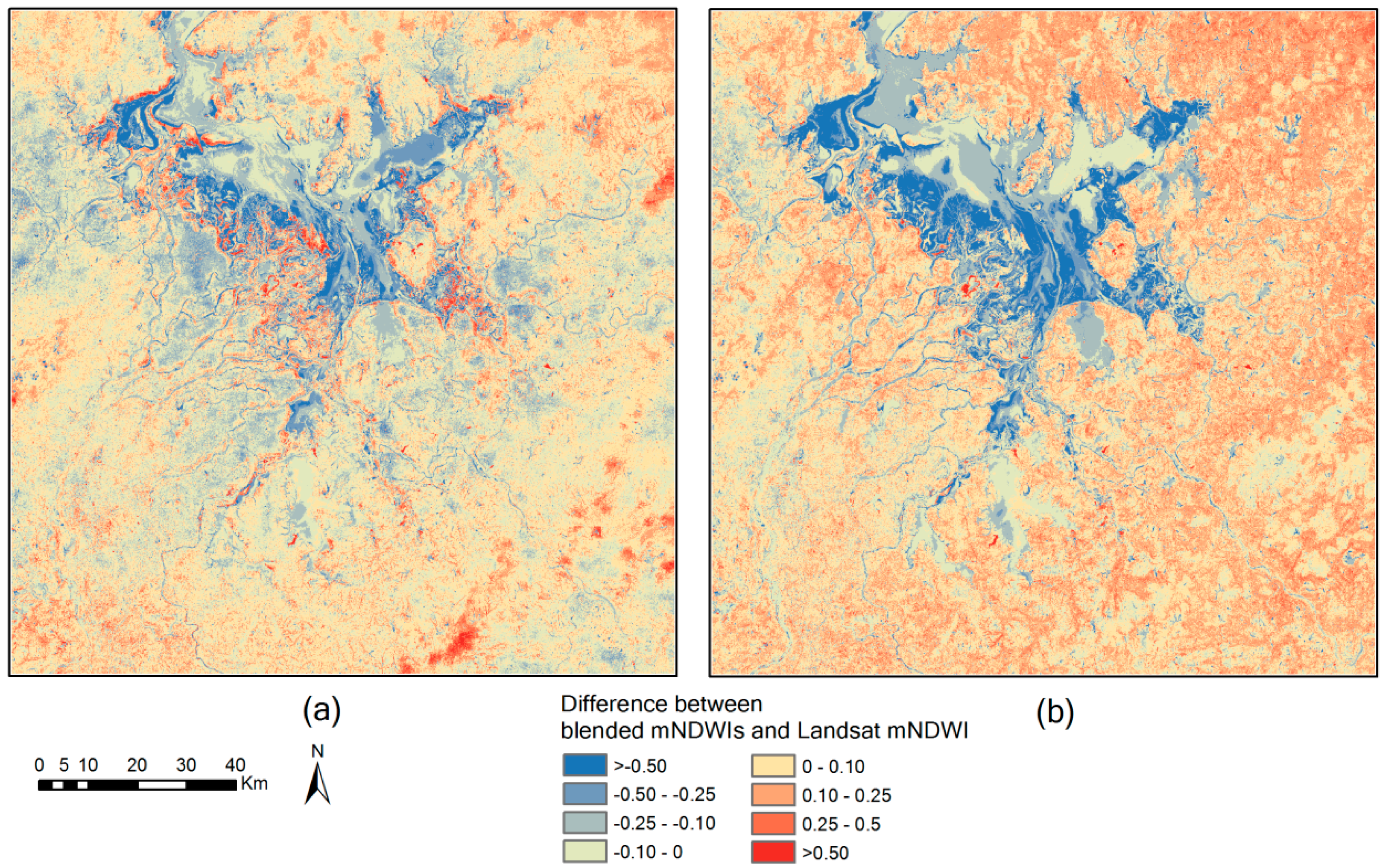
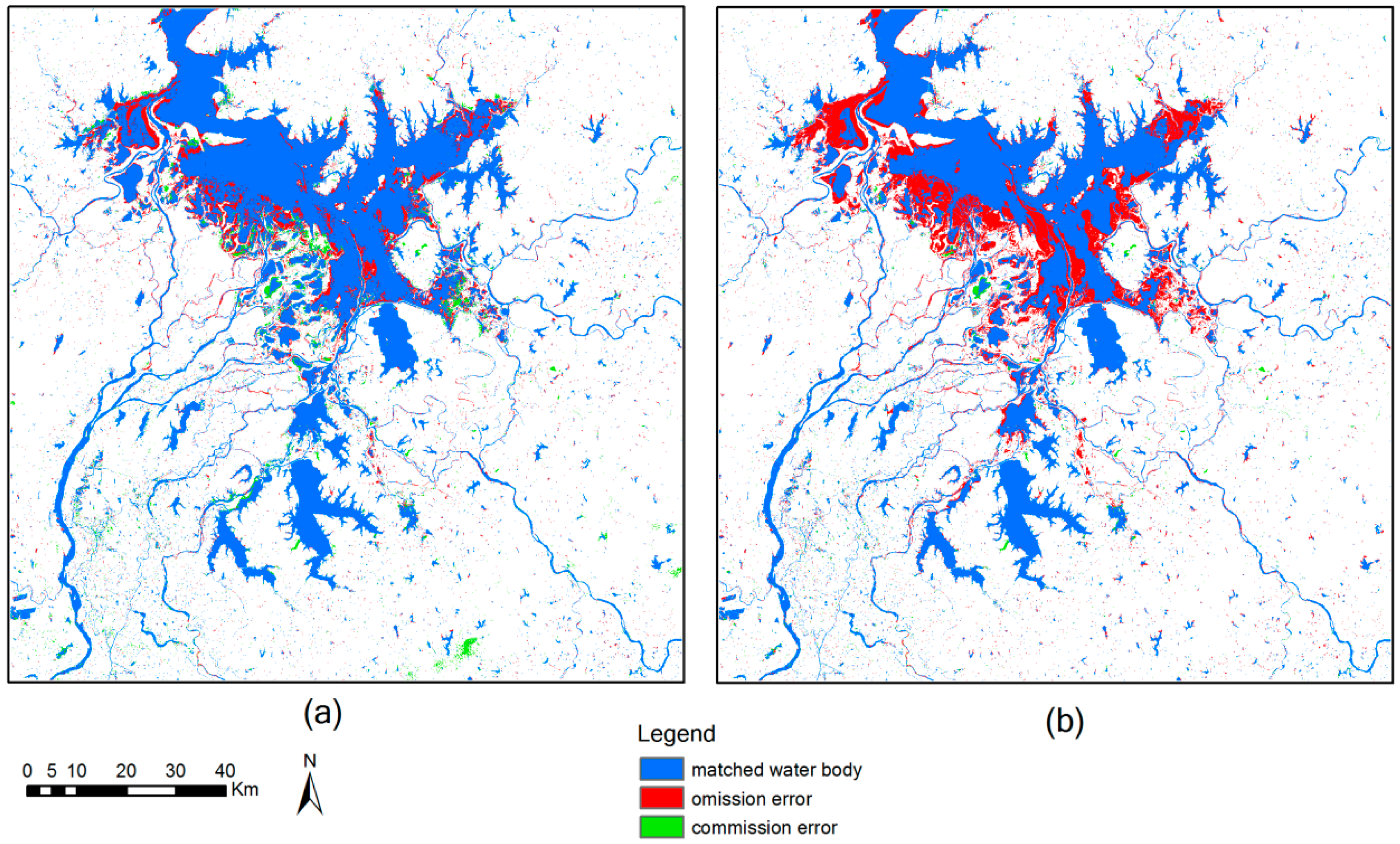
3.2. Comparison and Evaluation
4. Conclusions
Acknowledgments
Author Contributions
Conflicts of Interest
Abbreviations
| (Suomi) NPP-VIIRS | Visible Infrared Imaging Radiometer Suite onboard Suomi National Polar-orbiting Partnership |
| STARFM | Spatial and Temporal Adaptive Reflectance Fusion Model |
| ESTARFM | Enhanced Spatial and Temporal Adaptive Reflectance Fusion Model |
| mNDWI | modified Normalized Difference Water Index |
| BI | Blend-then-Index approach |
| IB | Index-then-Blend approach |
| MSS | Multispectral Sacnner |
| TM | Thematic Mapper |
| ETM+ | Enhanced Thematic Mapper Plus |
| OLI | Operational Land Imager |
| AVHRR | Advanced Very High Resolution Radiometer |
| MODIS | Moderate Resolution Imaging Spectroradiometer |
| NIR | Near Infrared |
| SWIR | Short-wave Infrared |
| GS | Gram-Schmidt |
| MS | Multispectral |
References
- Rango, A.; Salomonson, V.V. Regional flood mapping from space. Water Resour. Res. 1974, 10, 473–484. [Google Scholar] [CrossRef]
- Chen, Y.; Wang, B.; Pollino, C.A.; Cuddy, S.M.; Merrin, L.E.; Huang, C. Estimate of flood inundation and retention on wetlands using remote sensing and GIS. Ecohydrology 2014, 7, 1412–1420. [Google Scholar] [CrossRef]
- Feyisa, G.L.; Meilby, H.; Fensholt, R.; Proud, S.R. Automated Water Extraction Index: A new technique for surface water mapping using Landsat imagery. Remote Sens. Environ. 2014, 140, 23–35. [Google Scholar] [CrossRef]
- Zhang, G.; Yao, T.; Xie, H.; Zhang, K.; Zhu, F. Lakes’ state and abundance across the Tibetan Plateau. Chin. Sci. Bull. 2014, 59, 3010–3021. [Google Scholar] [CrossRef]
- Li, J.; Sheng, Y. An automated scheme for glacial lake dynamics mapping using Landsat imagery and digital elevation models: A case study in the Himalayas. Int. J. Remote Sens. 2012, 33, 5194–5213. [Google Scholar] [CrossRef]
- Li, W.; Du, Z.; Ling, F.; Zhou, D.; Wang, H.; Gui, Y.; Sun, B.; Zhang, X. A Comparison of Land surface water mapping using the normalized difference water index from TM, ETM+ and ALI. Remote Sens. 2013, 5, 5530–5549. [Google Scholar] [CrossRef]
- Barton, I.J.; Bathols, J.M. Monitoring floods with AVHRR. Remote Sens. Environ. 1989, 30, 89–94. [Google Scholar] [CrossRef]
- Jain, S.K.; Saraf, A.K.; Goswami, A.; Ahmad, T. Flood inundation mapping using NOAA AVHRR data. Water Resour. Manag. 2006, 20, 949–959. [Google Scholar] [CrossRef]
- Chen, Y.; Huang, C.; Ticehurst, C.; Merrin, L.; Thew, P. An Evaluation of MODIS Daily and 8-day composite products for floodplain and wetland inundation mapping. Wetlands 2013, 33, 823–835. [Google Scholar] [CrossRef]
- Huang, C.; Chen, Y.; Wu, J. Mapping spatio-temporal flood inundation dynamics at large river basin scale using time-series flow data and MODIS imagery. Int. J. Appl. Earth Obs. Geoinform. 2014, 26, 350–362. [Google Scholar] [CrossRef]
- Liu, R.; Chen, Y.; Wu, J.; Gao, L.; Barrett, D.; Xu, T.; Li, L.; Huang, C.; Yu, J. Assessing spatial likelihood of flooding hazard using naïve Bayes and GIS: A case study in Bowen Basin, Australia. Stoch. Environ. Res. Risk Assess. 2015, 30, 1575–1590. [Google Scholar] [CrossRef]
- Du, Z.; Li, W.; Zhou, D.; Tian, L.; Ling, F.; Wang, H.; Gui, Y.; Sun, B. Analysis of Landsat-8 OLI imagery for land surface water mapping. Remote Sens. Lett. 2014, 5, 672–681. [Google Scholar] [CrossRef]
- Shi, K.; Huang, C.; Yu, B.; Yin, B.; Huang, Y.; Wu, J. Evaluation of NPP-VIIRS night-time light composite data for extracting built-up urban areas. Remote Sens. Lett. 2014, 5, 358–366. [Google Scholar] [CrossRef]
- Yu, Y.; Privette, J.L.; Pinheiro, A.C. Analysis of the NPOESS VIIRS land surface temperature algorithm using MODIS data. IEEE Trans. Geosci. Remote Sens. 2005, 43, 2340–2350. [Google Scholar]
- Huang, C.; Chen, Y.; Wu, J.; Li, L.; Liu, R. An evaluation of suomi NPP-VIIRS data for surface water detection. Remote Sens. Lett. 2015, 6, 155–164. [Google Scholar] [CrossRef]
- Huang, C.; Chen, Y.; Wu, J.P. DEM-based modification of pixel-swapping algorithm for enhancing floodplain inundation mapping. Int. J. Remote Sens. 2014, 35, 365–381. [Google Scholar] [CrossRef]
- Li, L.; Chen, Y.; Xu, T.; Liu, R.; Shi, K.; Huang, C. Super-resolution mapping of wetland inundation from remote sensing imagery based on integration of back-propagation neural network and genetic algorithm. Remote Sens. Environ. 2015, 164, 142–154. [Google Scholar] [CrossRef]
- Li, L.; Chen, Y.; Yu, X.; Liu, R.; Huang, C. Sub-pixel flood inundation mapping from multispectral remotely sensed images based on discrete particle swarm optimization. ISPRS J. Photogramm. Remote Sens. 2015, 101, 10–21. [Google Scholar] [CrossRef]
- Pohl, C.; van Genderen, J.L. Review article Multisensor image fusion in remote sensing: Concepts, methods and applications. Int. J. Remote Sens. 1998, 19, 823–854. [Google Scholar] [CrossRef]
- Huang, B.; Zhang, H.; Song, H.; Wang, J.; Song, C. Unified Fusion of Remote-Sensing Imagery: Generating Simultaneously High-Resolution Synthetic Spatial-Temporal-Spectral Earth Observations. Remote Sens. Lett. 2013, 4, 561–569. [Google Scholar] [CrossRef]
- Zhang, L.; Shen, H.; Gong, W.; Zhang, H. Adjustable model-based fusion method for multispectral and panchromatic images. IEEE Trans. Syst. Man Cybern. B Cybern. A Publ. IEEE Syst. Man Cybern. Soc. 2012, 42, 1693–1704. [Google Scholar] [CrossRef] [PubMed]
- Yuan, Q.; Zhang, L.; Shen, H. Hyperspectral Image Denoising Employing a Spectral-Spatial Adaptive Total Variation Model. IEEE Trans. Geosci. Remote Sens. 2012, 50, 3660–3677. [Google Scholar] [CrossRef]
- Wu, P.; Shen, H.; Zhang, L.; Göttsche, F.M. Integrated fusion of multi-scale polar-orbiting and geostationary satellite observations for the mapping of high spatial and temporal resolution land surface temperature. Remote Sens. Environ. 2015, 156, 169–181. [Google Scholar] [CrossRef]
- Gao, F.; Masek, J.; Schwaller, M.; Hall, F. On the blending of the Landsat and MODIS surface reflectance: Predicting daily Landsat surface reflectance. IEEE Trans. Geosci. Remote Sens. 2006, 44, 2207–2218. [Google Scholar]
- Zhu, X.; Chen, J.; Gao, F.; Chen, X.; Masek, J.G. An enhanced spatial and temporal adaptive reflectance fusion model for complex heterogeneous regions. Remote Sens. Environ. 2010, 114, 2610–2623. [Google Scholar] [CrossRef]
- Chen, B.; Ge, Q.; Fu, D.; Yu, G.; Sun, X.; Wang, S.; Wang, H. A data-model fusion approach for upscaling gross ecosystem productivity to the landscape scale based on remote sensing and flux footprint modelling. Biogeosciences 2010, 7, 2943–2958. [Google Scholar] [CrossRef]
- Gaulton, R.; Hilker, T.; Wulder, M.A.; Coops, N.C.; Stenhouse, G. Characterizing stand-replacing disturbance in western Alberta grizzly bear habitat, using a satellite-derived high temporal and spatial resolution change sequence. For. Ecol. Manag. 2011, 261, 865–877. [Google Scholar] [CrossRef]
- Liu, H.; Weng, Q. Enhancing temporal resolution of satellite imagery for public health studies: A case study of West Nile Virus outbreak in Los Angeles in 2007. Remote Sens. Environ. 2012, 117, 57–71. [Google Scholar] [CrossRef]
- Zhang, F.; Zhu, X.; Liu, D. Blending MODIS and Landsat images for urban flood mapping. Int. J. Remote Sens. 2014, 35, 3237–3253. [Google Scholar] [CrossRef]
- Chen, B.; Huang, B.; Xu, B. Fine Land Cover Classification Using Daily Synthetic Landsat-Like Images at 15-m Resolution. IEEE Geosci. Remote Sens. Lett. 2015, 12, 2359–2363. [Google Scholar] [CrossRef]
- Hazaymeh, K.; Hassan, Q.K. Spatiotemporal image-fusion model for enhancing the temporal resolution of Landsat-8 surface reflectance images using MODIS images. J. Appl. Remote Sens. 2015, 9. [Google Scholar] [CrossRef]
- Weng, Q.; Gao, F.; Fu, P. Generating daily land surface temperature at Landsat resolution by fusing Landsat and MODIS data. Remote Sens. Environ. 2014, 145, 55–67. [Google Scholar] [CrossRef]
- Jarihani, A.A.; McVicar, T.R.; Van Niel, T.G.; Emelyanova, I.V.; Callow, J.N.; Johansen, K. Blending Landsat and MODIS Data to Generate Multispectral Indices: A Comparison of “Index-then-Blend” and “Blend-then-Index” Approaches. Remote Sens. 2014, 6, 9213–9238. [Google Scholar] [CrossRef] [Green Version]
- Xu, H.Q. Modification of normalised difference water index (NDWI) to enhance open water features in remotely sensed imagery. Int. J. Remote Sens. 2006, 27, 3025–3033. [Google Scholar] [CrossRef]
- Du, Y.; Zhang, Y.; Ling, F.; Wang, Q.; Li, W.; Li, X. Water Bodies’ Mapping from Sentinel-2 Imagery with Modified Normalized Difference Water Index at 10-m Spatial Resolution Produced by Sharpening the SWIR Band. Remote Sens. 2016, 8, 354–370. [Google Scholar] [CrossRef] [Green Version]
- Shankman, D.; Liang, Q. Landscape Changes and Increasing Flood Frequency in China’s Poyang Lake Region. Prof. Geogr. 2003, 55, 434–445. [Google Scholar] [CrossRef]
- Xu, G.; Qin, Z. Flood Estimation Methods for Poyang Lake Area. J. Lake Sci. 1998, 10, 31–36. [Google Scholar]
- Shankman, D.; Keim, B.D.; Song, J. Flood frequency in China’s Poyang Lake Region: Trends and teleconnections. Int. J. Climatol. 2006, 26, 1255–1266. [Google Scholar] [CrossRef]
- Feng, L.; Hu, C.M.; Chen, X.L.; Cai, X.B.; Tian, L.Q.; Gan, W.X. Assessment of inundation changes of Poyang Lake using MODIS observations between 2000 and 2010. Remote Sens. Environ. 2012, 121, 80–92. [Google Scholar] [CrossRef]
- Aiazzi, B.; Baronti, S.; Selva, M.; Alparone, L. Enhanced Gram-Schmidt Spectral Sharpening Based on Multivariate Regression of MS and Pan Data. In Proceedings of the IEEE International Conference on Geoscience and Remote Sensing, Denver, CO, USA, 31 July–4 August 2006.
- Kneusel, R.T.; Kneusel, P.N. Novel PET/CT Image Fusion via Gram-Schmidt Spectral Sharpening. In Proceedings of the SPIE—Medical Imaging 2013: Image Processing, Lake Buena Vista, FL, USA, 9 February 2013.
- McFeeters, S.K. The use of the normalized difference water index (NDWI) in the delineation of open water features. Int. J. Remote Sens. 1996, 17, 1425–1432. [Google Scholar] [CrossRef]
- Otsu, N. A Threshold Selection Method from Gray-Level Histograms. IEEE Trans. Syst. Man Cybern. 1979, 9, 62–66. [Google Scholar]


| Spectral Region | Landsat OLI Band | Landsat OLI Wavelength (μm) | NPP-VIIRS Band | NPP-VIIRS Wavelength (μm) | Landsat OLI Pixel Size (m) | NPP-VIIRS Pixel Size (m) |
|---|---|---|---|---|---|---|
| Coastal | 1 | 0.433–0.453 | M2 | 0.436−0.454 | 30 | 750 |
| Blue | 2 | 0.450–0.515 | M3 | 0.478–0.488 | 30 | 750 |
| * Green | 3 | 0.525–0.600 | M4 | 0.545–0.565 | 30 | 750 |
| Red | 4 | 0.630–0.680 | M5/I1 | 0.662–0.682/0.600–0.680 | 30 | 750/375 |
| NIR | 5 | 0.845–0.885 | M7/I2 | 0.846–0.885/0.850–0.880 | 30 | 750/375 |
| * SWIR1 | 6 | 1.560–1.660 | M10/I3 | 1.580–1.640/1.580–1.640 | 30 | 750/375 |
| SWIR2 | 7 | 2.100–2.300 | M11 | 2.230–2.280 | 30 | 750 |
| Pan | 8 | 0.5000–0.680 | -- | -- | 15 | -- |
| Cirrus | 9 | 1.360–1.390 | M9 | 1.371–1.386 | 30 | 750 |
| Blending Approach | Omission Error (%) | Commission Error (%) | Overall Accuracy (%) | Kappa Coefficient |
|---|---|---|---|---|
| IB | 2.72 | 1.02 | 96.26 | 0.87 |
| BI | 5.04 | 0.39 | 94.57 | 0.80 |
© 2016 by the authors; licensee MDPI, Basel, Switzerland. This article is an open access article distributed under the terms and conditions of the Creative Commons Attribution (CC-BY) license (http://creativecommons.org/licenses/by/4.0/).
Share and Cite
Huang, C.; Chen, Y.; Zhang, S.; Li, L.; Shi, K.; Liu, R. Surface Water Mapping from Suomi NPP-VIIRS Imagery at 30 m Resolution via Blending with Landsat Data. Remote Sens. 2016, 8, 631. https://doi.org/10.3390/rs8080631
Huang C, Chen Y, Zhang S, Li L, Shi K, Liu R. Surface Water Mapping from Suomi NPP-VIIRS Imagery at 30 m Resolution via Blending with Landsat Data. Remote Sensing. 2016; 8(8):631. https://doi.org/10.3390/rs8080631
Chicago/Turabian StyleHuang, Chang, Yun Chen, Shiqiang Zhang, Linyi Li, Kaifang Shi, and Rui Liu. 2016. "Surface Water Mapping from Suomi NPP-VIIRS Imagery at 30 m Resolution via Blending with Landsat Data" Remote Sensing 8, no. 8: 631. https://doi.org/10.3390/rs8080631