Quantifying Snow Cover Distribution in Semiarid Regions Combining Satellite and Terrestrial Imagery

1
Fluvial Dynamics and Hydrology Research Group, Andalusian Institute for Earth System Research, University of Córdoba, Campus Rabanales, Edificio Leonardo da Vinci, Área de Ingeniería Hidráulica, 14017 Córdoba, Spain
2
Hydrology Research Unit, Swedish Meteorological and Hydrological Institute, Folkborgsvägen 17, 601 76 Norrköping, Sweden
*
Author to whom correspondence should be addressed.
Remote Sens. 2017, 9(10), 995; https://doi.org/10.3390/rs9100995
Submission received: 29 August 2017
/
Revised: 15 September 2017
/
Accepted: 22 September 2017
/
Published: 26 September 2017
(This article belongs to the Special Issue Snow Remote Sensing)
Abstract
:Mediterranean mountainous regions constitute a climate change hotspot where snow plays a crucial role in water resources. The characteristic snow-patched distribution over these areas makes spatial resolution the limiting factor for its correct representation. This work assesses the estimation of snow cover area and the contribution of the patchy areas to the seasonal and annual regime of the snow in a semiarid mountainous range, the Sierra Nevada Mountains in southern Spain, by means of Landsat imagery combined with terrestrial photography (TP). Two methodologies were tested: (1) difference indexes to produce binary maps; and (2) spectral mixture analysis (SMA) to obtain fractional maps; their results were validated from “ground-truth” data by means of TP in a small monitored control area. Both methods provided satisfactory results when the snow cover was above 85% of the study area; below this threshold, the use of spectral mixture analysis is clearly recommended. Mixed pixels can reach up to 40% of the area during wet and cold years, their importance being larger as altitude increases, proving the usefulness of TP for assessing the accuracy of remote data sources. Mixed pixels identification allows for determining the more vulnerable areas facing potential changes of the snow regime due to global warming and climate variability.
1. Introduction
In general, snowmelt-dominant regions are located in latitudes greater than 45° (North and South). Intense efforts to study snow dynamics have been developed over these areas, in which a continuous and deep snowpack can be usually found throughout large areas. However, there are many mountainous regions located in lower and warmer latitudes, which are highly dependent of snow water resources for agriculture and water supply, despite snow occurrence being non-uniform and highly timing during the cold season. Over these areas, climate change effects are likely to be more noticeable and, thus, they constitute a natural laboratory for their early detection and evaluation [1,2]. This is the case of semiarid mountainous regions, where high level of income solar radiation, mild winters, and torrential precipitation regimes are usual intrinsic features of their climate [3,4]; water scarcity and drought periods are found to be currently increasing, as many authors have stated [5,6,7]. In these regions, snow does not follow a single and somehow continuous accumulation-snowmelt cycle, more commonly found in colder regions, being the spring season representative of a significant inflow of melting water to the surface and groundwater bodies. A typical semiarid snowpack exhibits a very strong spatiotemporal variability, and very often undergoes different accumulation-snowmelt cycles during the cold season in a given year. The ablation process usually results in patched distribution of snow around local singularities, such as rocks, vegetation bunches, depressions, among others [8,9,10]. These snow patches evolve into a mosaic-type spatial pattern with alternating snow-covered and snow-free areas, whose size ranges between one to dozens of square meters. Their local spatial evolution is governed by two main drivers: microscale patterns (~1 m) conditioned by the interaction between the snow and the micro-topography [8] and medium-sized patterns (~100 m) highly influenced by wind, and terrain curvature [11].
In recent decades, remote sensing has been providing distributed information about the snowpack all over the world and it is the major method for monitoring snow at medium–large scales, complementing the traditional in situ field surveys and ground automatic measurements to cover large areas. Snow cover fraction (SCF), snow albedo (SA), and snow water equivalent (SWE) are the most common variables measured by using both optical and radar remote sensing imagery, based, respectively, on the highly different brightness temperature between the visible and near-infrared regions [12,13,14,15] and on the signal attenuation due to the water present in the snowpack [16,17]. Among them, SCF is the most usually targeted information from which further variables are then derived, especially in distributed modeling of the snow processes [18,19].
Within the great amount of remote sensing information (e.g., NOAA, daily images with 1 km × 1 km cell size; MODIS, daily images with 500 × 500 m cell size; Landsat Thematic Mapper, 16-day images with 30 m × 30 m cell size), the selection of the dataset is closely related to the scale of the targeted processes. Spatial resolution is the limiting factor for the detection of snow in semiarid regions, since the extremely changing conditions favor a particularly snow distribution, which usually appears as medium-to-small sized patches [20,21]. Hence, those datasets with a higher spatial resolution, such as Landsat Thematic Mapper (TM) and Enhanced Thematic Mapper (ETM+) data, are recommended in these studies [22,23,24], since, for example, MODIS snow products, with a 500 × 500 m spatial resolution, are not capable to capture the significant sub-grid distribution currently found. Another alternative for the study of the snow extension over these changeable areas is the use of terrestrial photography (TP), that is, images taken from the Earth surface and whose spatial and temporal resolution can be adapted to the study problem [8,9,18,25,26]. Despite the advantages of this technique, easy adaptation to the temporal and spatial resolution of the studied processes under monitoring, its use over large and abrupt mountainous areas is limited since, on one hand, a great number of images would be required, and, on the other hand, there is some lack of information associated with the non-visible areas, which can be significant in some cases.
However, the combination of both data sources may overcome their individual scale-related limitations provided that a long-time series is available. For this, the high-resolution TP images over a given area can be assumed as the ground-truth information associated to the snow cover area distribution, against which snow detection algorithms to be applied to the lower resolution satellite images, such as Landsat TM and ETM+.
The traditional classification algorithms for snow detection are based on normalized indexes which provide a binary classification as snow and no-snow pixels throughout the study area [15,27]; this simple classification may result in large error in heterogeneous and transitional areas within the snow-dominated domain [14]. Alternatively, the spectral mixture analysis (SMA) approach provides fraction of snow cover within each pixel and thus, constitutes a step forward to characterize heterogeneous and patchy snow areas in semiarid regions. This method requires an external dataset, with higher spatial resolution, to calibrate and validate the algorithms used. In [28] calculated snow cover fraction values from MODIS (500 × 500 m2) using Landsat scenes (30 × 30 m2) as calibration and validation dataset in Sierra Nevada (USA), Rocky Mountains, high plains of Colorado and Himalaya, and obtained a mean relative error in the analyzed scenes of 5%, ranging from 1% to 13%. Nevertheless, the significant patch size scales of the snow distribution in Mediterranean regions require the use of Landsat imagery as primary source when the evolution of this patchy snowpack is the targeted goal on the mid and long term.
This work assesses the estimation of snow cover area in semiarid regions during different stages in the snow season by means of Landsat imagery and the contribution of the patchy areas in these regions to the seasonal and annual regime of the snow. For this, a 14-year series of snow cover maps (30 × 30 m) was obtained from Landsat imagery in the Sierra Nevada Mountains in southern Spain. Two methodologies were tested for the estimation of the SCF: (1) the use of difference indexes to obtain binary maps (covered and non-covered pixels); and (2) a spectral mixture analysis model to calculate fractional snow cover maps (fraction of coverage inside each pixel). The performance of both methodologies is assessed by means of SCF maps (10 × 10 m) obtained from TP in a small monitored control area in the study site.
2. Study Site and Available Data
This study is carried out in Sierra Nevada Mountains, Southern Spain (Figure 1A,B). They are a linear mountain range of 90-km length, that running parallel to the coastline of Mediterranean Sea, where the Alpine and Mediterranean climate conditions can be found in just a 40-km distance. Strong altitudinal gradients with marked differences between the south (directly affected to the sea) and the north faces are found in the area. Its high summits make snow the main factor that conditions most of the hydrological and ecological processes over the area. The particular characteristics make Sierra Nevada a rich reservoir of endemic wildlife species. It is considered the most important center of biodiversity in the western Mediterranean region, with over 2100 different vascular plant taxa recorded, accounting for nearly 30% of the vascular flora of the entire Iberian Peninsula [29,30]. The region is also environmentally protected, the highest elevations of the range were declared a part of a UNESCO Biosphere Reserve in 1986, a Natural Park in 1989, and a National Park in 1999.
The snow usually appears above 2000 m a.s.l. during winter and spring even though the snowmelt season generally lasts from April to June. The typically mild Mediterranean winters produce several snowmelt cycles before the final melting phase, which distributes the snow in patches over the terrain. Precipitation is heterogeneously distributed over the area because of the steep orography, with a high annual variability (400–1500 mm). The average temperature during the snow season can range from −5 °C to 5 °C, reaching values as low as −20 °C at certain times and location during winter [31]. Table 1 shows some statistical descriptors of the most relevant meteorological variables on an annual basis.
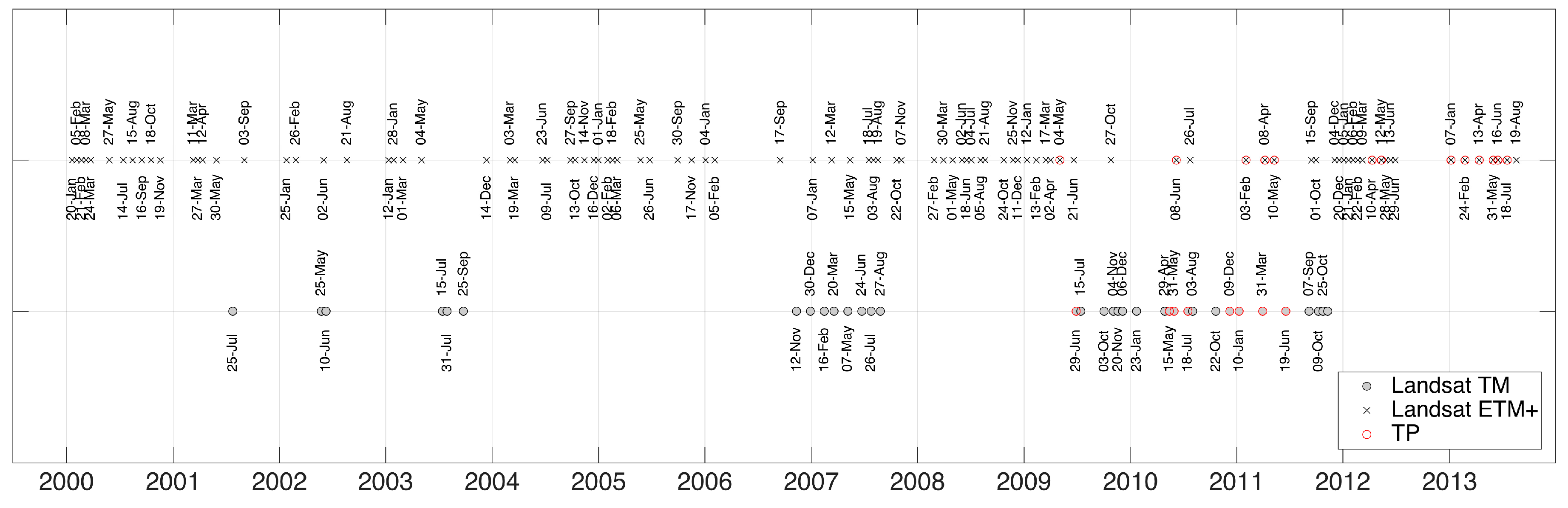
For this study, a total number of 132 Landsat TM and ETM+ scenes (temporal resolution of 16 days; spatial resolution of 30 × 30 m) were selected during the period (2000–2013) from the available cloud-free scenes (Table 2) to obtain 30 × 30 m snow cover maps of the study area by two different algorithms. Additionally, the available daily series of TP taken with a conventional digital camera from 2009 to 2013 covering an approximately 2-km2 control area, located in the western part of Sierra Nevada Mountains (Figure 1C) were used to extract a sub-set of images on the selected Landsat dates (Figure 2) from which validation of the resulting snow cover maps. This control area comprises a flat hillslope facing west with altitudes ranging from 1900 to 3011 m a.s.l. (the Caballo peak).
3. Methods
Binary and fractional snow cover maps were derived, respectively, from (1) normalized difference indexes analysis and (2) spectral mixture analysis for each one of the selected Landsat scenes showed in Figure 2. These images were pre-processed following the standard methods used in this area by Pimentel et al. (2012) [24].
3.1. Landsat Pre-Processing
The different stages in this pre-processing include a radiometric calibration, and atmospheric, saturation and topographic corrections. Angular correction is not applied since the surface is considered Lambertian. Although in reality snow surface is not Lambertian, this assumption does not introduce significant errors when the remote sensors are nadir viewing with a fixed direction. This is the case of TM and ETM+ sensor, which are nadir viewing and have an fixed incident, approximately 30°, being the anisotropy coefficient close to 1 [32,33,34].
The radiometric coefficients summarized in [35] were applied for the radiometric calibration. The atmospheric correction was performed by the Dark Object Subtraction (DOS) method used in many similar analyses [36,37]. This method retrieves the surface reflectance by assuming a Lambertian surface and cloudless atmospheric conditions, and it considers all the scattering effects in the scene to be the same as those of a blackbody present in the scene [38]; the dark object is selected from the minimum radiance value of the histogram made up from at least a 200-pixel sub-set in the scene [39] that must exclude those pixels shadowed by the terrain roughness. Moreover, fixed values for the downwelling transmittance parameters of the atmosphere for each band are adopted [40], being both the upwelling atmospheric transmittance and the diffuse irradiance neglected. DOS-based methods constitute a good alternative to the more complex Radiative Transference Codes (RTCs) when the atmospheric optical properties that they require are not fully available or have a questionable quality [41].
Several bands of Landsat scenes are radiometric-saturated due to the radiometric configuration of the sensors. Snow constitutes at most a 5% of the analyzed Landsat scenes and thus, the sensors are not specifically calibrated for snow, whatever the main land use is. This saturation is especially relevant during the winter, when the highest differences between the snow and the rest of land covers in the scene are found. To correct this saturation, a multivariable correlation analysis between bands is employed to recover the snow saturated pixels [42].
A C-correction algorithm [43] by means of a land cover separation [44] was applied as topographic correction to remove the effects of the terrain roughness on the image. Again, the Lambertian surface assumption allows the obtaining of a linear fit between the illumination angle and the different bands reflectance. Additionally, the diffuse irradiance is taken into account by a semi-empirical estimation of the C factor. In order to consider the multiple reflective properties of the different soil covers, the pixels are classified as bare soil or vegetated areas by using the Normalized Difference Vegetation Index (NDVI).
3.2. Snow Cover Maps
3.2.1. Binary Snow Cover Maps
The algorithm for deriving binary snow cover maps is based on the physical properties of a snow cover throughout the electromagnetic spectrum. Snow has very different extreme values in the visible (high reflectance) and infrared regions (low reflectance), so that a Normalized Difference Snow Index (NDSI) has been defined for each pixel over a threshold altitude (linked to the minimum height in which snow can be found) by comparing the individual electromagnetic responses in these two regions of a given pixel [45]. For Landsat TM and ETM+ scenes, the spectral bands that correspond with these two regions are band 2 (0.52–0.60 μm) and band 5 (1.55–1.75 μm). The index is defined as follows:
The discrimination between covered and non-covered pixels is done based on two threshold values: NDSI > 0.15 and band1 > 0.06 (0.45–0.52 μm), adopted to detect snow under the particular characteristics of snow in Mediterranean regions [46].
3.2.2. Fractional Snow Cover Maps from Spectral Mixture Analysis
This alternative algorithm provides an estimated value of the snow cover fraction (SCF) in each pixel, based on the assumption of the global reflectance of a mixed pixel (a pixel made up of different types of surfaces) being a linear combination of the individual reflectance values of the surfaces present in the pixel (endmembers). Thus, this endmembers-spectral mixture analysis (SMA) [21,47] expresses the reflectance in each pixel after the pre-processing, as the linear combination of the reflectance values from each spectral endmember given by Equation (2),
where is the fraction of the area of endmember i in a given pixel; is the reflectance of endmember at wavelength obtained after the pre-processing steps; N is the number of spectral endmembers taken into account; and is the residual error at the wavelength associated to the fit of the N endmembers considered in the analysis. The method requires, first, to select the significant endmembers in the study area and obtain their individual spectrum, and second, to solve the values for each pixel in the scene.
Three significant endmembers were identified in the study area: (a) pure snow, (b) vegetation (brush creeping vegetation) and (c) rocks (predominantly, phyllites). Their spectrums were obtained from a digital spectral library (http://speclab.cr.usgs.gov/) (Figure 3). The least-squares fit to is solved in each pixel with a reflective Newton method. The results from the SMA go beyond the discrimination of snow, since it allows identification of mixed pixels (when they occur and where they are located) and the study of their contribution to the snow cover area in the study site on different time scales.
3.2.3. Snow Cover Maps Validation
The results from both snow cover retrieval methods from Landsat TM and ETM+ were validated using the 10-m snow cover maps estimated from TP over the control area (Figure 1C) selected in the study area.
High Resolution Snow Cover Maps from Terrestrial Photography
Snow cover maps from TP are usually obtained in a two-step process [9]: (a) georeferencing and (b) snow detection. The first one is achieved following some basic principles of computing design [48,49] with the support of a Digital Elevation Model (DEM) of the target area. The result is a function that relates the two-dimensional elements (pixels) in the photo with the three-dimensional elements (points, centers of each cell) in the DEM [26]. The second step involves an unsupervised k-means algorithm that distinguishes between covered and non-covered pixels. The final result is a snow cover maps time series with the same spatial resolution of the DEM and the temporal resolution of the TP acquisition process. TP images can be a powerful data source that is easily adapted to the temporal and spatial resolution of the studied processes under monitoring.
Performance Indicators of the Snow Cover Map Algorithms
Virtual fractional 30 × 30 m2 snow maps are obtained from the binary 10 × 10 m2 snow maps resulting from the TP analysis, and they are used as “ground truth” to test the 30 × 30 m2 snow cover maps obtained from Landsat analysis by both algorithms, binary and spectral mixture approaches. The different metrics employed to evaluate the performance of each method [28] are given by Equations (3)–(6). Firstly, metrics to test the correct location of the pixels are used:
where RP represents the number of right positives (snow in both TP and Landsat pixels); RN represents the number of right negatives (no snow in both TP and Landsat pixels); WP represents the number of wrong positives (snow in the Landsat pixel and no-snow in the TP pixel); and WN represents the number of wrong negatives (no-snow in the Landsat Pixel and snow in the terrestrial pixel).
Finally, the Root Mean Square Error (RMSE) is also provided in the analysis of the SMA:
All these metrics are calculated for the area in each Landsat image associated to the mask calculated using TP over the control area (Figure 1C).
4. Results
This section shows the SCF evolution in the study area during the study period using both binary and fractional analysis. The results of the validation of both methodologies using TP at the control area are also described.
4.1. Snow Cover Map Series from Landsat Analysis
Figure 3 shows the average (Figure 3A) and standard deviation (Figure 3B) of the SCF during the study period in the study area (altitudes above 1500 m). SCF average and standard deviation follow parallel trends for both methodologies, with mean values of 0.13 m2 m−2 and 0.11 m2 m−2 for the average SCF, and 0.20 m2 m−2 and 0.23 m2 m−2 for the standard deviation, for the binary and fractional approaches, respectively. A general overestimation of the binary method can be observed, being higher during the accumulation phases, especially for heavy snowfall events that affect areas where snow in not usually found, which reaches areas where the snow is not usually present (e.g., 12 January 2003 and 6 March 2005 with differences between both methodologies about 0.1 m2 m−2). The threshold values used to discriminate the presence of snow were obtained in the southern face in the study area [46] ,with higher altitude predominance; this very likely overestimates the presence of snow on the whole domain of Sierra Nevada. These differences are smaller during the melting periods, in which the average SCF seems to be more equally represented by both methodologies. Nevertheless, the standard deviation over these periods (Figure 3B) shows a variable value, with a general overestimation of the binary maps, with a mean difference of 0.04 m2 m−2. Despite the observed overestimation, both methodologies produce similar average values during the study period that stem from different spatial distributions, whose mean and standard deviation values are shown in Figure 4.
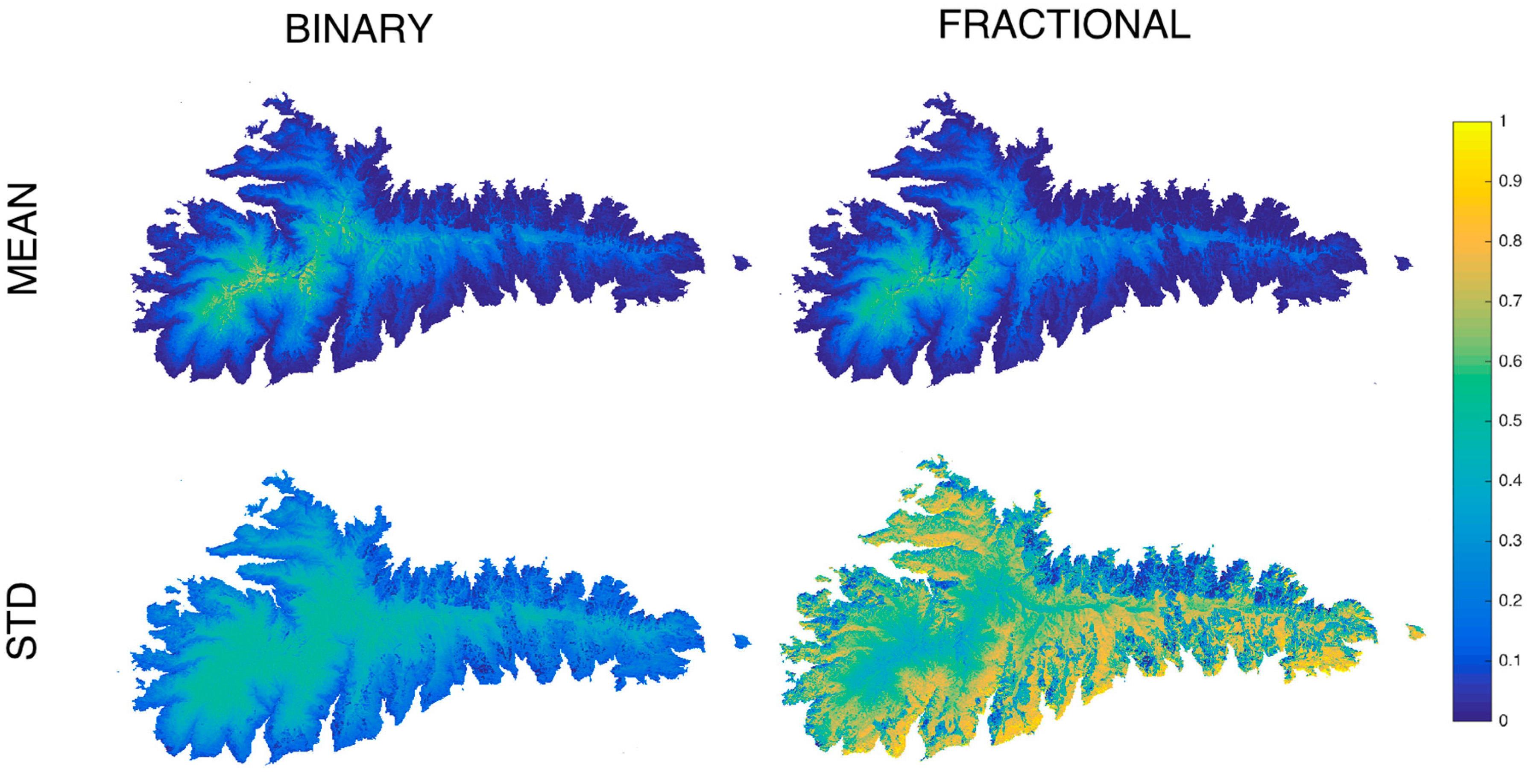
The local mean SCF value shows similar spatial patterns from both methodologies. In general, fractional maps present lower SCF values, being the higher differences between both approached found at the higher elevations located in the southwestern area, and at the lower elevations in the northeastern area; the binary methodology results in excess snow in the small valleys. On one hand, the first zone represents an area where the snow persistence is higher; consequently, longer melting cycles take place and there is a higher probability of occurrence of mixed pixels (pixels composed by snow and no snow). On the other hand, the second zone constitutes and area where the snow is very sporadic and associated to heavy snowfalls, which enhances the presence of mixed pixels, too. The local standard deviation distribution for the study period confirm this hypothesis, and shows a high spatial variability for the fractional method; it also provides a clear elevation fringe where the appearance of mixed pixels dominates the distribution of the snow in this mountainous range.
4.2. Snow Cover Map Validation from Terrestrial Photography
Landsat SCF maps were validated from the analysis of terrestrial pictures (assumed as “ground truth”) obtained over a control area (Figure 1C) during 2009–2013, following the method described in Section 3. Figure 5A shows three different examples of the SCF maps obtained from the three methods (binary and fractional algorithms, and terrestrial picture) for representative stages of the snow season: complete snow cover, beginning of the spring melting, and end of the melting cycle. The improvement in the snow cover detection is clearly observed from the left to the right of the figure (binary-fractional-TP), being the TP capable of capturing small patched patterns, which are commonly found in these mountain regions. Figure 5A also shows the loss of accuracy of the binary method as the melting period evolves. Three spatial distribution metrics are calculated to numerically validate the performance of the Landsat maps using as “ground truth” TP maps: precision, recall and accuracy (Figure 5B).
Precision describes the fraction of positive snow mapping results pixels that truly identified snow), that is, the ratio between the pixels detected as snow in Landsat and the snow pixels in TP. During the study period, its values range from 0.15 to 1, with a mean value of 0.75, for the binary maps, and from 0 to 1, with a mean value of 0.79, for the fractional maps. Similar precision values are obtained using both methodologies during the winter period, which is a slightly higher for the fractional maps. There is not a clear behavior of this metric during the melting period.
Recall describes the fraction of snow in all the scene that is identified by each method, that is, what fraction of the pixels detected as snow in TP are also detected by Landsat. It ranges from 0 to 1, with a mean value of 0.79, for the binary maps, and from 0.15 to 1, with a mean value of 0.86, in the case of the fractional maps. Recall values are again higher during the winter, but in this case the fractional maps shows better metric practically in all of the dates.
Finally, accuracy represents all the pixels correctly identified, whatever the situation is (snow or no-snow); so, this metric also takes into account the no-snow pixels. Accuracy ranges from 0.55 to 1, with a mean of 0.85, for the binary maps, and from 0.8 to 1, with a mean of 0.96, for the fractional maps. Fractional maps exhibit a clear better accuracy than binary maps, not only during winter but also during the melting periods. This is particularly relevant in regions where the persistence of the snowpack is not continuous, and different snow accumulation/melting cycles occur during a given season.
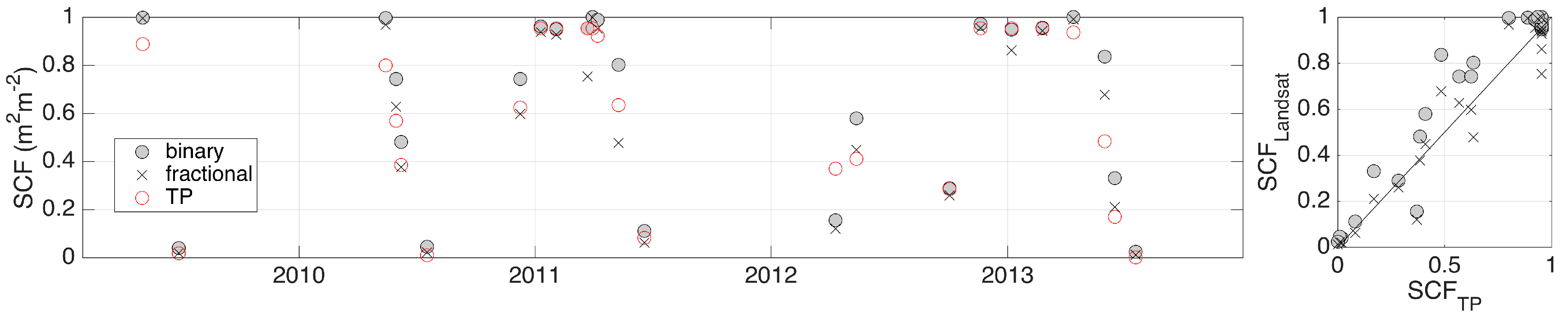
Figure 6 shows the evolution of the average SCF value over the control area from the Landsat maps and the validation TP dataset, together with the associated dispersion graph. Landsat binary and fractional maps present global RMSE values of 0.12 m2 m−2 and 0.09 m2 m−2, respectively, during the study period. Table 2 shows the absolute and relative error values for each Landsat map and date.
Generally, the fractional method results have a lower error than the binary, being this more relevant for snow cover area lower than 85% of the control area. The late melting stages obtain the worst representation, as expected, whatever algorithm is selected; however, the binary approach can produce large overestimations of the snow cover, which is not found with the fractional method.
4.3. Snow Cover Evolution from SMA Snow Maps
According to the previous results, the SMA method provides a better spatial representation of the snow throughout the study area. Moreover, the quick changes in the snowpack usually found in these latitudes are adequately represented by the resulting mixed pixels, with a realistic evolution of the snow captured by the sequence of fractional maps.
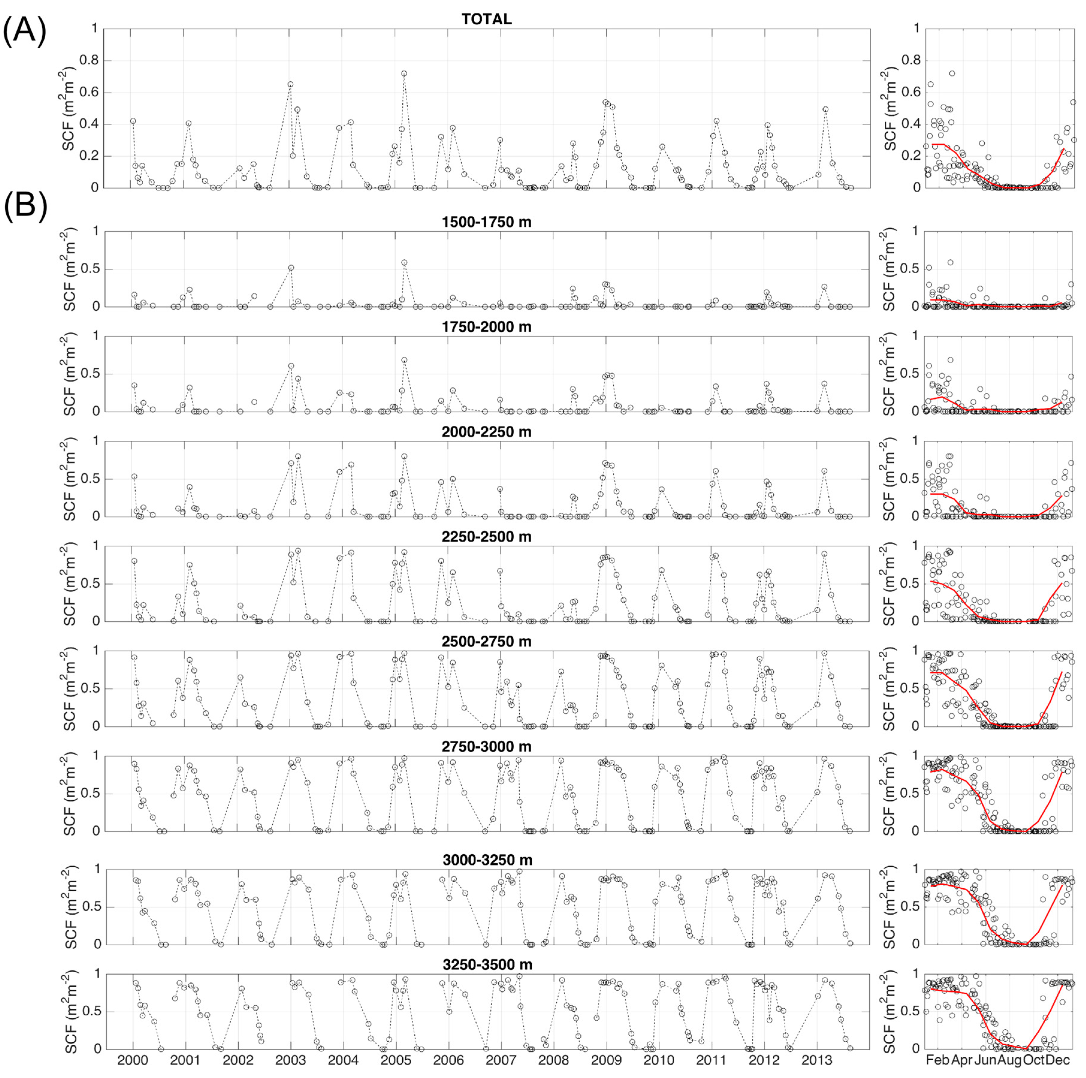
Figure 7 represents the evolution of the average SCF for different elevation bands over the Sierra Nevada mountainous range using fractional maps. The relationship between SCF and elevation at the study area can be assessed, both locally and globally, from these results. Below 1750 m a.s.l., snow very rarely approaches an average SCF value of 0.5; between 1750–2250 m a.s.l., SCF values are higher but never reach the complete cover of the area. 2250 m a.s.l. is estimated as the threshold elevation for which SCF equal or very close to 1 are found every year, with snow persistence increasing with altitude; the influence of high slopes that conditions the snow accumulation stability in the highest bands, especially when complete cover is reached, can also be observed from the results, proving the SMA approach to be capable of capturing these local conditions.
Figure 7 also identifies a threshold elevation band (2750–3000) above which the annual SCF pattern follows a clear accumulation phase during autumn, a consolidation period in winter, and a melting period during spring; values different to zero can be found every year, too. The duration of these phases and their evolution rate change depending on the elevation band, following the expected pattern: at higher elevations, the accumulation phase starts earlier and it evolves faster; snow consolidation is longer and melting is slow, which leaves remaining isolated snow-patched areas even during the summer. Below 2750 m a.s.l., there is not a distinct seasonal evolution of the snow pack, except for the absence of snow every summer; rather, a highly variable range of SCF values can be found during all the snow season, from autumn to spring.
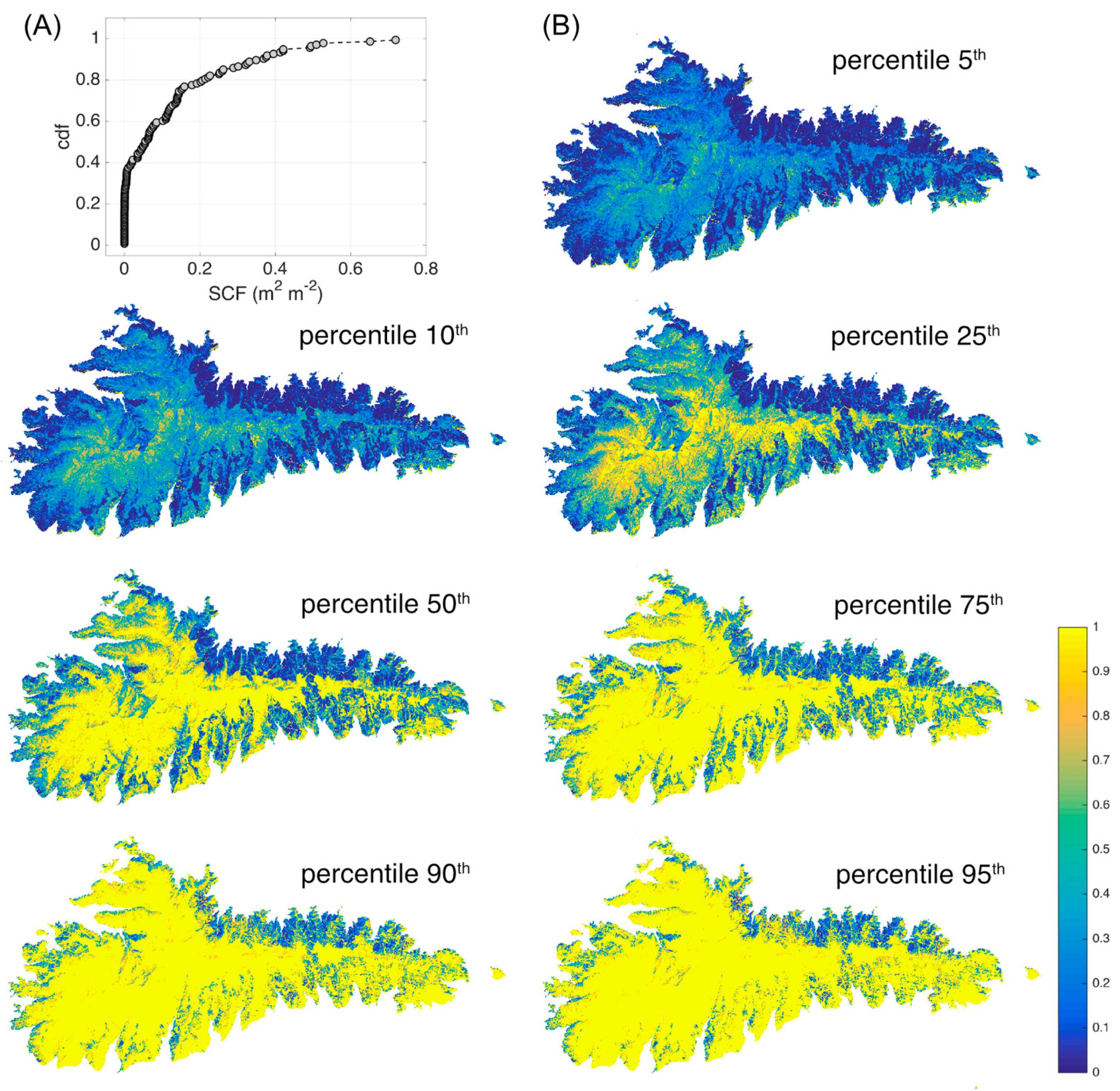
Figure 8 shows the cumulative distribution function (cdf) of the average SCF in the study area for the 2000–2013 period, together with the spatial distribution of selected percentiles of the pixel-SCF cdfs. The areas with less occurrence or persistence of snow can be easily identified at the surrounding of 1500 m a.s.l., especially in the northeastern area, together with the snow domain, mainly located in the upper areas.
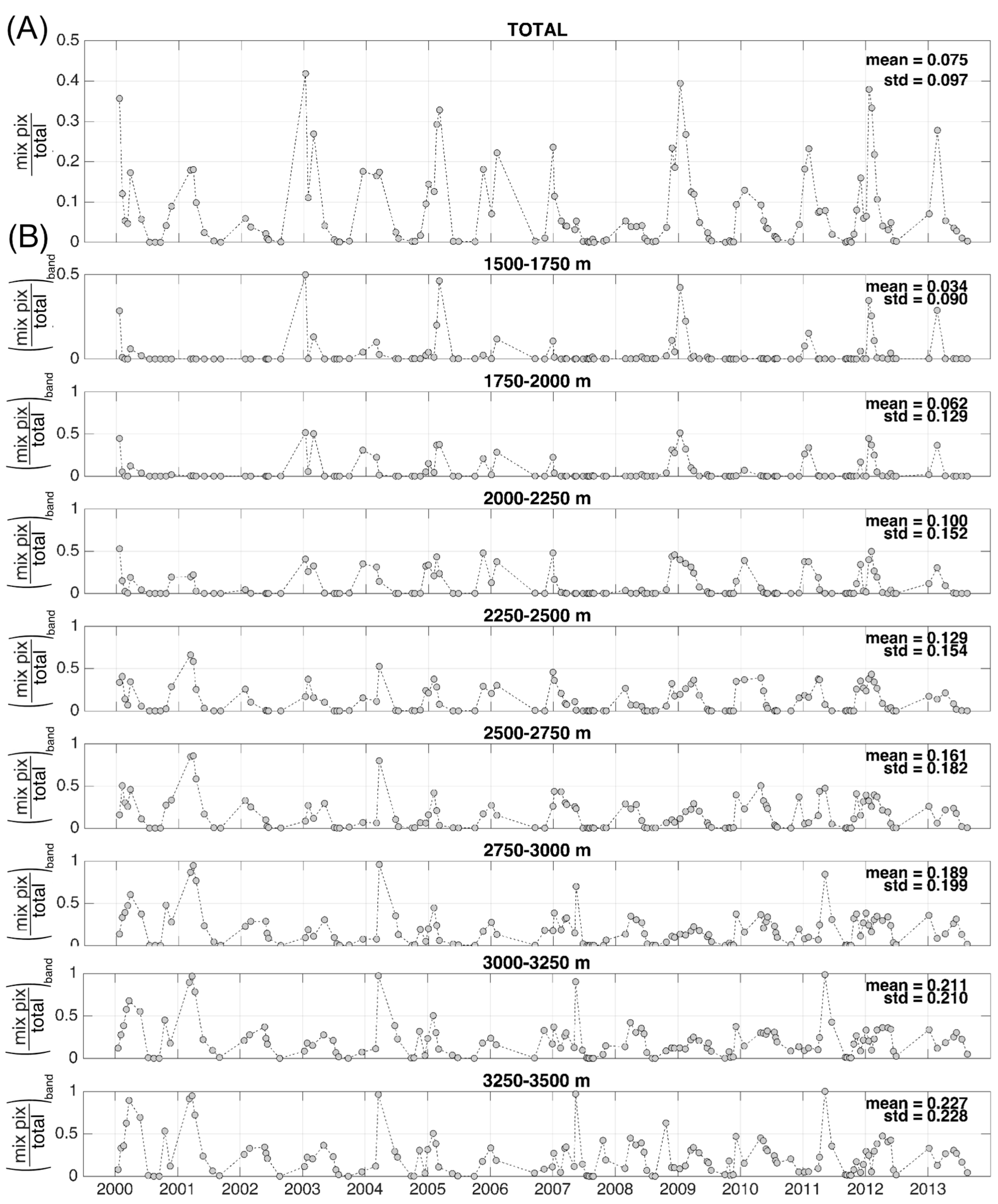
Additionally, the importance of the mixed pixels can be assessed from the fractional maps. Figure 9 shows the fraction of mixed pixels in the study area during the 2000–2013 period, both globally and distributed within altitudinal bands. Mixed pixels can reach up to 40% of the area (Figure 9A) during wet and cold years, being the annual maximum values usually found at the early stages of the melting phases. As expected, the fraction of mixed pixels increases with the altitude, being frequently found in the highest areas, where complete cover is reached every year and persistence can be longer, the snowpack evolving following patchy but persistent patterns well into the spring and even the summer season. On the contrary, in the low altitude bands, where few snowfalls take place and the snow cover may quickly disappear, the mixed pixels are only significant for the extreme events that can take place in certain years. Over 2750 m a.s.l., mixed pixels might reach the 100% of the area during some spring days.
5. Discussion
The results show the importance of patchy areas in semiarid regions such as the study site, and their persistence during the late spring and early summer during specific years; the use of Landsat imagery is key to accurately assess the snow regime in these regions during the periods where the snow cover is not complete. The availability of TP images provided efficient information to estimate the uncertainty of each algorithm and assess their adequacy to approximate the snow cover area in these sites.
Moreover, the results provide some basis to identify criteria on which to make decisions regarding the adoption of each kind of approach. The SMA provided generally better results than the binary approach, since the latter generally overestimated the presence of snow. However, from Table 2 it can be noted that the error associated with each method is quite similar (a maximum value of 11.1% and 9.9% for the binary and fractional approaches, respectively) when the snow presence is important, and the SCA is higher than the 85% of the study area. Below a 33% threshold, the performance of both methods is less accurate, those from the binary approach offering the most limited results due to large overestimation. In the intermediate range, the SMA proves to be the best approach. Additionally, both methods showed 1% of the study area as the detection limit for snow cover area. Despite these thresholds having been obtained over a limited number of images and further work being needed to validate such ranges and thresholds, they represent a varied set of dates and stages during the snow season, and they show the usefulness of combining TP and satellite data to assess the snow cover evolution in semiarid regions. Another important aspect to mention related to uncertainty is the spatial resolution of the remote sensing source; the selection of a greater cell size, as for example MODIS [28], in Painter et al. (2009), could reduce the global errors. Nevertheless, due to the size scale of the snow patches characteristic of snow distribution over these regions, the use of Landsat or any other high-resolution sources is required.
The use of SMA also allows for the spatial assessment of areas where snowfalls can be significant and/or frequent but persistence is not enhanced by the local conditions. The results indicate the areas in which patchy conditions prevail; the availability of SCF maps with a reasonably high spatial resolution is key for the calibration and validation of snow models, and hydrological models, and further assessment of water resources. The seasonal analysis distributed over altitude bands is particularly relevant to identify the more vulnerable areas facing potential changes of the snow regime due to global warming and climate variability, and trace such changes. The future shifts of the occurrence and prevailing of snow patches (i.e., mixed pixels in the images) in these regions can be a powerful indicator for an early detection of changes in the snow regime and its associated services in mountainous regions.
6. Conclusions
In this work, the distribution of the snow cover under highly variable conditions was obtained using Landsat imagery. Two methodologies, binary and fractional approaches, were tested against high-resolution snow cover maps obtained from terrestrial pictures. SCF maps estimated by SMA proved to be a powerful tool for providing time map series, even using spectral signatures from general libraries, showing an improvement larger as the snow cover becomes more discontinuous. The SMA allowed for an adequate estimation of the coverage of snow on a 30-m pixel basis, which avoids large overestimations that may result from a simple binary covered/non-covered classification analysis during melting periods. This is especially important in these semiarid mountainous regions where the particular snow dynamics favors the appearance of patchy areas.
The importance of mixed pixels was satisfactorily quantified from the results of SMA distributed within altitudinal bands in the study area, being their occurrence more representative as altitude increases. A threshold altitude of 2750 m a.s.l. over which mixed pixels may reach the total area of the altitudinal band was identified; this highlights the importance of applying fractional methods to trace the snowpack evolution in these semiarid regions, and its spatial patterns.
The combination of terrestrial and satellite imagery allows for a cost-effective method to obtain snow map series with adequate accuracy. Not only the uncertainty assessment but also the variety of stages identified in the TP led to a first estimation to discriminate operational domains for algorithm selection. Both binary and SMA methods provided satisfactory results when the snow cover was above 85% of the study area; below this threshold, the use of SMA is clearly recommended. This is particularly relevant when the SCF maps are used to calibrate and validate snow and hydrological models, since the propagation of errors from the binary approach might result in too large overestimation of the snow amount and distribution.
Acknowledgments
This work was funded by the Spanish Ministry of Economy and Competitiveness—MINECO (Research Project CGL2014-58508R, “Global monitoring system for snow areas in Mediterranean regions: trends analysis and implications for water resource management in Sierra Nevada”). Moreover, this research was partially developed within the framework of the Panta Rhei Research Initiative of the International Association of Hydrological Science (IAHS) in the Working Group on Water and Energy Fluxes in a Changing Environment.
Author Contributions
R.P. was responsible of analyzing and processing the data and communicating with the journal. J.H. contributed in technical details, terrestrial photography acquisition and treatment of remote sensing information and M.J.P. was responsible for overseeing the research and providing critical insight and recommendations regarding the focus, structure and content of the paper. All authors participated in the writing and proofreading throughout the publication process.
Conflicts of Interest
The authors declare no conflict of interest.
References
- Barnett, T.P.; Adam, J.C.; Lettenmaier, D.P. Potential impacts of a warming climate on water availability in snow-dominated regions. Nature 2005, 438, 303–309. [Google Scholar] [CrossRef] [PubMed]
- Giorgi, F. Climate change hot-spots. Geophys. Res. Lett. 2006, 33, L08707. [Google Scholar] [CrossRef]
- Aguilar, C.; Herrero, J.; Polo, M.J. Topographic effects on solar radiation distribution in mountainous watersheds and their influence on reference evapotranspiration estimates at watershed scale. Hydrol. Earth Syst. Sci. 2010, 14, 2479–2494. [Google Scholar] [CrossRef] [Green Version]
- López-Moreno, J.I.; Vicente-Serrano, S.M.; Morán-Tejeda, E.; Lorenzo-Lacruz, J.; Kenawy, A.; Beniston, M. Effects of the North Atlantic Oscillation (NAO) on combined temperature and precipitation winter modes in the Mediterranean mountains: Observed relationships and projections for the 21st century. Glob. Planet. Chang. 2011, 77, 62–76. [Google Scholar] [CrossRef]
- Kuentz, A.; Arheimer, B.; Hundecha, Y.; Wagener, T. Understanding hydrologic variability across Europe through catchment classification. Hydrol. Earth Syst. Sci. 2017, 21, 2863–2879. [Google Scholar] [CrossRef]
- Ionita, M.; Tallaksen, L.M.; Kingston, D.G.; Stagge, J.H.; Laaha, G.; Van Lanen, H.A.J.; Scholz, P.; Chelcea, S.M.; Haslinger, K. The European 2015 drought from a climatological perspective. Hydrol. Earth Syst. Sci. 2017, 21, 1397–1419. [Google Scholar] [CrossRef]
- Garambois, P.A.; Roux, H.; Larnier, K.; Castaings, W.; Dartus, D. Characterization of process-oriented hydrologic model behavior with temporal sensitivity analysis for flash floods in Mediterranean catchments. Hydrol. Earth Syst. Sci. 2013, 17, 2305–2322. [Google Scholar] [CrossRef] [Green Version]
- Pimentel, R.; Herrero, J.; Polo, M.J. Subgrid parameterization of snow distribution at a Mediterranean site using terrestrial photography. Hydrol. Earth Syst. Sci. 2017, 21, 805–820. [Google Scholar] [CrossRef]
- Pimentel, R.; Herrero, J.; Zeng, Y.; Su, Z.; Polo, M.J. Study of Snow Dynamics at Subgrid Scale in Semiarid Environments Combining Terrestrial Photography and Data Assimilation Techniques. J. Hydrometeorol. 2015, 16, 563–578. [Google Scholar] [CrossRef]
- Ménard, C.B.; Essery, R.; Pomeroy, J. Modelled sensitivity of the snow regime to topography, shrub fraction and shrub height. Hydrol. Earth Syst. Sci. 2014, 18, 2375–2392. [Google Scholar] [CrossRef] [Green Version]
- Winstral, A.; Elder, K.; Davis, R.E. Spatial Snow Modeling of Wind-Redistributed Snow Using Terrain-Based Parameters. J. Hydrometeorol. 2002, 3, 524–538. [Google Scholar] [CrossRef]
- Pimentel, R.; Aguilar, C.; Herrero, J.; Pérez-Palazón, M.J.; Polo, M.J. Comparison between Snow Albedo Obtained from Landsat TM, ETM+ Imagery and the SPOT VEGETATION Albedo Product in a Mediterranean Mountainous Site. Hydrology 2016, 3, 10. [Google Scholar] [CrossRef]
- Notarnicola, C.; Duguay, M.; Moelg, N.; Schellenberger, T.; Tetzlaff, A.; Monsorno, R.; Costa, A.; Steurer, C.; Zebisch, M. Snow Cover Maps from MODIS Images at 250 m Resolution, Part 1: Algorithm Description. Remote Sens. 2013, 5, 110–126. [Google Scholar] [CrossRef]
- Notarnicola, C.; Duguay, M.; Moelg, N.; Schellenberger, T.; Tetzlaff, A.; Monsorno, R.; Costa, A.; Steurer, C.; Zebisch, M. Snow Cover Maps from MODIS Images at 250 m Resolution, Part 2: Validation. Remote Sens. 2013, 5, 1568–1587. [Google Scholar] [CrossRef]
- Dozier, J.; Painter, T.H. Multispectral and Hyperspectral Remote Sensing of Alpine Snow Properties. Annu. Rev. Earth Planet. Sci. 2004, 32, 465–494. [Google Scholar] [CrossRef]
- Cui, Y.; Xiong, C.; Lemmetyinen, J.; Shi, J.; Jiang, L.; Peng, B.; Li, H.; Zhao, T.; Ji, D.; Hu, T. Estimating Snow Water Equivalent with Backscattering at X and Ku Band Based on Absorption Loss. Remote Sens. 2016, 8, 505. [Google Scholar] [CrossRef]
- Gao, Y.; Xie, H.; Lu, N.; Yao, T.; Liang, T. Toward advanced daily cloud-free snow cover and snow water equivalent products from Terra–Aqua MODIS and Aqua AMSR-E measurements. J. Hydrol. 2010, 385, 23–35. [Google Scholar] [CrossRef]
- Thirel, G.; Notarnicola, C.; Kalas, M.; Zebisch, M.; Schellenberger, T.; Tetzlaff, A.; Duguay, M.; Mölg, N.; Burek, P.; de Roo, A. Assessing the quality of a real-time Snow Cover Area product for hydrological applications. Remote Sens. Environ. 2012, 127, 271–287. [Google Scholar] [CrossRef]
- Parajka, J.; Blöschl, G. The value of MODIS snow cover data in validating and calibrating conceptual hydrologic models. J. Hydrol. 2008, 358, 240–258. [Google Scholar] [CrossRef]
- Sade, R.; Rimmer, A.; Litaor, M.I.; Shamir, E.; Furman, A. Snow surface energy and mass balance in a warm temperate climate mountain. J. Hydrol. 2014, 519, 848–862. [Google Scholar] [CrossRef]
- Rosenthal, W.; Dozier, J. Automated Mapping of Montane Snow Cover at Subpixel Resolution from the Landsat Thematic Mapper. Water Resour. Res. 1996, 32, 115–130. [Google Scholar] [CrossRef]
- Selkowitz, D.J.; Forster, R.R. Automated mapping of persistent ice and snow cover across the western U.S. with Landsat. ISPRS J. Photogramm. Remote Sens. 2016, 117, 126–140. [Google Scholar] [CrossRef]
- Crawford, C.J.; Manson, S.M.; Bauer, M.E.; Hall, D.K. Multitemporal snow cover mapping in mountainous terrain for Landsat climate data record development. Remote Sens. Environ. 2013, 135, 224–233. [Google Scholar] [CrossRef]
- Pimentel, R.; Herrero, J.; Polo, M.J. Terrestrial photography as an alternative to satellite images to study snow cover evolution at hillslope scale. Proc. SPIE 2012. [Google Scholar] [CrossRef]
- Silasari, R.; Parajka, J.; Ressl, C.; Strauss, P.; Blöschl, G. Potential of time-lapse photography for identifying saturation area dynamics on agricultural hillslopes. Hydrol. Process. 2017, 31, 3610–3627. [Google Scholar] [CrossRef]
- Corripio, J.G. Snow surface albedo estimation using terrestrial photography. Int. J. Remote Sens. 2004, 25, 5705–5729. [Google Scholar] [CrossRef]
- Hall, D.K.; Riggs, G.A.; Salomonson, V.V.; DiGirolamo, N.E.; Bayr, K.J. MODIS snow-cover products. Remote Sens. Environ. 2002, 83, 181–194. [Google Scholar] [CrossRef]
- Painter, T.H.; Rittger, K.; McKenzie, C.; Slaughter, P.; Davis, R.E.; Dozier, J. Retrieval of subpixel snow covered area, grain size, and albedo from MODIS. Remote Sens. Environ. 2009, 113, 868–879. [Google Scholar] [CrossRef]
- Anderson, R.S.; Jiménez-Moreno, G.; Carrión, J.S.; Pérez-Martínez, C. Postglacial history of alpine vegetation, fire, and climate from Laguna de Río Seco, Sierra Nevada, southern Spain. Quat. Sci. Rev. 2011, 30, 1615–1629. [Google Scholar] [CrossRef]
- Heywood, V.H. The Mediterranean flora in the context of world biodiversity. Ecol. Mediterr. 1995, 21, 11–18. [Google Scholar]
- Pérez-Palazón, M.J.; Pimentel, R.; Herrero, J.; Aguilar, C.; Perales, J.M.; Polo, M.J. Extreme values of snow-related variables in Mediterranean regions: Trends and long-term forecasting in Sierra Nevada (Spain). In Proceedings of the International Association of Hydrological Sciences; Copernicus GmbH: Gottingen, Germany, 2015; Volume 369, pp. 157–162. [Google Scholar]
- Dumont, M.; Brissaud, O.; Picard, G.; Schmitt, B.; Gallet, J.-C.; Arnaud, Y. High-accuracy measurements of snow Bidirectional Reflectance Distribution Function at visible and NIR wavelengths—Comparison with modeling results. Atmos. Chem. Phys. 2010, 10, 2507–2520. [Google Scholar] [CrossRef] [Green Version]
- Liang, S.; Fang, H.; Chen, M. Atmospheric correction of Landsat ETM+ land surface imagery. I. Methods. IEEE Trans. Geosci. Remote Sens. 2001, 39, 2490–2498. [Google Scholar] [CrossRef]
- Liang, S.; Stroeve, J.C.; Grant, I.F.; Strahler, A.H.; Duvel, J.P. Angular corrections to satellite data for estimating earth radiation budget. Remote Sens. Rev. 2000, 18, 103–136. [Google Scholar] [CrossRef]
- Chander, G.; Markham, B.L.; Helder, D.L. Summary of current radiometric calibration coefficients for Landsat MSS, TM, ETM+, and EO-1 ALI sensors. Remote Sens. Environ. 2009, 113, 11. [Google Scholar] [CrossRef]
- Moran, M.S.; Jackson, R.D.; Slater, P.N.; Teillet, P.M. Evaluation of simplified procedures for retrieval of land surface reflectance factors from satellite sensor output. Remote Sens. Environ. 1992, 41, 169–184. [Google Scholar] [CrossRef]
- Chavez, P.S., Jr. Image Based Atmospheric Corrections-Revisited and Improved. Photogramm. Eng. Remote Sens. 1996, 62, 1025–1036. [Google Scholar]
- Chavez, P.S. An improved dark-object subtraction technique for atmospheric scattering correction of multispectral data. Remote Sens. Environ. 1988, 24, 459–479. [Google Scholar] [CrossRef]
- Hagolle, O.; Huc, M.; Villa Pascual, D.; Dedieu, G. A Multi-Temporal and Multi-Spectral Method to Estimate Aerosol Optical Thickness over Land, for the Atmospheric Correction of FormoSat-2, LandSat, VENμS and Sentinel-2 Images. Remote Sens. 2015, 7, 2668–2691. [Google Scholar] [CrossRef]
- Gilabert, M.A.; Conese, C.; Maselli, F. An atmospheric correction method for the automatic retrieval of surface reflectances from TM images. Int. J. Remote Sens. 1994, 15, 2065–2086. [Google Scholar] [CrossRef]
- Song, C.; Woodcock, C.E.; Seto, K.C.; Lenney, M.P.; Macomber, S.A. Classification and Change Detection Using Landsat TM Data. Remote Sens. Environ. 2001, 75, 230–244. [Google Scholar] [CrossRef]
- Karnieli, A.; Ben-Dor, E.; Bayarjargal, Y.; Lugasi, R. Radiometric saturation of Landsat-7 ETM+ data over the Negev Desert (Israel): Problems and solutions. Int. J. Appl. Earth Obs. Geoinf. 2004, 5, 219–237. [Google Scholar] [CrossRef]
- Tucker, C.J. Red and photographic infrared linear combinations for monitoring vegetation. Remote Sens. Environ. 1979, 8, 127–150. [Google Scholar] [CrossRef]
- Hantson, S.; Chuvieco, E. Evaluation of different topographic correction methods for Landsat imagery. Int. J. Appl. Earth Obs. Geoinf. 2011, 13, 691–700. [Google Scholar] [CrossRef]
- Dozier, J. Spectral signature of alpine snow cover from the landsat thematic mapper. Remote Sens. Environ. 1989, 28, 9–22. [Google Scholar] [CrossRef]
- Herrero, J.; Polo, M.J.; Losada, M.A. Snow evolution in Sierra Nevada (Spain) from an energy balance model validated with Landsat TM data. Proc. SPIE 2011. [Google Scholar] [CrossRef]
- Roberts, D.A.; Gardner, M.; Church, R.; Ustin, S.; Scheer, G.; Green, R.O. Mapping chaparral in the Santa Monica Mountains using multiple endmember spectral mixture models. Remote Sens. Environ. 1998, 65, 267–276. [Google Scholar] [CrossRef]
- Fiume, E.L. The Mathematical Structure of Raster Graphics; Academic Press: New York, NY, USA, 2014; ISBN 978-1-4832-6082-2. [Google Scholar]
- Foley, J.D. Computer Graphics: Principles and Practice; Addison-Wesley Professional: Reading, MA, USA, 1996; ISBN 978-0-201-84840-3. [Google Scholar]
Figure 1.
(A) Location of Sierra Nevada Mountain in Spain; (B) Sierra Nevada Mountain range, limits of the Natural and National Parks (dark and light blue respectively) and 1500 m a.s.l. elevation line (black line); (C) Location of the control area monitored by terrestrial photography at Durcal hillside.
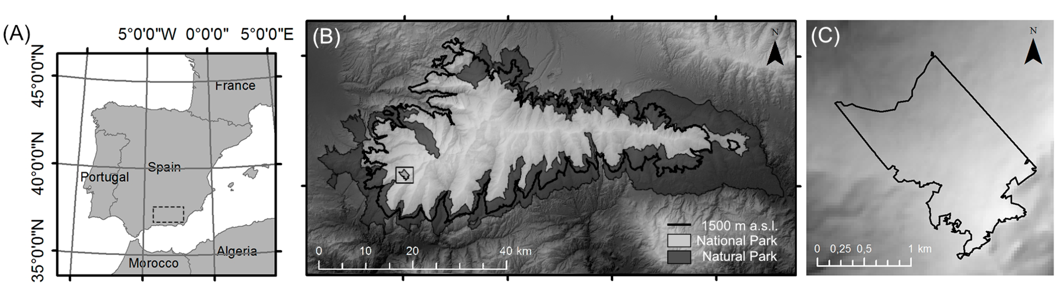
Figure 2.
Landsat scenes, TM (grey dots) and ETM+ (black crosses) analyzed throughout the study period 2000–2013 over Sierra Nevada Mountain. Available Terrestrial Photography (TP) used as validation dataset (red dots) over the control area throughout the validation period (2009–2013).
Figure 2.
Landsat scenes, TM (grey dots) and ETM+ (black crosses) analyzed throughout the study period 2000–2013 over Sierra Nevada Mountain. Available Terrestrial Photography (TP) used as validation dataset (red dots) over the control area throughout the validation period (2009–2013).

Figure 3.
(A) Evolution of the averaged snow cover fraction in Sierra Nevada Mountain above the threshold altitude of 1000 m throughout the study period (2000–2013) from both binary (grey dots) and fractional (black crosses) algorithms, and (B) the associated standard deviation values, together with their difference.
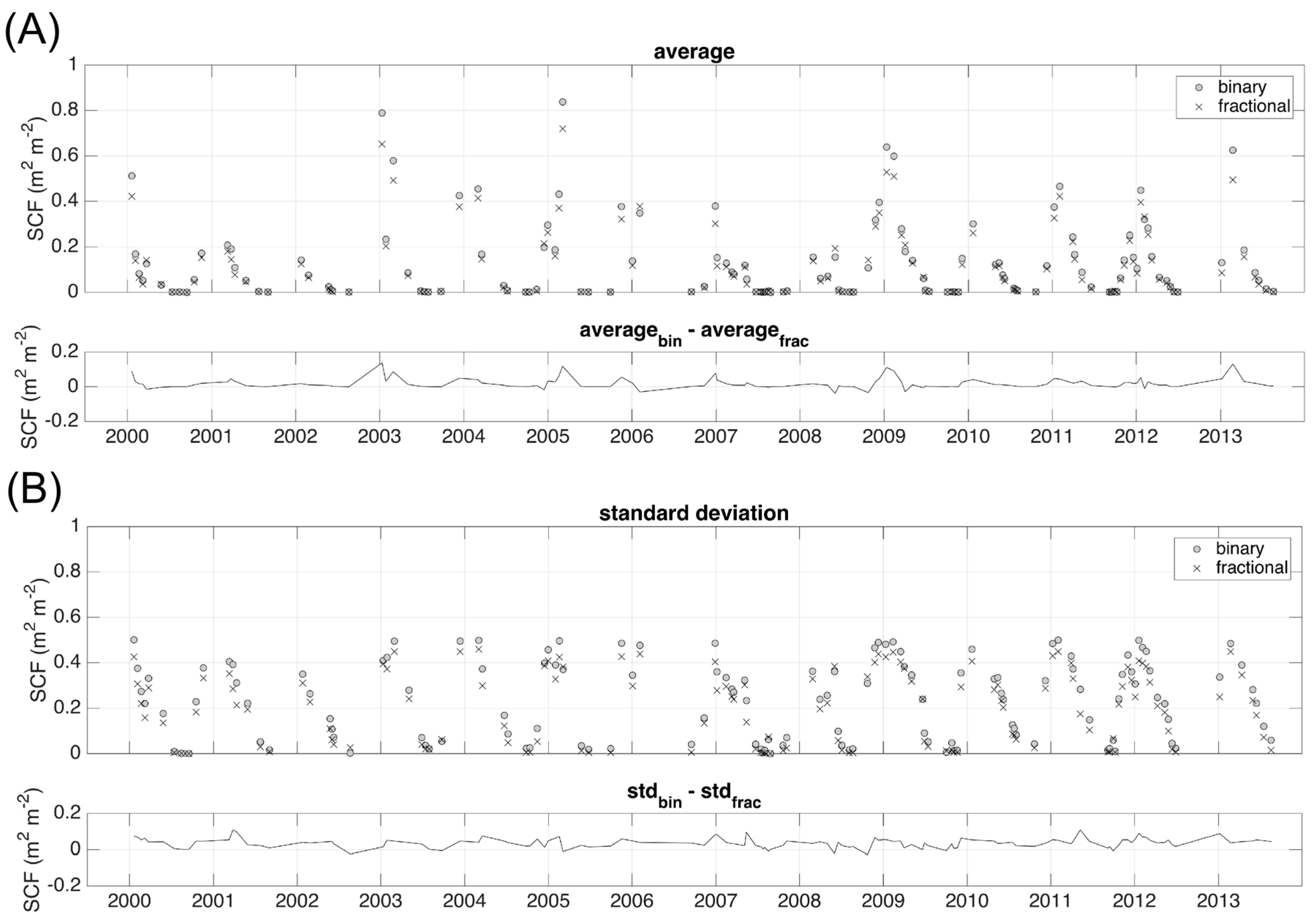
Figure 4.
Distribution of the mean and standard deviation of the SCF (m2 m−2) over the study area during the study period 2000–2013 using a binary and a fractional algorithm.
Figure 4.
Distribution of the mean and standard deviation of the SCF (m2 m−2) over the study area during the study period 2000–2013 using a binary and a fractional algorithm.

Figure 5.
(A) Selected examples of different stages during the snow season: accumulation—complete cover (10 January 2011), beginning of the spring melting (16 June 2013) and end of the melting (29 June 2009), using the Landsat (binary and fractional) methodologies and TP at the control area. (B) Evolution of the three metrics (precision, recall and accuracy) used during the validation period (2009–2013) for both methodologies (right); distribution function (boxplot, the central line and the upper and lower edges of the box represent the median, 75th and 25th percentiles respectively; the black whiskers extend to the extreme values considered in the analysis; and the red crosses are the outliers) of each metric for each method (left).
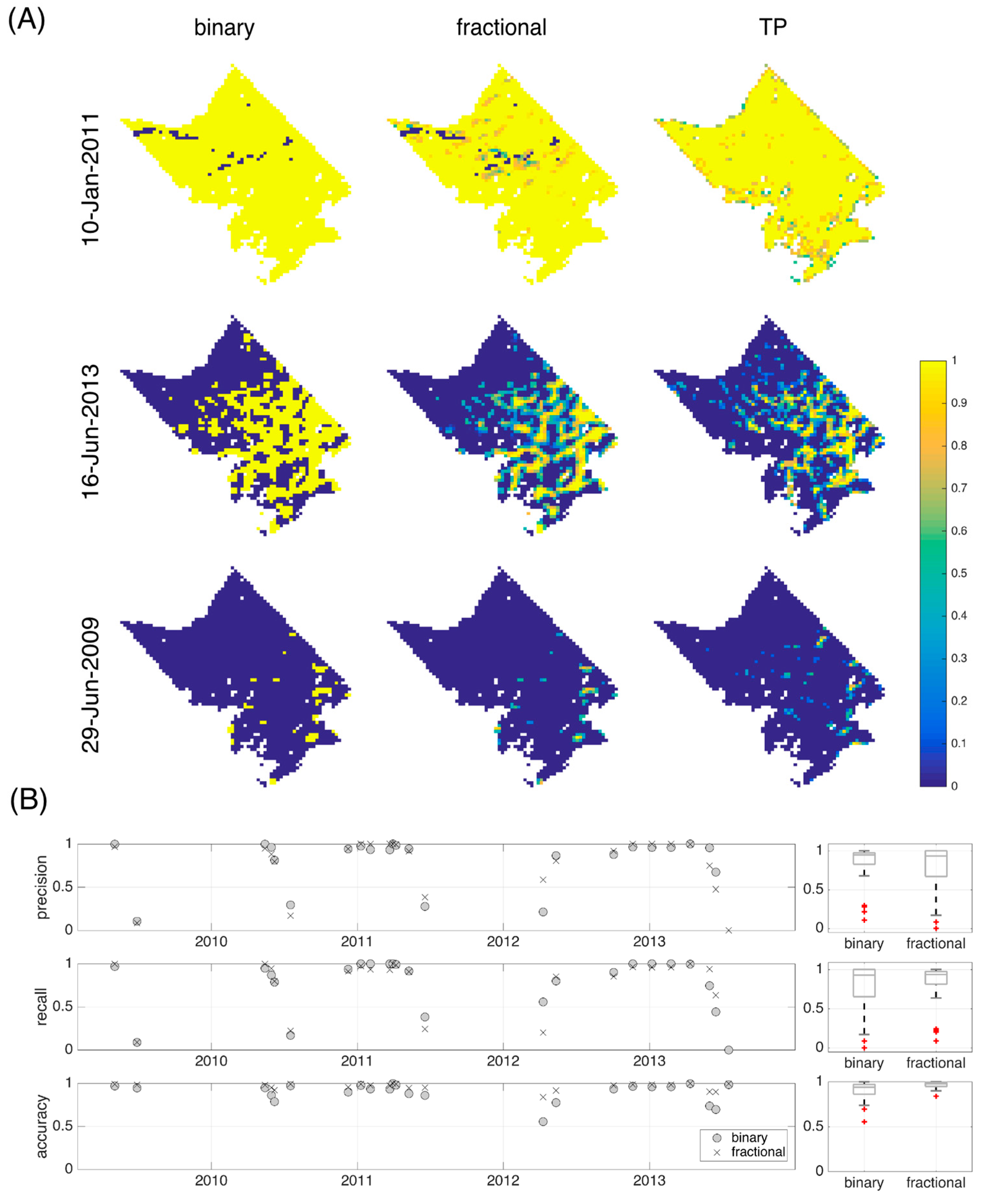
Figure 6.
Evolution of SCF over the control area throughout the validation period (2009–2013) (right). Dispersion graph comparing the evaluated SCF obtained from Landsat with the validation dataset obtained calculated using TP (left).
Figure 6.
Evolution of SCF over the control area throughout the validation period (2009–2013) (right). Dispersion graph comparing the evaluated SCF obtained from Landsat with the validation dataset obtained calculated using TP (left).

Figure 7.
Left: Temporal evolution of the average SCF value at the Sierra Nevada range during the study period for the whole study area (A) and distributed within 250 m-range elevation bands (B). Right: Monthly distribution of the average SCF values (black dots) and monthly mean value (red line) for each case.

Figure 8.
(A) Cumulative distribution function (cdf) of the average SCF in the study area for the 2000–2013 period. (B) Spatial distribution of selected percentiles (5th, 10th, 25th, 50th, 75th, 90th and 95th) of the pixel-SCF cdfs.
Figure 8.
(A) Cumulative distribution function (cdf) of the average SCF in the study area for the 2000–2013 period. (B) Spatial distribution of selected percentiles (5th, 10th, 25th, 50th, 75th, 90th and 95th) of the pixel-SCF cdfs.

Figure 9.
(A) Temporal evolution of the fraction of mixed pixels at the Sierra Nevada range during the study period for the whole study area (number of mixed pixels/total pixels) and (B) distributed within 250 m-range elevation bands (number of mixed pixels/pixels in the elevation band).
Figure 9.
(A) Temporal evolution of the fraction of mixed pixels at the Sierra Nevada range during the study period for the whole study area (number of mixed pixels/total pixels) and (B) distributed within 250 m-range elevation bands (number of mixed pixels/pixels in the elevation band).


Table 1.
Mean and standard deviation, in brackets, of the main meteorological variables in Sierra Nevada Mountains from 2009 to 2013, calculated over both south and north faces and for low areas (below 2000 m a.s.l.) and high areas (above 2000 m a.s.l.).
Table 1.
Mean and standard deviation, in brackets, of the main meteorological variables in Sierra Nevada Mountains from 2009 to 2013, calculated over both south and north faces and for low areas (below 2000 m a.s.l.) and high areas (above 2000 m a.s.l.).
| Facing | Elevation | Precipitation | Temperature | Radiation | Wind Speed |
|---|---|---|---|---|---|
| (mm) | (°C) | (MJ m‒2 day‒1) | (ms‒1) | ||
| South face | High areas | 783.3 (35.8) | 7.8 (6.9) | 11.1 (1.1) | 8.2 (0.5) |
| Low areas | 503.7 (14.8) | 14.8 (7.4) | 9.5 (1.5) | 3.2 (1.4) | |
| North face | High areas | - | 6.8 (5.6) | 10.9 (0.3) | 5.1 (2.2) |
| Low areas | 526.7 (116.3) | 9.7 (4.5) | 9.4 (1.2) | 2.4 (1.3) |
Table 2.
Snow cover area calculated from Landsat-binary (ABIN), Landsat-fractional (AFRAC) and TP (ATP), and absolute and relative error associated to each Landsat map and date at the 2-km2 validation control area.
Table 2.
Snow cover area calculated from Landsat-binary (ABIN), Landsat-fractional (AFRAC) and TP (ATP), and absolute and relative error associated to each Landsat map and date at the 2-km2 validation control area.
| Date | (km2) | (km2) | (km2) | (km2) | (km2) | ||
|---|---|---|---|---|---|---|---|
| 4 May 2009 | 1.90 | 1.88 | 1.71 | 0.19 | 0.111 | 0.17 | 0.099 |
| 29 June 2009 | 0.06 | 0.04 | 0.04 | 0.02 | 0.500 | 0.00 | 0.000 |
| 15 May 2010 | 1.90 | 1.88 | 1.67 | 0.23 | 0.138 | 0.21 | 0.126 |
| 31 May 2010 | 1.58 | 1.35 | 1.24 | 0.34 | 0.274 | 0.11 | 0.089 |
| 8 June 2010 | 1.03 | 0.80 | 0.82 | 0.21 | 0.256 | −0.02 | −0.024 |
| 18 July 2010 | 0.04 | 0.02 | 0.02 | 0.02 | 1.000 | 0.00 | 0.000 |
| 9 December 2010 | 1.64 | 1.33 | 1.45 | 0.19 | 0.131 | −0.12 | −0.083 |
| 10 January 2011 | 1.86 | 1.83 | 1.83 | 0.03 | 0.016 | 0.00 | 0.000 |
| 3 February 2011 | 1.79 | 1.75 | 1.83 | −0.04 | −0.022 | −0.08 | −0.044 |
| 31 March 2011 | 1.90 | 1.90 | 1.83 | 0.07 | 0.038 | 0.07 | 0.038 |
| 8 April 2011 | 1.88 | 1.81 | 1.81 | 0.07 | 0.039 | 0.00 | 0.000 |
| 10 May 2011 | 1.67 | 1.03 | 1.45 | 0.22 | 0.152 | −0.42 | −0.290 |
| 19 June 2011 | 0.17 | 0.10 | 0.17 | 0.00 | 0.000 | −0.07 | −0.412 |
| 12 May 2012 | 1.31 | 1.01 | 0.91 | 0.40 | 0.440 | 0.10 | 0.110 |
| 7 January 2013 | 1.83 | 1.69 | 1.83 | 0.00 | 0.000 | −0.14 | −0.077 |
| 24 February 2013 | 1.83 | 1.81 | 1.83 | 0.00 | 0.000 | −0.02 | −0.011 |
| 13 April 2013 | 1.90 | 1.88 | 1.83 | 0.07 | 0.038 | 0.05 | 0.027 |
| 31 May 2013 | 1.73 | 1.46 | 1.08 | 0.65 | 0.602 | 0.38 | 0.352 |
| 16 June 2013 | 0.74 | 0.46 | 0.36 | 0.38 | 1.056 | 0.10 | 0.278 |
| 18 July 2013 | 0.02 | 0.02 | 0.00 | 0.02 | 0.02 |
© 2017 by the authors. Licensee MDPI, Basel, Switzerland. This article is an open access article distributed under the terms and conditions of the Creative Commons Attribution (CC BY) license (http://creativecommons.org/licenses/by/4.0/).
Share and Cite
MDPI and ACS Style
Pimentel, R.; Herrero, J.; Polo, M.J. Quantifying Snow Cover Distribution in Semiarid Regions Combining Satellite and Terrestrial Imagery. Remote Sens. 2017, 9, 995. https://doi.org/10.3390/rs9100995
AMA Style
Pimentel R, Herrero J, Polo MJ. Quantifying Snow Cover Distribution in Semiarid Regions Combining Satellite and Terrestrial Imagery. Remote Sensing. 2017; 9(10):995. https://doi.org/10.3390/rs9100995
Chicago/Turabian StylePimentel, Rafael, Javier Herrero, and María José Polo. 2017. "Quantifying Snow Cover Distribution in Semiarid Regions Combining Satellite and Terrestrial Imagery" Remote Sensing 9, no. 10: 995. https://doi.org/10.3390/rs9100995
Note that from the first issue of 2016, this journal uses article numbers instead of page numbers. See further details here.