Detecting Forest Disturbance in Northeast China from GLASS LAI Time Series Data Using a Dynamic Model


1
State Key Laboratory of Remote Sensing Science, Jointly Sponsored by Beijing Normal University and Institute of Remote Sensing and Digital Earth of Chinese Academy of Sciences, Beijing 100875, China
2
Beijing Engineering Research Center for Global Land Remote Sensing Products, Institute of Remote Sensing Science and Engineering, Faculty of Geographical Science, Beijing Normal University, Beijing 100875, China
*
Author to whom correspondence should be addressed.
Remote Sens. 2017, 9(12), 1293; https://doi.org/10.3390/rs9121293
Submission received: 27 October 2017
/
Revised: 23 November 2017
/
Accepted: 9 December 2017
/
Published: 12 December 2017
(This article belongs to the Special Issue Advances in Quantitative Remote Sensing in China – In Memory of Prof. Xiaowen Li)
Abstract
:Large-scale forest disturbance often leads to changes in forest cover and structure, which imposes a great uncertainty in the estimation of the forest carbon cycle and biomass and affects other applications. In northeastern China, the Daxinganling region has abundant forest resources, where the forest coverage is about 30%. The Global LAnd Surface Satellite (GLASS) leaf area index (LAI) time series data provide important information to monitor the possible change of forests. In this study, we developed a new method to detect forest disturbances using GLASS LAI data over the Daxinganling region of Northeast China. As a dynamic model, the season-trend model has a higher sensitivity toward a seasonal change in LAI. Based on the accumulation of multi-year GLASS LAI products from 1997 to 2002, the dynamic model of LAI time series for each pixel is established first. The time-stepping modeling (TSM) process was designed by using the season-trend method, and sequential tests for detecting disturbances from a time series of pixels. Significant changes in the model parameters were captured as disturbance signals. Then, the near-infrared and shortwave-infrared bands of Moderate Resolution Imaging Spectroradiometer (MODIS) surface reflectance are used as auxiliary information to distinguish the types of forest disturbances. Here, the algorithm led to the detection of two different types of disturbances: fire and other (e.g., insect, drought, deforestation). In this study, we took the forest region as the study area, used the 8-day composite GLASS LAI data at 1000-m spatial resolution to identify each pixel as a fire disturbance, other disturbance, or non-disturbance. Validation was performed using reference burned area data derived from Landsat 30 m imagery. Results were also compared with the MCD64 product. The validation results were based on confusion matrices showing the overall accuracy (OA) exceeded 92% for our method and the MCD64 product. Statistical tests identified that TSM’s product accuracy is higher than that of MCD64. This study demonstrated that the TSM algorithm using a season-trend model provides a simple and automated approach to identify and map forest disturbance.
1. Introduction
Forest disturbances are discrete events that cause tree mortality and destruction of plant biomass. An effective method to detect the temporal and spatial distribution of forest disturbance in a large area is to use remote sensing time series data. In many ecological models, accurate monitoring of forest disturbances has a crucial role in Gross Primary Production (GPP) and Net Primary Production (NPP) estimation accuracy and aerosol and biomass estimation [1,2,3,4,5,6,7,8,9,10]. The mapping of precise forest disturbances in large areas provides basic data for wildlife protection and strong support for large-scale vegetation biophysical and structural change monitoring [11]. Based on the needs of various applications, the use of remote sensing data for detecting forest disturbances in a large area has been carried out widely.
Many efficient methods have been proposed to detect changes from image time series. The methods include detecting forest disturbance and recovery [3,12,13], detecting trend and seasonal changes [14,15,16], and extracting seasonality metrics from satellite time series [17,18]. Current remote sensing approaches in monitoring forest disturbance detection are mainly based on vegetation indices (VI) and other vegetation parameters [19,20,21,22,23,24], such as the normalized difference vegetation index (NDVI) and Fraction of Absorbed Photosynthetically Active Radiation (FAPAR) [11], to determine the disturbance by analyzing the changes in a long time series. VI is a common indicator of vegetation disturbance monitoring. Vegetation is relatively fragile in terrestrial ecosystems, and it is also sensitive to the occurrence of disturbances. It is possible to detect the disturbance events effectively by observing the change of vegetation using remote sensing data. NDVI is the most widely used VI; it can show the growth curve of vegetation over time. It is suitable for medium and long-term vegetation growth monitoring, phenophase monitoring, and crop yield estimation. The hotspot and NDVI differencing synergy (HANDS) [19] algorithm was applied to Canadian forests during the 1995–2000 fire seasons using the annual hotspot masks and differencing of the anniversary date of September NDVI composites. HANDS is designed to produce annual maps of burned forests by combining the active fire detection product with NDVI differencing, a common change detection technique. The HANDS method substantially reduces noise levels by requiring that burned areas identified through NDVI differencing be co-located with hotspots. In 2009, Mildrexler used the Moderate Resolution Imaging Spectroradiometer (MODIS) global disturbance index (MGDI) [25] with satellite data to operationally detect large-scale ecosystem disturbances at 1-km resolution. The MGDI algorithm was designed to contrast annual changes in vegetation density and land surface temperature (LST) following disturbance by enhancing the signal to effectively detect the location and intensity of disturbances.
Disturbances from agents such as fire, insect damage, or strong winds are common throughout the world’s forests. Fire is the dominant driver of forest disturbance at the global scale, and fire is one of the most dominant disturbance agents in Northeast China. Currently, the most widely used burned area products are three MODIS data products and three products developed within the fire disturbance project (fire_cci) [26,27,28,29,30,31]. There is a significant difference between the detection results of different products; through a comparison of a variety of products, statistical tests identified that MCD64 was the most accurate, followed by MCD45 [32]. Biomass density varies through time as a result of disturbances; accurate estimates of biomass emissions focuses on identifying disturbances (whether anthropogenic or natural), but it is difficult to meet the application requirements with most of the forest disturbance products.
In this study, we used The Global LAnd Surface Satellite (GLASS) leaf area index (LAI) time series data to detect forest disturbances in Northeast China. We developed a method for disturbance detection in forest land. Based on the season-trend model [15,16], the GLASS LAI data from 1997 to 2002 was taken as the background dataset to model phenological changes of vegetation in forest land, which represents the annual periodic variation curve of LAI without disturbance. The model parameters were used as the reference parameters for identifying disturbance pixels. Every 8 days, GLASS LAI data acquired after 2002 was iteratively added to the background dataset to model the phenological change step by step. The model parameters could be different in each modeling step and were taken as a signal of whether there was a disturbance. These procedures were iterated until the end of a time series or until a change was detected. We call this algorithm the time-stepping modeling (TSM) process. During the monitoring period, the disturbance was detected by the difference between the criteria parameters and the new parameters which were re-simulated by adding a new LAI. The forest disturbance and the natural growth were distinguished by the disturbance index (DI), which is defined in this paper, and the forest disturbance was automatically identified. Finally, the normalized burn ratio (NBR) was used to reclassify the disturbance of vegetation to determine whether it was a burned area. In order to verify the accuracy of the approach, the types and spatial ranges of forest disturbance were detected in a forest region of Northeast China. The detected result was compared with the burned area of MCD64 and the burned area of Landsat, which were calculated using the differenced NBR (dNBR) method. The results demonstrated the validity of our method through experiments in the Daxinganling Mountains, including the effective detection of disturbances based on the TSM process using a dynamic model, and the discrimination of types of disturbances.
2. Materials
2.1. Study Area
We selected the northeast forest area of China as our study area. The region is characterized by a continental monsoon climate. The forests in the region are horizontally divided into four regions of vegetation: the cool temperate deciduous coniferous forest region, the temperate mixed evergreen coniferous-deciduous broad-leaved forest region, the warm temperate deciduous broad-leaved forest region, and the temperate steppe region. Forests of these types account for about 30% of forest in China. Northeastern China has abundant tree species and a variety of forest types, including evergreen needleleaf forest, deciduous needleleaf forest, deciduous broadleaf forest, and mixed forests. Figure 1 shows the location of the study area and the land classification results of 30 m resolution (Figure 1A) and 1000 m resolution (Figure 1B). In subsequent steps, we use 1000 m land classification results.
2.2. Data Processing
The remote sensed data we used in this study include the GLASS LAI product from 1997 to 2003, the “MOD09A1” 500-m MODIS atmospherically-corrected Level 3 8-day surface reflectance products, and the Level 3 MODIS “MCD64A1” monthly burned area products. The MOD09A1 and MCD64A1 data were reprojected from the MODIS sinusoidal projection into the Albers equal area projection at 1000 m resolution. In order to test the performance of the forest disturbance detection approach, Landsat TM images of 2003 were used to create high resolution burned area maps. The maps were taken as a reference to assess our disturbance detection results at 1 km spatial resolution.
The GLASS LAI product was retrieved from time series MODIS and Advanced very-high-resolution radiometer (AVHRR) surface reflectance data using general regression neural networks (GRNNs), and the inter-comparison of GLASS LAI products and other existing operational global LAI products, including MODIS and CYCLOPES, indicate that the GLASS LAI product is the most spatially complete and temporally continuous [33].
The mean phenological change of the LAI was computed for 5 years (1997–2001) on a pixel-by-pixel basis. The mean LAI reflects the undisturbed plant growth phenology and provides a background to assess a departure from the LAI variability. The vegetation in the northeast forest area was dominated by deciduous forests; therefore, LAI at the beginning and end of the year were at a very low level. In order to improve the simulation of the LAI model accuracy by excluding non-growth period data, the input parameters were taken from the 96th day to the 306th day of each year.
The study focuses on forest land. We used land classification data to mask non-forest areas. Land use classification is the result of supervised classification using Landsat data to derive seven categories: forestland, artificial cover, water, shrubland, wetland, cropland, grassland, as shown in Figure 1A. We resampled the spatial resolution of the classifications from 30 m to 1000 m using a mode resampling method, and the land use was divided into two categories: forest land area and non-forest land. The classifications data was reprojected from the UTM projection into the Albers equal area projection. Land use classification results are shown in Figure 1B. The remote sensing data used in the present paper are in Table 1.
3. Methods
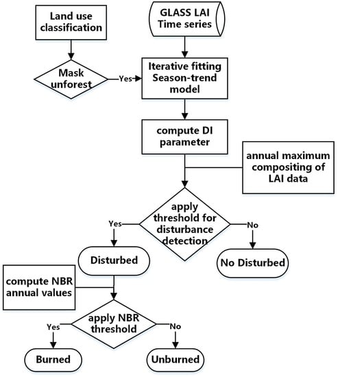
LAI as an indicator of vegetation coverage and vegetation growth status can directly reflect the growth status of vegetation. In the normal growth period of forests, LAI has a similar annual periodic variation. The annual LAI curve also has good continuity, so there is no obvious fluctuations in the curve. When a forest disturbance occurs, such as drought, pest, fire, deforestation, etc., these effects directly affect the LAI, which will be reduced significantly. Through analysis of a long time series of forest LAI data from remote sensing images using our developed dynamic model and the TSM process, we can detect the location and range of the forest disturbances effectively. Figure 2 shows the flow chart of the approach.
3.1. Iterative Algorithm to Detect Forest Disturbance
The season-trend method is a linear regression model proposed by Verbesselt to account for seasonal and trend changes typically occurring within climate-driven biophysical indicators derived from satellite data [15,16]. The model is an additive decomposition model, which is based on the characteristics of the periodic variation of remote sensing data from the vegetation-covered surface. It is assumed that the time series is mainly composed of seasons and trends; thus, the modeling results are obtained using the trends and seasons in the model sequence to be decomposed, as follows
where is the time series observation at time , the intercept , slope , amplitudes , and phases are the unknown simulation parameters, is the number of harmonic terms that should be specified manually, is the frequency of the time series observations, and is the error term at time .
We used three harmonic terms to robustly simulate phenological changes within GLASS LAI time series [34,35]. The formula for LAI time series simulation can be expressed as follows
In a large area of forest disturbance detection, the idea for monitoring techniques is simple. In this paper, the estimation of parameters was performed by iterating through the following steps until reaching the last value of the monitoring period or until a disturbance is detected:
Step 1: Based on a given LAI time series (there are two parts of data: the mean phenological change of 1997–2001 and the year 2002, thus we call it background data), the Equation (2) was used to simulate the LAI time series, the initial simulation parameters (i.e., and in Equation (2)) were used as the reference parameters for detection.
Step 2: The iterative procedure began with a simulation of Y (2003) of Equation (2) by using the season-trend method. The modeling data was a combination of background data and monitoring data. The first LAI data in 2003 was the starting point of the monitoring data for detection, and the parameters of the fitting model were calculated.
Step 3: The size of the window was the same as the background data, the moving width of the window for monitoring data was equal to 1. When we add monitor LAI data to the end of the background data, the first of the background data is removed. The fitting model parameters obtained after adding the monitoring data were compared with the reference parameters to determine whether any change was detected.
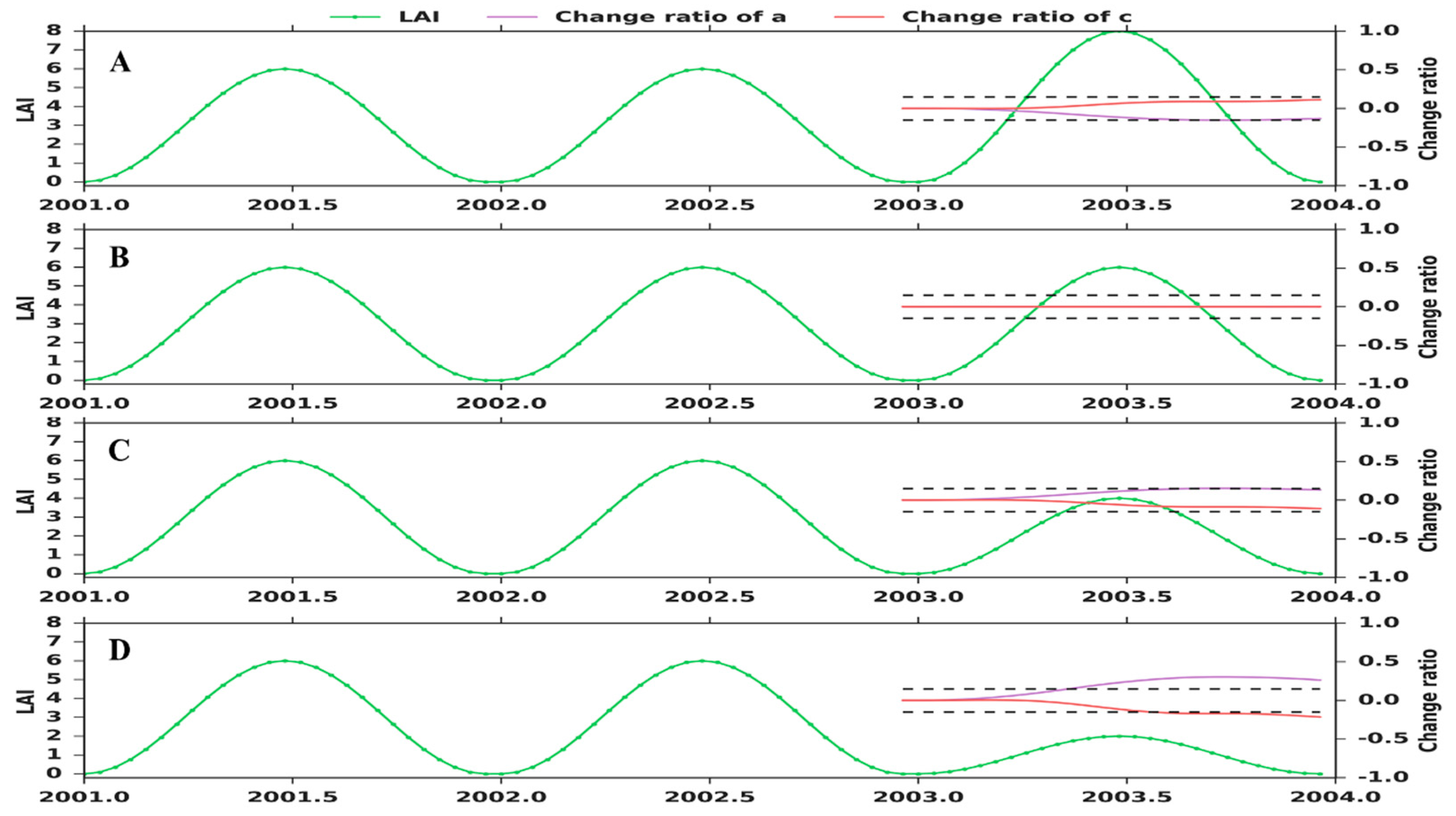
The mean LAI can represent the normal phenological pattern of forests. The LAI of the prior year shows whether forest growth has changed. Through the simulation of background data, the growth structure of the forest can be determined. It can be considered, as the phenology of the previous year occupied a higher weight in the simulation process. These time-stepping modeling processes were iterated until reaching the last value of the monitoring period or until disturbances are detected. Through analysis of the model parameters, the amplitude parameter was found to be the most sensitive to structural changes in the time series, as shown in Figure 3. For the detection of forest disturbances, we defined the and using the following formulas
where () is the value of the parameter c in the initial simulation and () is the value of the parameter c (a) on the n (1 < n < 27) time series used in the monitoring period.
Using a set of simulated LAI data of three years, Figure 3 shows an example of this analysis; four subsets were established within varying degrees of growth. We computed the DI values at each single step length during the disturbance in 2003. Figure 3A illustrates the change in DI in the case of forest growth. With the increase of fitting data, the value of gradually increases, and the value of decreases gradually. Figure 3B illustrates the change in DI value without disturbance. The time series of DI basically did not fluctuate, hovering around zero. Figure 3C illustrates the change in DI value with a certain degree of disturbance. As the disturbance continues, the value of gradually increases, and the value of decreases gradually. Figure 3D illustrates that with the increase in the degree of disturbance, the value of appeared to have a greater degree of reduction, while the value of appeared to increase to a much greater degree. Based on the analysis of the disturbed area, we selected and as our thresholds for detecting those disturbances. In the iterative modeling, when the amplitude of the two parameter changes do not exceed the threshold, forest disturbances will be identified as not occurring. Otherwise, forest disturbances will be detected.
The LAI value of some of the pixels may have been at a low level; therefore, if there is a slight change in LAI it will lead to a disturbance index that appears to have relatively large fluctuations, resulting in the detection of an error. To avoid this problem, we applied annual maximum value compositing to the LAI data. The LAI data were combined into one image representing the maximum LAI detected at every pixel throughout an annual period, and then this was compared with the annual maximum of the previous year’s LAI.
If the LAI maximum of the same pixel had a decrease of 1.5 for two years, it was detected as a disturbance in the previous step. It is possible to be confident that the pixel was disturbed, otherwise, no disturbance had occurred. Any pixels above this threshold were flagged as a disturbance.
3.2. Distinguish the Types of Disturbances
The normalized burn ratio (NBR) [36,37] in form is a modification of the NDVI, except that it uses near-infrared (NIR) and a shortwave-infrared (SWIR) bands. The NIR band is sensitive to the chlorophyll content of the vegetation, while the SWIR band responds to the soil moisture and vegetation water content. Healthy vegetation has very high NIR reflectance and low reflectance in the SWIR portion of the spectrum. NBR is calculated as follows
A high NBR value generally indicates healthy vegetation, while a low value indicates bare ground and recently burned areas. This ratio spectral index shows a significant decrease following a burn and provides good burned–unburned discrimination using MODIS data.
On 5 May 2003 there was a large forest fire across the Jinhe forestry region, and the NBR was calculated using the surface reflectance data of the fire pixels. The time series curve of the NBR is shown in Figure 4A. It can be seen at the end of May 2003 that the NBR experienced a sharp decline from around 0.4 to −0.3, and the NBR of the non-fire pixels were always above 0.2 (Figure 4B). This characteristic abrupt decrease in NBR is the primary indicator used within the algorithm to identify burned areas. Combined with the first four steps of the detection results, when the pixel is labeled as disturbance and during this period of time NBR calculation results are less than 0, the candidate pixel was identified and labeled as burned. This algorithm attempts to distinguish the types of forest disturbances.
4. Results
We used the TSM processing to model the GLASS LAI time series (1997–2003) to detect the Daxinganling forest fire that occurred in 2003. The disturbance detection result using the TSM algorithm was compared with the reference burned area data created using high-resolution Landsat imagery and the MCD64 products, respectively.
4.1. Comparing Results with MCD64 Products
Figure 5 presents the two burned area products over the study area in the 2003 period. There were 6082 burned pixels in the MCD64 data, 4022 pixels were burned in the GLASS data, and the difference between the two results was more than 2000 pixels. The differences were mainly concentrated on the left and right sides of the study area.
In order to compare the detection accuracy, the differences between the two products were selected in the study area. There were 978 pixels that MCD64 identified as unburned, but the TSM algorithm detected them as burned pixels; the LAI and NBR time series are shown in Figure 6A,B. The LAI in 2003 compared to the previous two years had a large degree of reduction; at the same time, the value of NBR in 2003 was generally at a low level compared with that of the previous two years. In addition, there were 2904 unburned pixels in the TSM algorithm detection that were marked as burned pixels in the MCD64, as shown in Figure 6C,D. In 2003, the LAI value did not decrease significantly, and the value of NBR was also at a high level. There were a large number of missed and wrong detection phenomenon in MCD64 product, and the TSM algorithm effectively avoided the phenomenon.
4.2. Results of Other Disturbances
Fires, pests, hurricanes, deforestation, etc., can result in a disturbance of forest growth. Different types of forest disturbances influence forest ecosystems in different ways; we need to distinguish between them. In Figure 7, the left side is the pixels with other disturbance types, which are marked in blue, with a total of 3457 pixels, accounting for 1.762% of the study area. For these non-fire disturbance pixels, two regions (A and B) were selected at random. On the right side of Figure 7 are the mean LAI and NBR time series curves for the two regions. There were 209 pixels presumed to have been disturbed in region A and 1248 in region B. Compared with the previous two years, the LAI was significantly reduced in 2003. The NBR time series curve is above 0.2 in 2001 to 2003; the reduction of LAI can exclude the cause as a fire disturbance. Our algorithm can effectively detect the occurrence of non-fire disturbances.
5. Discussion
5.1. Comparing Results with TM dNBR Map
We assessed the accuracy of burned area maps produced with the TSM algorithm in two different regions. On 5 May 2003, there was a large forest fire in the Jinhe forestry region in Inner Mongolia, and on 17 May 2003, there was a large forest fire in the Shibazhan forestry region in Heilongjiang Province. The results of the GLASS and the MCD64 product were compared with the results of the fire using high spatial resolution Landsat images. Landsat TM data resolution is 30 m; its spatial detail features were more obvious compared to those of the 1000 m spatial resolution of the MODIS data. The green leaves of the fire area were reduced, and compared with the reflectance of normal growing forest, there was an increase in the SWIR spectral region and a NIR reflectance drop. Bi-temporal image differencing is frequently applied on pre-and post-fire NBR images, resulting in a differenced NBR (dNBR). Through the dNBR calculation results, statistics of the area and location of the fire and the fire condition in the subpixel of GLASS can be clearly determined. The results were sampled to 1000 m, and the detection accuracy of GLASS was evaluated on the basis of sampled results.
Landsat datasets for the study area were downloaded from the United States Geological Survey (USGS) satellite data download site. Data related to the May 2003 Jinhe fires were downloaded for 8 April 2003 (pre-fire) and 26 May 2003 (post-fire). Data related to the May 2003 Shibazhan fires were downloaded for 10 April 2003 (pre-fire) and 13 June 2003 (post-fire). The images were subjected to geometric, radiometric, and atmospheric correction.
In Figure 8, the dNBR results are sampled to 1000 m spatial resolution using a mode resampling method. The statistical analysis of the sizes of the burned area before and after resampling and the burned area of the two study regions were reduced by different degrees after resampling. The burned area of the Jinhe was reduced by about 4000 hectares and the burned area of the Shibazhan was reduced by about 2000 hectares. Cloud and cloud shadow contamination will result in a dNBR calculation error. We identified cloud and cloud shadows in the Landsat images using visual interpretation, and a mask was applied to the GLASS and MCD64 to subset the image graphically to mask contaminated pixels.
A reference of the burned area data for each region was compiled using high-resolution Landsat imagery. The results of the burned area of the two regions were compared using a confusion matrix to evaluate the spatial fidelity of mapping on a per-pixel basis. Table 2 provides the producer accuracy and user accuracies obtained when comparing GLASS and MCD64 versus reference maps of burned areas derived from Landsat TM over Jinhe and Shibazhan in the 2003 period. The overall accuracy is the percentage of all validation pixels correctly classified. The burned region map was validated using Landsat data. The TSM algorithm mapped the spatial distribution of the burns in Jinhe with an overall kappa coefficient of 0.776 and an accuracy of 96.5%; in Shibazhan, the overall accuracy was 98%, and the kappa coefficient was 0.838. The overall accuracy of the MCD64 product, when compared in Jinhe and Shibazhan, was 92.52% and 97.14%, respectively, and the kappa coefficient was 0.758 and 0.634, respectively. The results indicate that the GLASS-derived burned map of our study area has a high accuracy.
5.2. Why Use GLASS LAI Data?
There are many remote sensing products that can be used as input parameters for the detection of disturbances, such as NDVI, enhanced vegetation index (EVI), and LAI. GLASS LAI [33] was selected as the input data for the following reasons: (1) the time series of GLASS LAI products have good continuity; (2) GLASS LAI in the vegetation cycle is relatively smooth. If the time series data has large fluctuations, it needs to be smoothed before use; In addition, (3) the LAI is more sensitive to detecting disturbances in forested land, whereas NDVI is prone to moderate to high saturation.
After extracting the fire area coordinates in the Jinhe large forest fire, a time series curve from 2001 to 2005 was drawn from burn-related data using MODIS NDVI. In 2003, NDVI data showed a rapid rise after a brief decline; compared to the previous data with no fire, the NDVI changes were not obvious. One of the consequences of fire is that a burning forest will leave a wealth of organic matter. Fire is necessary to cycle nutrients, especially on sites with deep organic soils. After a fire, adequate nutrients play a significant role in weed and understory growth [38].
The satellite observes forest land from a high altitude; therefore, both the canopy and understorey will be reflected in the results of NDVI. LAI can be regarded as a three-dimensional characteristic parameter of forests, which is superior to NDVI as an input parameter. The time series of MODIS LAI data of the same burned pixel were plotted. Compared with NDVI, the LAI appears to be significantly reduced after May 2003, but MODIS LAI in the time series has a very large jump; the occurrence of jump points will affect the modeling parameters so that the detection results will be in error. If we use MODIS LAI data to model, we need to smooth the LAI in accordance with the growth pattern and weaken the detection error caused by the jump point.
As can be seen from Figure 9, the curves using GLASS LAI data are smoother than those using MODIS NDVI and MODIS LAI and are, therefore, more suitable for season-trend modeling and the detection of disturbances.
As with any remote sensing method, our developed algorithm has a limit and cannot distinguish some non-fire types of forest disturbances. In a future analysis we will use auxiliary data to achieve a more detailed classification of the results in order to enhance the versatility of the algorithm and distinguish the different types of forest disturbances. The LAI of forests will be at a lower level in winter and spring, the variations of the model parameters that occurred during this period were not as sensitive as that of the growing season. Although we can use subsequent data to detect the occurrence of disturbances by changes in LAI time series, the time and range of the disturbance in the detection results will be affected. We will improve the LAI’s simulation method to allow it to detect those sedondary disturbance too.
As it can be seen in Figure 3, the season-trend model can detect forest recovery. We will extend the application of the model and the TSM process method to estimate the restoration of the forest after the disturbance according to its parameter variation characteristics and evaluate the ecological restoration quantitatively.
6. Conclusions
In this study, we describe a new algorithm for detecting forest disturbances using 8-day composite LAI data at 1000 m spatial resolution from the GLASS product, which uses the season-trend model and the time-stepping modeling (TSM) process, monitors the variation in the amplitude parameter of the dynamic model over a long period, and detects disturbance signals by capturing structural changes in the time series data. The resultant forest burn map had an overall accuracy greater than 96% and kappa coefficient greater than 0.77 based on the validation data derived from Landsat images. The results show that the TSM algorithm can improve the application of remote sensing data in forest disturbance detection and provide effective support for long-term monitoring of forest ecosystems. The results from this study also demonstrate that the TSM algorithm is automatic and robust and can be used to map forest disturbances in forest land. In the present study, by using the SWIR band as auxiliary data, the algorithm achieved good performance in Daxinganling and distinguished between burned and unburned areas. To distinguish other types of forest disturbances, future studies need to include more auxiliary information and more complicated scenarios.
Acknowledgments
This research was supported by the National Basic Research Program of China under grant No. 2013CB733403.
Author Contributions
Jindi Wang conceived and designed the study. Jian Wang contributed to the conception of the study, performed the data analysis, and wrote the paper. Hongmin Zhou and Zhiqiang Xiao aided with the discussion and the manuscript revision. Jindi Wang reviewed and edited the manuscript. All authors read and approved the manuscript.
Conflicts of Interest
The authors declare no conflict of interest.
References
- Bonan, G.B. Forests and climate change: Forcings, feedbacks, and the climate benefits of forests. Science 2008, 320, 1444–1449. [Google Scholar] [CrossRef] [PubMed]
- Dixon, R.K.; Andrasko, K.J.; Sussman, F.G.; Lavinson, M.A.; Trexler, M.C.; Vinson, T.S. Forest sector carbon offset projects: Near-term opportunities to mitigate greenhouse gas emissions. Water Air Soil Pollut. 1993, 70, 561–577. [Google Scholar] [CrossRef]
- Kennedy, R.E.; Yang, Z.; Cohen, W.B. Detecting trends in forest disturbance and recovery using yearly landsat time series: 1. Landtrendr—Temporal segmentation algorithms. Remote Sens. Environ. 2010, 114, 2897–2910. [Google Scholar] [CrossRef]
- Foster, D.; Swanson, F.; Aber, J.; Burke, I.; Brokaw, N.; Tilman, D.; Knapp, A. The importance of land-use legacies to ecology and conservation. Bioscience 2003, 53, 77–88. [Google Scholar] [CrossRef]
- Mladenoff, D.J.; White, M.A.; Pastor, J.; Crow, T.R. Comparing spatial pattern in unaltered old-growth and disturbed forest landscapes. Ecol. Appl. 1993, 3, 294–306. [Google Scholar] [CrossRef] [PubMed]
- Nielsen, S.E.; Boyce, M.S.; Stenhouse, G.B. Grizzly bears and forestry. I. Selection of clearcuts by grizzly bears in west-central Alberta, Canada. For. Ecol. Manag. 2004, 199, 51–65. [Google Scholar] [CrossRef]
- Linke, J.; Franklin, S.E.; Huettmann, F.; Stenhouse, G.B. Seismic cutlines, changing landscape metrics and grizzly bear landscape use in alberta. Landsc. Ecol. 2005, 20, 811–826. [Google Scholar] [CrossRef]
- Rollins, M.G. Landfire: A nationally consistent vegetation, wildland fire, and fuel assessment. Int. J. Wildland Fire 2009, 18, 235–249. [Google Scholar] [CrossRef]
- David, P.; Wang, J. A sub-pixel-based calculate of fire radiative power from MODIS observations: 2. Sensitivity analysis and potential fire weather application. Remote Sens. Environ. 2013, 129, 231–249. [Google Scholar]
- Wooster, M.J.; Zhang, Y.H. Boreal forest fires burn less intensely in Russia than in north America. Geophys. Res. Lett. 2004, 31, 183–213. [Google Scholar] [CrossRef]
- Potter, C.; Tan, P.N.; Steinbach, M.; Klooster, S.; Kumar, V.; Myneni, R.; Genovese, V. Major disturbance events in terrestrial ecosystems detected using global satellite data sets. Glob. Chang. Biol. 2010, 9, 1005–1021. [Google Scholar] [CrossRef]
- Zhu, Z.; Woodcock, C.E.; Olofsson, P. Continuous monitoring of forest disturbance using all available landsat imagery. Remote Sens. Environ. 2012, 122, 75–91. [Google Scholar] [CrossRef]
- Devries, B.; Verbesselt, J.; Kooistra, L.; Herold, M. Robust monitoring of small-scale forest disturbances in a tropical montane forest using landsat time series. Remote Sens. Environ. 2015, 161, 107–121. [Google Scholar] [CrossRef]
- Lunetta, R.S.; Knight, J.F.; Ediriwickrema, J. Land-cover characterization and change detection using multitemporal MODIS NDVI data. Remote Sens. Environ. 2006, 105, 142–154. [Google Scholar] [CrossRef]
- Verbesselt, J.; Hyndman, R.; Newnham, G.; Culvenor, D. Detecting trend and seasonal changes in satellite image time series. Remote Sens. Environ. 2010, 114, 106–115. [Google Scholar] [CrossRef]
- Verbesselt, J.; Zeileis, A.; Herold, M. Near real-time disturbance detection using satellite image time series. Remote Sens. Environ. 2012, 123, 98–108. [Google Scholar] [CrossRef]
- Jonsson, P.; Eklundh, L. Seasonality extraction by function fitting to time-series of satellite sensor data. IEEE Trans. Geosci. Remote Sens. 2002, 40, 1824–1832. [Google Scholar] [CrossRef]
- Jönsson, P.; Eklundh, L. Timesat—A program for analyzing time-series of satellite sensor data. Comput. Geosci. 2004, 30, 833–845. [Google Scholar] [CrossRef]
- Fraser, R.H.; Li, Z.; Cihlar, J. Hotspot and NDVI differencing synergy (hands): A new technique for burned area mapping over boreal forest. Remote Sens. Environ. 2000, 74, 362–376. [Google Scholar] [CrossRef]
- Hilker, T.; Wulder, M.A.; Coops, N.C.; Linke, J.; Mcdermid, G.; Masek, J.G.; Gao, F.; White, J.C. A new data fusion model for high spatial- and temporal-resolution mapping of forest disturbance based on Landsat and MODIS. Remote Sens. Environ. 2009, 113, 1613–1627. [Google Scholar] [CrossRef]
- Barbosa, P.M.; Grégoire, J.M.; Pereira, J.M.C. An algorithm for extracting burned areas from time series of AVHRR GAC data applied at a continental scale. Remote Sens. Environ. 1999, 69, 253–263. [Google Scholar] [CrossRef]
- Masek, J.G.; Cohen, W.B.; Leckie, D.; Wulder, M.A.; Vargas, R.; De Jong, B.; Healey, S.; Law, B.; Birdsey, R.; Houghton, R.A. Recent rates of forest harvest and conversion in north America. J. Geophys. Res. Biogeosci. 2015, 116, 1451–1453. [Google Scholar] [CrossRef]
- Hansen, M.C.; Stehman, S.V.; Potapov, P.V. Quantification of global gross forest cover loss. Proc. Natl. Acad. Sci. USA 2010, 107, 8650–8655. [Google Scholar] [CrossRef] [PubMed]
- Mildrexler, D.J.; Zhao, M.; Heinsch, F.A.; Running, S.W. A new satellite-based methodology for continental-scale disturbance detection. Ecol. Appl. 2007, 17, 235–250. [Google Scholar] [CrossRef]
- Mildrexler, D.J.; Zhao, M.S.; Running, S.W. Testing a MODIS global disturbance index across north America. Remote Sens. Environ. 2009, 113, 2103–2117. [Google Scholar] [CrossRef]
- Giglio, L.; Loboda, T.; Roy, D.P.; Quayle, B.; Justice, C.O. An active-fire based burned area mapping algorithm for the MODIS sensor. Remote Sens. Environ. 2009, 113, 408–420. [Google Scholar] [CrossRef]
- Giglio, L.; Descloitres, J.; Justice, C.O.; Kaufman, Y.J. An enhanced contextual fire detection algorithm for MODIS. Remote Sens. Environ. 2003, 87, 273–282. [Google Scholar] [CrossRef]
- Boschetti, L.; Roy, D.; Hoffmann, A.A. MODIS Collection 5 Burned Area Product-MCD45; Users Guide Ver 2008; University of Maryland: College Park, MD, USA, 2008. [Google Scholar]
- George, C.; Rowland, C.; Gerard, F.; Balzter, H. Retrospective mapping of burnt areas in Central Siberia using a modification of the normalised difference water index. Remote Sens. Environ. 2006, 104, 346–359. [Google Scholar] [CrossRef]
- Loboda, T.; O’Neal, K.J.; Csiszar, I. Regionally adaptable dnbr-based algorithm for burned area mapping from MODIS data. Remote Sens. Environ. 2007, 109, 429–442. [Google Scholar] [CrossRef]
- Roy, D.; Descloitres, J.; Alleaume, S. The MODIS fire products. Remote Sens. Environ. 2002, 83, 244–262. [Google Scholar]
- Padilla, M.; Stehman, S.V.; Ramo, R.; Corti, D.; Hantson, S.; Oliva, P.; Alonso-Canas, I.; Bradley, A.V.; Tansey, K.; Mota, B. Comparing the accuracies of remote sensing global burned area products using stratified random sampling and estimation. Remote Sens. Environ. 2015, 160, 114–121. [Google Scholar] [CrossRef]
- Xiao, Z.; Liang, S.; Wang, J.; Chen, P.; Yin, X.; Zhang, L.; Song, J. Use of general regression neural networks for generating the glass leaf area index product from time-series MODIS surface reflectance. IEEE Trans. Geosci. Remote Sens. 2013, 52, 209–223. [Google Scholar] [CrossRef]
- Geerken, R.A. An algorithm to classify and monitor seasonal variations in vegetation phenologies and their inter-annual change. ISPRS J. Photogramm. Remote Sens. 2009, 64, 422–431. [Google Scholar] [CrossRef]
- Julien, Y.; Sobrino, J.A. Comparison of cloud-reconstruction methods for time series of composite NDVI data. Remote Sens. Environ. 2010, 114, 618–625. [Google Scholar] [CrossRef]
- Key, C.H.; Benson, N.C. Landscape assessment: Ground measure of severity, the composite burn index; and remote sensing of severity, the normalized burn ratio. In FIREMON: Fire Effects Monitoring and Inventory System; Rocky Mountain Research Station, USDA Forest Service: Fort Collins, CO, USA, 2006; pp. LA8–LA51. [Google Scholar]
- Cocke, A.E.; Crouse, J.E. Comparison of burn severity assessments using differenced normalized burn ratio and ground data. Int. J. Wildland Fire 2005, 14, 189–198. [Google Scholar] [CrossRef]
- Smith, J.K.; Lyon, L.J.; Huff, M.H.; Hooper, R.G.; Telfer, E.S.; Schreiner, D.S.; Smith, J.K. Wildland Fire in Ecosystems. Effects of Fire on Fauna; RMRS-GTR-42; USDA Forest Service: Fort Collins, CO, USA, 2000.
Figure 1.
Map showing the location of the study area. (A) Land cover map of study area in 2003 produced by Landsat images of 30 m resolution; (B) Land cover mapping with 1000 m resolution.
Figure 1.
Map showing the location of the study area. (A) Land cover map of study area in 2003 produced by Landsat images of 30 m resolution; (B) Land cover mapping with 1000 m resolution.

Figure 2.
Flow chart of the forest disturbance detection. LAI = leaf area index; DI = disturbance index; NBR = normalized burn ratio.
Figure 2.
Flow chart of the forest disturbance detection. LAI = leaf area index; DI = disturbance index; NBR = normalized burn ratio.

Figure 3.
Using the season-trend model to simulate GLASS LAI time series compared to the previous two years LAI values in 2003. (A) multiplied the coefficient 4/3, (B) is 1, (C) is 2/3, and (D) is 1/3. Where the red line is the curve of the amplitude of the parameter c, the purple line is the amplitude curve of b.

Figure 4.
Difference between the NBR anomalies for burned (A) and unburned (B) areas in 2003. The green curve is the value of NBR, and the red dotted line is the horizontal line when NBR is zero.
Figure 4.
Difference between the NBR anomalies for burned (A) and unburned (B) areas in 2003. The green curve is the value of NBR, and the red dotted line is the horizontal line when NBR is zero.

Figure 5.
Comparison of GLASS burned area data and the MCD64A1 product data.

Figure 6.
The LAI (green) and NBR (red) time series in the study area. (A,B) are detected as burned pixels in the TSM algorithm, and (C,D) are detected as unburned.
Figure 6.
The LAI (green) and NBR (red) time series in the study area. (A,B) are detected as burned pixels in the TSM algorithm, and (C,D) are detected as unburned.

Figure 7.
Other types of forest disturbances and mean LAI (subscript is 1) and NBR (subscript is 2) time series of two verification regions. Region A: The maximum mean LAI in 2003 at a value of 2.1; maximum mean LAI was 4.1 for 2000 and 2001. Region B: The maximum mean LAI in 2003 at a value of 2.8; maximum mean LAI was 4.5 for 2000 and 2001.

Figure 8.
Regional images of the 2003 GLASS and Landsat fire disturbance in Shibazhan and Jinhe. The comparison results of two algorithms in Shibazhan are shown in the upper row: (a) TSM results; (b) Landsat image; (c) Landsat dNBR results. The comparison results of two algorithms in Jinhe are shown in the bottom row: (d) TSM results; (e) Landsat image; (f) Landsat dNBR results. The Landsat image is displayed in band 4 (red), 3 (green), 2 (blue) color composite. The cyan boxes in the differenced NBR (dNBR) represent 10 × 10 GLASS pixels.

Figure 9.
The time series curve of different products at the same location (3 × 3 km); GLASS LAI (red), MODIS LAI (green) and MODIS normalized difference vegetation index (NDVI) (black).
Figure 9.
The time series curve of different products at the same location (3 × 3 km); GLASS LAI (red), MODIS LAI (green) and MODIS normalized difference vegetation index (NDVI) (black).


Table 1.
Remote sensing data parameter list. GLASS = Global LAnd Surface Satellite.
| Data | Resolution (m) | Temporal Resolution (day) | Date |
|---|---|---|---|
| GLASS | 1000 | 8 | 1 January 1997–31 December 2003 |
| MCD64 | 500 | Monthly | 1 January 2003–31 December 2003 |
| MOD09 | 500 | 8 | 1 January 2001–31 December 2003 |
| Classification | 30 | Year | 2003 |
| Landsat | 30 | 16 | 10 April 2003 |
| 23 April 2003 | |||
| 26 May 2003 | |||
| 13 June 2003 |
Table 2.
Regional confusion matrices and kappa coefficient (k) from geographic accuracy assessment. MODIS = Moderate Resolution Imaging Spectroradiometer; TSM = time-stepping modeling.
Table 2.
Regional confusion matrices and kappa coefficient (k) from geographic accuracy assessment. MODIS = Moderate Resolution Imaging Spectroradiometer; TSM = time-stepping modeling.
| Landsat | MODIS | Producer’s Accuracy | GLASS TSM | Producer’s Accuracy | ||
|---|---|---|---|---|---|---|
| Burned | Unburned | Burned | Unburned | |||
| Jinhe (k = 0.758) | k = 0.776 | |||||
| Burned | 473 | 107 | 81.5% | 521 | 59 | 89.8% |
| Unburned | 150 | 3955 | 96.3% | 103 | 4002 | 97.5% |
| User’s accuracy | 75.9% | 97.4% | 83.5% | 98.5% | ||
| Shibazhan (k = 0.634) | k = 0.838 | |||||
| Burned | 1407 | 265 | 94.7% | 1579 | 93 | 94.4% |
| Unburned | 1115 | 17377 | 97.3% | 321 | 18171 | 98.3% |
| User’s accuracy | 80.8% | 99.3% | 83.1% | 99.5% | ||
© 2017 by the authors. Licensee MDPI, Basel, Switzerland. This article is an open access article distributed under the terms and conditions of the Creative Commons Attribution (CC BY) license (http://creativecommons.org/licenses/by/4.0/).
Share and Cite
MDPI and ACS Style
Wang, J.; Wang, J.; Zhou, H.; Xiao, Z. Detecting Forest Disturbance in Northeast China from GLASS LAI Time Series Data Using a Dynamic Model. Remote Sens. 2017, 9, 1293. https://doi.org/10.3390/rs9121293
AMA Style
Wang J, Wang J, Zhou H, Xiao Z. Detecting Forest Disturbance in Northeast China from GLASS LAI Time Series Data Using a Dynamic Model. Remote Sensing. 2017; 9(12):1293. https://doi.org/10.3390/rs9121293
Chicago/Turabian StyleWang, Jian, Jindi Wang, Hongmin Zhou, and Zhiqiang Xiao. 2017. "Detecting Forest Disturbance in Northeast China from GLASS LAI Time Series Data Using a Dynamic Model" Remote Sensing 9, no. 12: 1293. https://doi.org/10.3390/rs9121293
Note that from the first issue of 2016, this journal uses article numbers instead of page numbers. See further details here.