Using GRACE Satellite Gravimetry for Assessing Large-Scale Hydrologic Extremes


1
Bureau of Economic Geology, Jackson School of Geosciences, The University of Texas at Austin, Austin, TX 78712, USA
2
Department of Civil & Environmental Engineering, University of California, Irvine, CA 92697, USA
3
State Key Laboratory of Geodesy and Earth’s Dynamics, Institute of Geodesy and Geophysics, Chinese Academy of Sciences, Wuhan 430077, China
4
University of Chinese Academy of Sciences, Beijing 100049, China
*
Author to whom correspondence should be addressed.
Remote Sens. 2017, 9(12), 1287; https://doi.org/10.3390/rs9121287
Submission received: 1 October 2017
/
Revised: 30 November 2017
/
Accepted: 7 December 2017
/
Published: 11 December 2017
(This article belongs to the Special Issue Remote Sensing of Groundwater from River Basin to Global Scales)
Abstract
:Global assessment of the spatiotemporal variability in terrestrial total water storage anomalies (TWSA) in response to hydrologic extremes is critical for water resources management. Using TWSA derived from the gravity recovery and climate experiment (GRACE) satellites, this study systematically assessed the skill of the TWSA-climatology (TC) approach and breakpoint (BP) detection method for identifying large-scale hydrologic extremes. The TC approach calculates standardized anomalies by using the mean and standard deviation of the GRACE TWSA corresponding to each month. In the BP detection method, the empirical mode decomposition (EMD) is first applied to identify the mean return period of TWSA extremes, and then a statistical procedure is used to identify the actual occurrence times of abrupt changes (i.e., BPs) in TWSA. Both detection methods were demonstrated on basin-averaged TWSA time series for the world’s 35 largest river basins. A nonlinear event coincidence analysis measure was applied to cross-examine abrupt changes detected by these methods with those detected by the Standardized Precipitation Index (SPI). Results show that our EMD-assisted BP procedure is a promising tool for identifying hydrologic extremes using GRACE TWSA data. Abrupt changes detected by the BP method coincide well with those of the SPI anomalies and with documented hydrologic extreme events. Event timings obtained by the TC method were ambiguous for a number of river basins studied, probably because the GRACE data length is too short to derive long-term climatology at this time. The BP approach demonstrates a robust wet-dry anomaly detection capability, which will be important for applications with the upcoming GRACE Follow-On mission.

1. Introduction
Assessment of hydrologic extremes is valuable for water resources management, hazard preparedness, and food security [1,2]. Identifying occurrences of hydrologic extremes has become critically important in light of a significantly larger number of recent extreme events [3,4,5] and the expected more widespread emergence of such events in the future [1,6]. Among all possible indicators for quantifying hydrologic extremes [7,8,9], the terrestrial total water storage (TWS), which is a holistic and unique measure of the status of the Earth’s water resources, has attracted significant attention in the recent decade [10,11,12,13,14,15].
TWS includes snow, surface water, soil moisture, and groundwater stored at all levels, thus representing the upper bound of all usable water resources. Spatiotemporal variations of a region’s TWS in response to hydrologic extremes may partly reflect the vulnerability or resilience of that region, a source of information that can be especially valuable for understanding the direct impact of hydrologic extremes at the regional scale. Systematic use of TWS as an indicator for extreme events has been rare in the past, mainly because of lack of reliable in situ observations [13,16,17]. Since its launch in 2002, the gravity recovery and climate experiment (GRACE) satellite mission has enabled remote sensing of TWS anomalies (TWSA) at regional to continental scales, and routinely provided the much-needed global tracking of water storage changes until late 2017 [18,19]. Its successor, the GRACE Follow-On mission, is scheduled to be launched in early 2018.
During the last decade, GRACE-based estimates of TWSA have been used extensively to quantify and understand hydrologic processes, including large river basin discharge [20], groundwater storage [13,14,16,21,22,23,24], evapotranspiration [25,26,27], renewable water resources [28] and snow water equivalent volumes [29]. Many existing studies suggest that the GRACE estimates of TWSA are consistent with estimates from alternative sources, such as land surface model (LSM) simulations and in situ observations [17,30,31,32]. GRACE interannual water storage dynamics are found to correlate well with meteorological forcing in regional-scale studies [33,34].
As the temporal length of GRACE records increases, a number of recent studies have looked into the potential merit of GRACE satellite gravimetry for drought monitoring [18,21,35,36,37,38,39,40,41] and long lead-time flood prediction [11,12,42]. A potential strength of TWS-based drought indicators is that they inherently account for storage capacity, including deep soil moisture and groundwater, thereby encompassing the impact of water demands and potentially providing more holistic and realistic diagnoses of drought conditions than commonly used indices (e.g., standardized precipitation index (SPI) and palmer drought severity index (PDSI)) at regional scales [18,35]. Built on the same premises, Reager et al. [12] proposed to use the GRACE TWSA as an indicator of saturation excess, thus helping to assess the predisposition of a river basin to floods with 5–11 months of lead time.
Many existing studies applied the climatology derived from GRACE, or TWS-climatology (TC), to identify anomalous wet/dry events in TWS. Frappart et al. [43] used a standardized TWSA index to understand how interannual variability of rainfall impacted the land water storage in the Amazon River basin during 2003–2010. Thomas et al. [41] introduced a GRACE-based water storage deficit approach for hydrological drought characterization, in which water storage deficits were calculated as the negative residuals after removing monthly TC, and drought duration was calculated as the number of months with continuous deficits. Humphrey et al. [39] identified global drought events using the notion of water storage deficits similar to that of Thomas et al. [41]. Kusche et al. [44] quantified statistical distributions of recurrence levels of annual high and low water storage from GRACE, with respect to TC. A potential limitation of the TC is related to the relatively short duration of GRACE data (<15 years), while long-term records (>30 years) are generally needed to reliably characterize climatology. Furthermore, TC-based approach may lead to a systematic bias if there is a trend (e.g., a drying or wetting signal) in the observations, an issue discussed in numerous papers on the notion of nonstationarity [45,46,47].
When used for TWS extreme detection, the climatology-based TC method is essentially a statistical Z-score method for anomaly detection. Like many other climate time series, TWS time series are nonlinear, nonstationary and tend to vary at multiple temporal scales, making filtering and detrending of TWS a nontrivial task. Detection of changes in nonstationary time series has been widely studied, and a large number of algorithms exist, such as the Mann–Kendall test [48,49], change point analysis [50,51], and numerous machine learning methods [52]. In this study, we used an abrupt change detection algorithm, the breakpoint (BP) method, to detect points in time when abrupt changes occur. The underlying assumption is that hydrologic extremes are generally accompanied by abrupt changes in TWS time series; therefore, the onset, magnitudes, and duration of these abrupt changes may reflect the nature of extremes.
The particular BP detection algorithm used in this study originated from vegetation phenological change detection [53] and near real-time ecosystem disturbances [54]. Its application to water storage dynamics is limited. Maeda et al. [40] applied the BP analysis to studying disruption of hydroecological equilibrium in the southwest Amazon River basin. They identified two abrupt changes (BPs) in TWSA that corresponded to known Amazon droughts in 2005 and 2010; however, when they performed BP analysis on monthly precipitation, they were not able to see any abrupt changes (in Section 3.3 we will show that the BP analysis should be performed on the cumulative precipitation residuals instead).
Several challenges may be perceived when using BP analysis to identify TWS extremes. First, the extreme wet events, typically of high intensity and short duration, are more identifiable than dry events, which have slow onset time and longer durations. Second, TWS extremes are often mixed with long-term and seasonal trends. So far, the predominant method used for detrending TWS time series in the GRACE research community is fitting and removing a trend model consisting of a long-term linear trend and seasonal cycles (modeled using Fourier harmonics) by using linear regression [22]. Such a method implicitly assumes that the underlying process has regular seasonal cycles, which is not always true for all basins. Thus, the detrending process may either amplify or weaken the actual extreme event signals. Third, the choice of return period, which is a parameter required for many extreme event analysis procedures (including the BP detection algorithm used in this study), is not easy for short duration records. In this study, we used empirical mode decomposition (EMD) as an exploratory tool to help guide the BP detection process and tackle some of the aforementioned challenges.
EMD, a nonlinear, nonstationary time series decomposition method proposed by Huang et al. [55], decomposes a time series adaptively into a hierarchy of nonstationary oscillating modes, each containing information at a specific time scale. The resulting modes, called the intrinsic mode functions (IMF), separate multiple scales embedded in a nonstationary time series naturally without any a priori criterion [56], thus avoiding subjectivity in traditional harmonics-based decomposition. EMD has been used extensively in climate series analysis, financial event analysis, and transport planning [56,57,58,59]. A main finding of this study is that the EMD, through its scale separation process, can reveal the TWS extremes through one of the IMFs, thus making it a promising exploratory tool for assisting event extraction, interpretation, and BP detection.
The main objectives of this work were two-fold: (1) assessing the performance of TC-based and EMD-assisted BP detection methods for identifying abrupt changes in TWS, and evaluating the results both quantitatively and qualitatively using historical climate records, and (2) examining the synchronicity of observed TWSA with precipitation forcing (Unless otherwise specified, the BP method implies EMD-assisted BP method for the rest of this discussion). Specifically, the study was designed to address the following questions: (1) how results of BP and TC methods differ from each other; (2) how abrupt changes in TWSA are related to antecedent abrupt changes in precipitation anomalies; and (3) is there linkage among TWSA anomalies across different basins? To help answer the latter two questions, an event-based framework was adopted to quantify the coincidence rates of precipitation and TWSA extremes. So far, a systematic study is lacking on the performance of abrupt-change detection methods in extracting TWSA extremes. In anticipation of the GRACE Follow-On mission, such a global comparative study is necessary to gain insights about the general applicability and strength of both TC and BP methods, thereby supporting the meaningful use of TWSA as an indicator of hydrologic extremes.
This paper is organized as follows. Section 2 describes the GRACE satellite gravimetry and the precipitation data used. For satellite gravimetry, we used both the recently released mass concentration (mascon) solutions and gridded spherical harmonic (SH) products. For precipitation, we considered global land data assimilation system (GLDAS) Version 2.1 forcing data [60] and tropical rainfall measuring mission (TRMM) 3B43 V7 product. Section 3 presents formulations of our EMD-assisted BP detection method and the principles of event coincidence analysis. Section 4 shows results obtained for the world’s 35 largest river basins. The EMD process was applied to identify temporal scales for BP analyses and event extraction. Events extracted using the TC and BP methods were then carefully examined and compared to those obtained using SPI. Section 5 provides a discussion on the results. The main findings and conclusions are summarized in the last section. Because of the nature of this work, the use of a large number of acronyms is inevitable. Thus, a list of acronyms is provided at the end of the text for reference.
2. Data and Data Processing
2.1. GRACE Total Water Storage Data
Our study period spans from April 2002 through December 2015. Gridded 1 × 1° monthly GRACE SH products (RL05) from The University of Texas Center for Space Research (CSR) and NASA Jet Propulsion Laboratory (JPL) were downloaded from the JPL Tellus site (http://grace.jpl.nasa.gov). A multiplicative scaling factor dataset distributed with the gridded products is commonly applied to restore signal attenuation caused by destriping and smoothing [61]. However, the multiplicative scaling factors, which are derived from an LSM, are themselves uncertain due to uncertainties related to either unrepresented processes in the LSM (e.g., irrigation and lateral water redistribution) or missing storage compartments (e.g., deep groundwater storage) [62].
Recently, several GRACE mascon solutions have been released. In general, these mascon solutions implement noise reduction during processing steps, which is more optimal than the SH approach that only performs noise reduction and signal restoration as part of the post-processing. The regional mascon solutions allow the land–ocean boundaries to be delineated, greatly reducing leakage at this interface relative to the global SH processing. JPL-M uses near-global geophysical models, including GLDAS models, to constrain the solutions during processing [63]. Instead of using external geophysical models, the CSR mascon (CSR-M) solution is derived using a regularization matrix that is temporally variable and represents geophysical properties for a particular data measurement interval while retaining the long-term geophysical characteristics of GRACE signals [64].
Recently, Scanlon et al. [65] compared seasonal signals and long-term trends derived using gridded SH products (CSR) and two mascon solutions (JPL-M and CSR-M) for 176 global basins. They showed that the performance of mascon solutions is equivalent or superior to SH solutions. Thus, in this study we mainly used CSR-M, which is distributed as a 0.5 × 0.5° gridded product and can be downloaded from CSR’s web site, http://www.csr.utexas.edu/grace.
2.2. Precipitation Data
Monthly TRMM datasets (TMPA/3B43 V7, 0.25°) were downloaded from NASA Mirador data portal (https://mirador.gsfc.nasa.gov). The TMPA/3B43 V7 product was generated by combining information from passive microwave and precipitation radar onboard TRMM satellite, the Visible and InfraRed Scanner onboard the Special Sensor Microwave Imager, and gauge observations wherever available [66]. The spatial coverage of TRMM 3B43 V7 is 50°S–50°N and temporal coverage is from January 1998 to the present. The TRMM satellite mission ended in 2015, but the TMPA product will continue to be produced through early 2018 (https://pmm.nasa.gov/TRMM).
A number of high-latitude basins that we would like to study are outside the TRMM coverage area. Thus, we also extracted precipitation forcing data from the global land data assimilation system (GLDAS) V2.1 monthly product (1 × 1°), which covers the globe from 60°S to 90°N and temporally from January 2000 onward. GLDAS data were also retrieved from the NASA Mirador data portal. A major issue found with the previous version of GLDAS (V1) is that its precipitation forcing had a lower bias than the Global Precipitation Climatology Project (GPCP) dataset [67]. In the recently released GLDAS V2.1, the GPCP 1° daily dataset and an updated disaggregation routine were used to prepare GPCP fields. In Supporting Information Part A (SI. A), we compared monthly time series of GLDAS V2.1 precipitation data to TRMM data over selected river basins. We showed that the two products gave very similar results with a high Nash–Sutcliffe efficiency (≥0.95). On the other hand, the match of precipitation forcing between the previous version of GLDAS (V1) with TRMM is poor (see Figure S1). Thus, the GLDAS V2.1 precipitation forcing was selected for use in this study.
SPI time series was calculated from GLDAS V2.1 precipitation using the R package SPEI [68], with a time scale of three months (i.e., SPI3). The SPI values generally range from −3 (extreme dry) to +3 (extreme wet). We used an SPI threshold of 1 (−1) to identify wet (dry) events, which represent moderate events in terms of severity. SPI that is calculated using either TRMM or GLDAS V2.1 forcing may also be affected by the limited duration of these products. A previous study evaluated the performance of TMPA products in identifying meteorological droughts by using ten years of TRMM record (2000–2009) [69]; they showed that dry events could be identified spatially and temporally using the TMPA research precipitation datasets (3B42 V6 and 3B42 V7) and results were comparable with other non-TMPA, satellite-gauge combined precipitation products.
3. Methods
The terrestrial water budget equation is written as
where P, ET, and Q denote precipitation, evapotranspiration, and surface runoff, respectively. In this work, only the coincidence between TWS and P events are quantified and compared. In the following, we first describe the EMD and BP algorithms and their coupling, and then describe a procedure for event coincidence analysis.
3.1. Empirical Mode Decomposition
EMD may be regarded as a sifting process that adaptively extracts zero-mean, oscillatory modes (i.e., IMFs) from a time series. The advantage of EMD, compared to the more commonly used wavelets, is that it is a data-driven algorithm that decomposes a signal in a natural way without prior knowledge about the signal of interest [56]. The original EMD procedure is summarized in the following pseudo algorithm [55]:
- Set , and set , where i is the index of IMF to be extracted
- Extract the i-th IMF
- Set , , where k is the index of iteration
- Identify all local extrema in
- Generate the upper and lower envelopes, and , of by cubic spline interpolation
- Calculate the mean value of upper and lower envelopes as
- Remove from
- Check whether satisfies properties of IMF, namely, the number of extrema and the number of zero crossings must either equal or differ at most by one, and at any point the mean value of the envelope defined by the local maxima and the envelope defined by the local minima is zero. If the properties are satisfied, define as the i-th IMF ; otherwise, set and go to Step 2b.
- Define the current residual and set
- Repeat Steps 2–3 until either the residual becomes a monotonic function, or the number of zero crossings and extrema is the same as that of the successive sifting step.
After applying the EMD, the original time series is decomposed into the sum of IMFs and a residual term
where is the number of IMFs; and denotes the final monotonic residual term from EMD, which is equivalent to the trend term. Some other interesting properties of the IMF are: they are nearly orthogonal (i.e., different IMFs show information from different frequencies) and normally distributed; the intervals between extrema are not equal, but the mean period of each IMF, defined as the mean interval between two adjacent maxima (or minima) in that IMF, is almost twice of the previous one [56]. We will use the notion of mean period extensively in the following discussion.
In practice, EMD may be affected by mode mixing, which refers to a situation where a single IMF consists of a mixture of oscillations of dramatically different temporal scales [56]. Mode mixing may affect the uniqueness of decomposition using EMD. Wu and Huang [56] proposed a more robust, ensemble EMD method to alleviate the mode mixing issue and improve stability of EMD. In the ensemble EMD, a white noise series is added to the original data before applying EMD. The procedure is repeated for an ensemble of white noise realizations. The ensemble mean is then used as the final results. We used the MATLAB ensemble EMD toolbox [70]. The number of realizations used was 300 and the standard deviation of white noise was set to 0.01.
3.2. Breaking Point Detection
We adopted an abrupt change detection algorithm, breaks for additive seasonal and trend (BFAST), originally developed to conduct phenological change detection [71]. The starting point of BFAST is the following additive time series model [71],
where , and are trend and seasonal components, represents residual term not included in and , and n is the total number of months in study period. BFAST attempts to split the seasonal and trend components into multiple segments, and the endpoints of those segments (except for the two boundaries) are BPs. To do this, an iterative procedure is used to estimate and and their abrupt changes. During each iteration, the trend component is split into piecewise linear segments such that the trend model within each segment is
in which and are the intercept and slope associated with the trend of the i-th segment, and m is the number of BPs. Similarly, the seasonal component of each segment is parameterized using a harmonic model
where and are the amplitude and phase of the seasonal model, are angular frequencies, and are the corresponding periods. These steps are iterated until no further changes can be made in the number and positions of BPs. The ordinary least squares moving sum test is used to test whether one or more BPs occur at a given significance level (e.g., 0.05), and the Bayesian Information Criterion is used to determine the optimal number of BPs. More implementation details can be found in Verbesselt et al. [53]. For the seasonal model, we assume it includes both annual and semiannual harmonic cycles, namely, , and year and 0.5 year in Equation (7). Unlike the conventional TWSA decomposition that assumes a single long-term linear trend, BFAST assumes piecewise linear trends for locating abrupt changes. However, BFAST still uses a harmonic seasonal model (Equation (7)) which may shadow the true effect of small-magnitude hydrologic extremes.
The main required user input of BFAST is the minimum interval (denoted as h) between two adjacent BPs. Using too large a value will miss some BPs, while using too small a value will give too many false positives. In this study, we first identified the most relevant IMF from EMD, and then used the corresponding mean period as a cue to set h. The subtle difference between an IMF’s mean period and h is worthy of more explanation. By construction, EMD forces an IMF to have the same number of zero-crossings and extrema, but the signal amplitude is not constrained. In fact, the effect of extrema is usually amplified in one of the IMFs. Thus, by visually comparing all the IMFs with known historical extremes for a basin, we can identify this “extreme indictor” IMF easily. On the other hand, the minimum interval h is a user-set parameter to help BFAST to avoid missing those back-to-back extreme events (e.g., the Amazon 2009 flood followed by its 2010 extreme drought). If the value of h is greater than the event intervals, the effect of all events in between will be averaged (i.e., shadowed). In our EMD-assisted BP analysis, a reasonable choice for h is one half the indicator IMF’s mean period (i.e., distance between adjacent maximum and minimum values) such that all significant extrema can be identified as BPs.
Alternatively, one may either perform a conventional frequency analysis of extreme events for each basin based solely on historical records, or run BFAST using different h values. Both are more labor intensive and even infeasible when the number of basins is large or when historical information is limited. Therefore, our EMD-assisted BP procedure provides a more rigorous and objective way for extreme event analysis. We emphasize that only partial knowledge of extremes at a basin is required. This is because all IMFs have distinct frequency patterns, and knowledge of the timing of two or more extremes is usually sufficient for choosing the right extreme indicator IMF.
Depending on the sign of fitted trends immediately before and after a BP, four types of BPs (abrupt changes) may be possible, namely, +/+, −/−, and +/−, and −/+. Specifically, we will use the following BP classification convention in the Results section: Type 1, negative break in a positive trend (positive trends before and after the break); Type 2, positive break in a negative trend (negative trends before and after the break); Type 3, increase to decrease trend reversal (+/− trends); and Type 4, decrease to increase trend reversal (−/+ trends). Physically speaking, the first two BP types may be considered abrupt changes that do not have a long-term impact on a basin (e.g., flash drought or flood), while the last two represent changes that tend to reverse the pattern of a basin’s interannual dynamics. The R package, BFAST [71], was used.
3.3. Event Coincidence Analysis
Quantification of the concurrence of anomalous events in TWSA and SPI, which are independently derived, gives a means for cross-examining events detected by TC- and BP-based methods. After an event detection method is validated, the calculated concurrence rate between extreme TWS and precipitation events then helps to infer whether climate forcing is the dominant driver of TWS changes in a river basin.
In this work, an event coincidence analysis (ECA) method was applied to quantify potential causal relationships between SPI anomalies and TWSA extreme events. Unlike the linear correlation analysis, ECA is nonparametric and only requires knowledge of the timing of events. Given two binary event time series, and , which can be events of either the same or different types, ECA counts how often events in those two series co-occur, within a user-defined time delay and a sliding window . The time delay is used to account for possible fixed shifts between event series, while the sliding window is used to accommodate irregularity in event concurrence times. For the purpose of this study, we were mainly interested in a so-called precursor coincidence rate defined as [72]:
where () is the number of events and are event occurrence times; H is the Heaviside step function, and is an indicator function that is equal to 1 when the argument falls within the interval and 0 otherwise. Thus, if ESA represents TWSA event series and ESB represents SPI anomaly series, then measures the fraction of TWSA events that are preceded by at least one precipitation event. Similarly, if ESA and ESB represent TWSA event series extracted from two different basins, then is a measure of how TWSA events in the two basins may co-occur through some common climate forcing mechanism (e.g., El Niño Southern Oscillation or ENSO) that affect both basins.
In our analyses, the delay parameter was set to zero, while the width of sliding window in Equation (8) was determined by considering correlation strength between precipitation and TWSA. To do this, we decomposed each term on the right hand side of Equation (1) into constant, linear, and time-variable residual components, which leads to the following equation after rearranging terms [34]:
where subscripts 0 and 1 indicate constant and linear terms, respectively, the asterisk (*) represents the residual term, C is an integration constant, and integration of the right-hand side equation is from the beginning of study period to t. After fitting and removing a quadratic trend in the form of from GRACE TWSA using linear regression, we get an estimate of the left hand side of Equation (9). Similarly, after removing a linear trend from monthly P time series and integrating the residuals, we can obtain an estimate of the contribution of P to the integral on the right hand side of Equation (9). In essence, the data processing technique described in Equation (9) allows a correlation analysis between cumulative P residuals (now a state variable) and TWSA. Using the technique, Crowley et al. [34] qualitatively compared GRACE-derived TWSA with cumulative P residuals for the Congo basin during 2002–2006 and found good agreements.
In this study, we applied the aforementioned data processing technique to quantify lagged correlation between cumulative P residuals and TWSA (ET and Q were not considered here). The lag at which the correlation is maximum, in turn, was referenced when setting the width of sliding window. For instance, if the correlation lag is 8 months, then the width of is set to the same length to capture the potential causal relationship between P and TWSA, at least in an average sense.
The original precursor coincidence rate given in Equation (8) does not differentiate between dry (negative anomaly) and wet (positive anomaly) events. Thus, for TC-based ECA, we introduced a weighted coincidence rate, , that combines event coincidence rates calculated separately for each type of event
where superscripts + and − indicate wet and dry events, and N represents the number of each type of events. By definition, the coincidence rate ranges from 0 (no coincidence between two event series) to 1 (complete coincidence). In this work, we used the R package CoinCalc for ECA [72].
4. Results
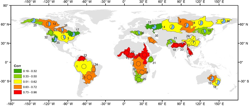
The 35 largest (by area) river basins from the total runoff integrating pathway (TRIP) database [73] (see Figure 1) were selected to demonstrate the TC-based and BP detection methods. Climates of the selected basins, which are classified using the mean annual aridity index [74], are humid (H) (22 basins), semi-humid (SH) (2 basins), semi-arid (SA) (10 basins), and arid (A) (1 basin) (4th and 5th columns in Table 1). The percentage of irrigated area in each basin is listed in the last column of Table 1.
4.1. EMD Results
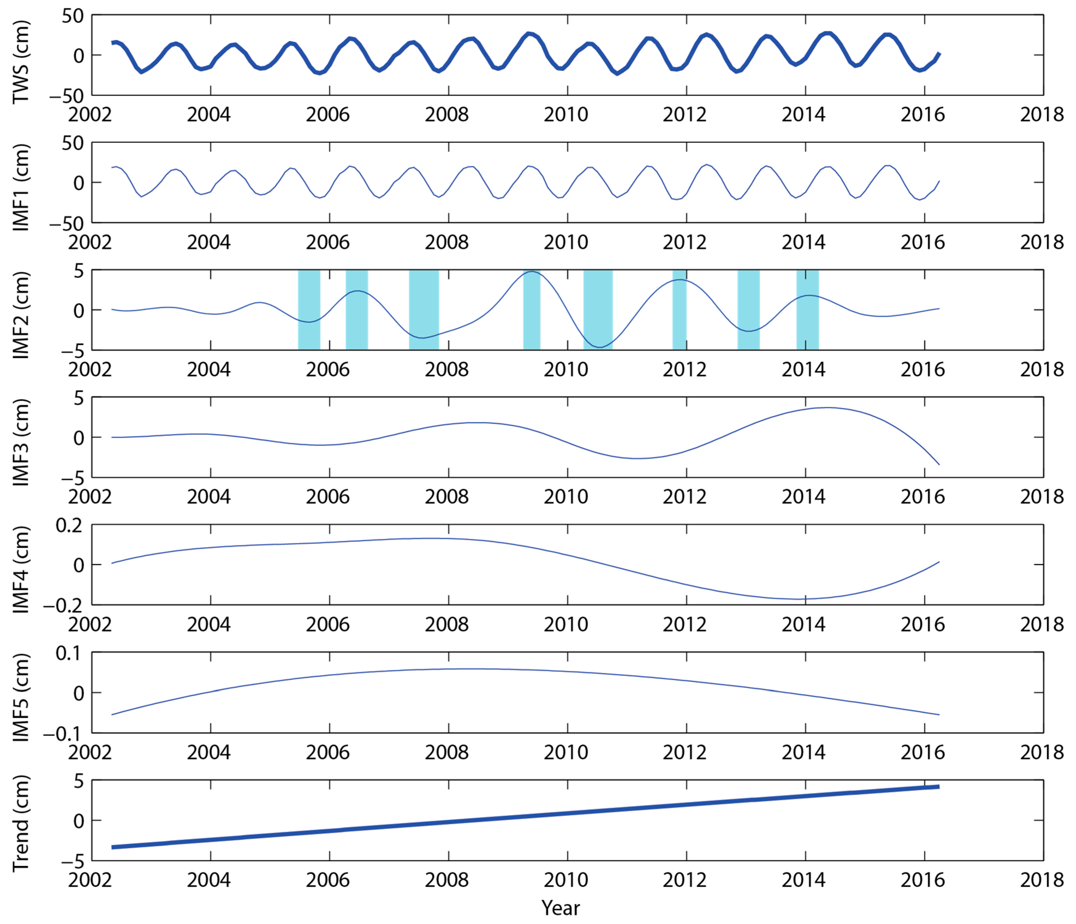
EMD was first applied to the basin-averaged TWSA time series obtained using the CSR-M GRACE product. In Figure 2, results for the Amazon River basin are shown. The EMD analysis shows an upward linear trend over the study period (bottom panel). The frequencies of 5 IMFs decrease from the top to bottom. IMF1 is the dominant mode in signal amplitude, consisting of a sinusoid varying at annual cycle (mean period = 12 months). IMF2 is at approximately biennial scale (mean period = 28 months). IMF3 represents a longer-term, interannual oscillation (mean period = 56 months). IMF4 and IMF5 are similar, both representing small-amplitude, interdecadal oscillations; thus, they should be combined according to the guidance in [70] (p. 12). In the following discussion, we put the relevant references after all identified events for ease of interpretation and confirmation. We also consulted the online international disasters database, EM-DATA [75], for flood and drought events.
The extrema of IMF2 correspond well to the known hydrologic extremes occurred at the Amazon River basin, including the extreme drought of 2005 [76] and 2010 [40,43], and the extreme floods in 2009 [77], austral summer in 2011–2012 [78], and austral summer of 2013–2014 [79]. The less discussed wet year 2006 and dry year 2007 [43] are also discernable. Thus, in this case IMF2 is the “extreme indicator” IMF. Note that the index of extreme indicator IMF may vary for other basins, depending on the mean return period.
Amazon River basin is known for its strong cyclic patterns. So, can we find similar indicator IMFs for other basins?
Figure 3a–d show the indicator IMFs identified for four additional large river basins, namely, Mississippi (H), Nile (SA), Zambezi (SH), and Murray Darling (SA). Different from the Amazon River basin, all basins show strong nonstationarity during the study period (solid TWSA lines in Figure 3).
In the Mississippi River basin, the indicator IMF (dashed line) identifies the extreme U.S. midwest flood in 2011 [12], the extreme drought in 2012 [41]; also, the dry event in 2002–2003, the hurricane-related wet year 2005, wet event in the beginning of 2008, wet year 2013–2014 can be observed [75,80].
For the Nile River basin, the indicator IMF reveals major dry events in 2003, 2005, 2006, 2009, 2011, some of which were related to ENSO; the wet events in 2003, 2005, 2007 were also documented [75,81].
In the case of Zambezi River basin, which is known for its strong annual storage variations [82], the shape of indicator IMF is more interesting and is dominated by a long extreme drought occurred in eastern Africa in 2003–2006 (separated by a wet event in 2004), followed by a sudden increase in 2007 [83]; afterward, the region encountered flood events almost annually between 2007 and 2014 [75]. The Murray Darling basin in Australia experienced a prolonged drought period [84] that ended in 2010; the recent wet events in 2012 and 2014–2015, and dry events in 2011, end of 2013, and 2015 may also be seen [75].
The full set of IMFs for each basin are plotted in SI Part B, which suggest that in all basins except Mississippi a nonlinear EMD trend exists that appeared to be relatively flat between 2002 and 2009/2010 and then started to increase after that.
The mean periods for all basins are listed in Table 1, which generally range from two to three years. This information was then used to derive the h values required for the following BP analyses.
4.2. TC and BP Results
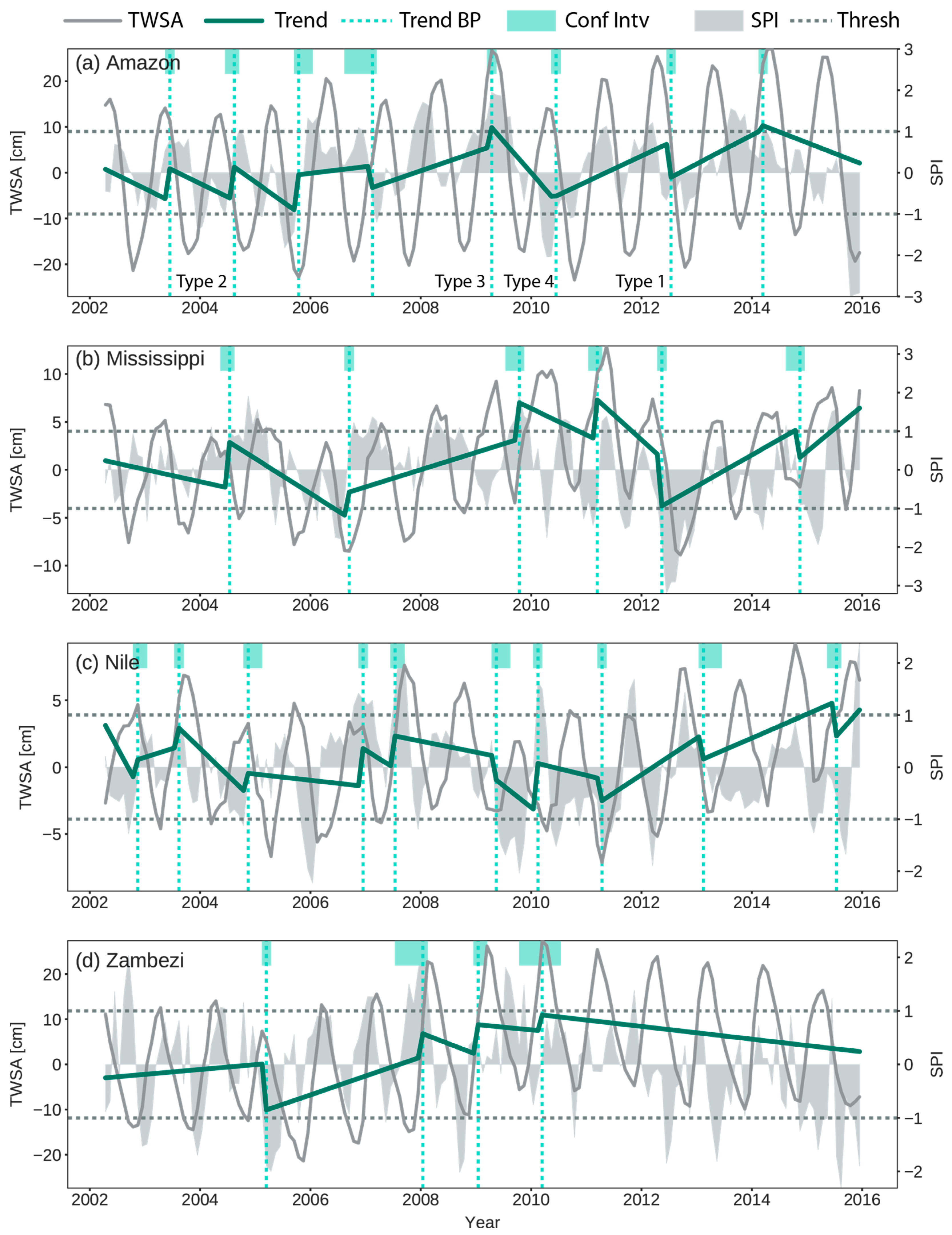
The BP and TC-based methods were performed using the same basin-averaged TWSA time series. Here we showcase the results for four major river basins, Amazon, Mississippi, Nile, and Zambezi.
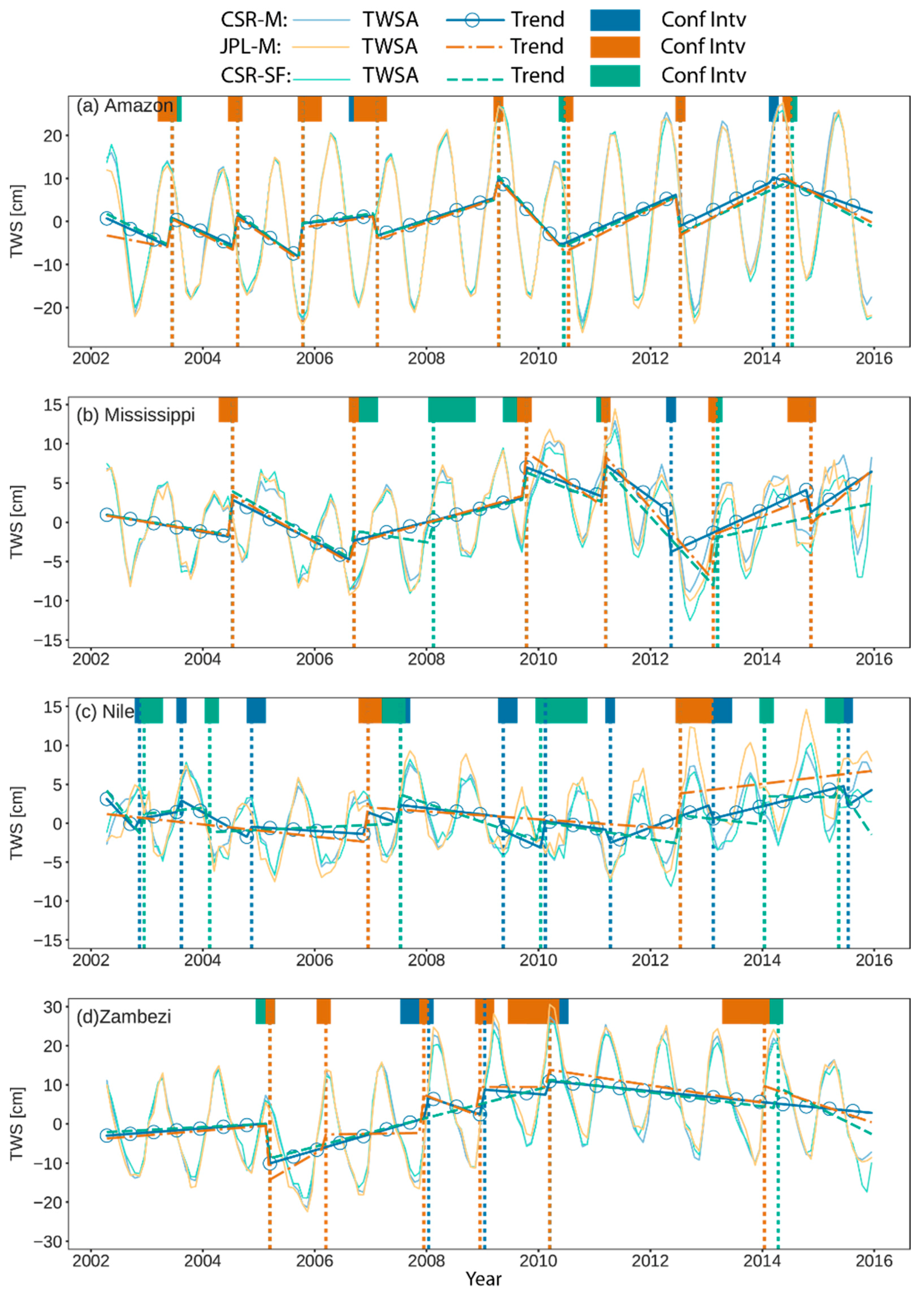
Figure 4a–d show BPs detected in each of the four basins. On the left axis of each subplot, the BFAST trend (dark green solid line) is overlaid on the original TWSA data (dark gray solid line), together with BP times (vertical dotted line) and the associated 95% confidence intervals (shaded green boxes near the top of each subplot). For comparison, monthly SPI3 series is plotted on the right axis (filled line plots) and its ±1 thresholds are shown with horizontal, dotted lines in gray.
The BP detection procedure seeks to optimally divide the whole time series into multiple short periods, separated by abrupt changes (BPs). In our study, we found that all BPs are related to abrupt changes in the trend. For the Amazon River basin, the major drought in 2005 was part of a declining trend that started in late 2004 and was only interrupted by the wet year in 2006. Similarly, the extreme drought in 2010 was part of a sharp declining trend that started since the end of extreme Amazon flood in 2009. Similar to the extreme indicator IMFs resulting from the EMD, BPs are related to local extrema in a time series—the number of BPs detected agrees with the number of extrema in the extreme indicator IMF. Unlike the indicator IMFs, however, BP detection reveals not only abrupt changes, but also the actual trends in between. The magnitudes of these short-term trends reflect the rate of decline or recovery. In this case, the transition from the extreme wet 2009 to extreme dry 2010 makes the trend in 2009–2010 the steepest decline. In many cases, the abrupt changes may also be accompanied by sharp jumps in the trend to adapt to a new short-term regime. For instance, the positive jump at the end of 2005 drought, the positive jump related to 2009 flood, and the negative jump related to the dry event in 2013.
Using the BP classification scheme mentioned in Section 3, we can see examples of all four types of abrupt changes in Figure 4a. Specifically, the 2003–2005 dry period was interrupted by a small-magnitude wet event in 2004, making it a Type 2 event preceded and succeeded by negative trends. The 2010–2014 wet period was interrupted by a dry event in 2012, making the BP a Type 1 event that was both preceded and succeeded by positive trends. The 2009 flood was a Type 3 event (+/−), while the 2010 extreme drought was a Type 4 event (−/+).
For the Mississippi River basin, notable BPs are related to a wet event in 2004, drought period in 2005–2006, extreme flood in 2011, and a severe drought that started in 2012. Like in the case of Amazon River basin during 2009–2010, the short period 2010–2012 included a massive flood followed by a drought event. The 2012 Central U.S. flash drought impacted major agricultural areas across the region and had a severity comparable to historical extreme droughts during the 1930s and 1950s [85,86]. The 2012 BP is thus accompanied by a sharp drop in TWSA magnitude. A major difference between Figure 4b and its corresponding IMF (Figure 3a) is in the period 2008–2010, where the IMF showed a wet event in 2008 and two dry events in 2007 and 2009, while the BP results suggested a positive trend in the period. This phenomenon may be attributed to the mixing of signals by the harmonic seasonal component assumed in BFAST.
Both the Nile River basin and Zambezi River basin are characterized by high-frequency precipitation and TWSA variations. In Nile River basin, major BPs corresponded to 2003, 2007, 2010 wet events, and 2005, 2009, 2011 dry events. In Zambezi River basin, a severe drought occurred in 2005, followed by a 3-year wet period until 2008, and then a downward trend continued after 2010. In these cases, the BP algorithm detected the major events, but also missed some smaller-magnitude, short-term events, for example, the sharp downward spike in late 2005 in Nile River basin. We note that the indicator IMF for the Nile River basin (Figure 3b) detected the 2005 event. Similarly, the indicator IMF for the Zambezi River basin (Figure 3c) also identified the short-term events happened in the beginning of 2012 and in late 2003.
Figure 5a–d provide results obtained using the TC-based method. The normalized TWSA index values were smoothed using the 3-month moving average. Overall, the TC method seems to capture some SPI extreme events well, including their durations, for example, the 2005, 2010 droughts and 2009 flood in the Amazon River basin; the 2009 flood and 2012 midwest drought in the Mississippi River basin; and the beginning of extreme dry period in the Zambezi River basin in 2005. However, some event durations were significantly exaggerated, as compared to SPI. For example, the Mississippi 2005–2009 drought period and the 2005–2008 Zambezi drought.
It may be argued that TWS takes longer to recover to its normal conditions than SPI [41]; however, differences between TWSA extremes and rainfall anomalies need to be clarified and quantified, at least in terms of the event timings. To address this latter issue, we applied the ECA method to quantify concurrence between SPI anomalies and TWSA by considering the inherent lags identified during the following correlation analysis.
4.3. ECA Results
Lagged correlations between the cumulative rainfall residuals and CSR-M TWSA were quantified using the method described under Section 3. The lags for all 35 basins are already shown in Figure 1 (normalized by 12 months), which are binned into different color groups according to the maximum correlation. The actual numerical values are reported under the 7th and 8th columns in Table 1. The lagged correlation between cumulative P residuals and TWSA ranges from 0.19 (Colorado River basin) to 0.96 (Chari basin), and all correlation values reported here are significant with a p-value less than 0.02. About half of the 35 basins show no lags between cumulative P residuals and TWSA. The maximum lag is up to nine months (Volga River basin). In general, non-zero lags were observed for north hemisphere, high-latitude basins, while zero lags were identified for basins in tropical climate regions. Human water management activities may be responsible for the relatively long lag (seven months) and low correlation obtained for the Colorado River basin.
For event extraction using the TC-based method, we used ±1 as thresholds. Similarly, the rainfall anomalies were also obtained by using thresholds ±1 on SPI, as mentioned in Section 2. While SPI cutoff values are linked to different levels of event severity, no such standard seems to exist for TWSA extreme events. Previously, Humphrey et al. [39] used an absolute water storage deficit value of 30 mm to extract drought events, while Thomas et al. [41] defined droughts as events when water storage deficits last three months or longer. Here, the thresholds for the normalized TWSA were chosen so that TC methods would include similar events as SPI.
For the BP method, times of abrupt changes (BPs) were used to form event series. The time lags found in the aforementioned correlation analysis were used to define the width of sliding window between TWSA and SPI for both TC and BP methods in ECA calculations. The final results of ECA are reported in Table 1.
The ECA results reported in Table 1 (9th column) suggest that almost all basin-scale abrupt changes (BPs) are perfectly related to some antecedent SPI events. Only Congo and Nile river basins have values less than 1. In contrast, events extracted using the climatology-based TC method gave much lower coincidence rates (10th column in Table 1) over many river basins. Relatively low TC coincidence rates are generally found in north hemisphere, high-latitude basins, such as in St. Lawrence (0.55) and Yukon (0.52); in heavily managed basins, such as Colorado basin (0.58); or in semiarid areas, such as Niger (0.56). These results indicate that BP detection method achieved better accuracy in uncovering extreme events, as relative to SPI events, than the TC method.
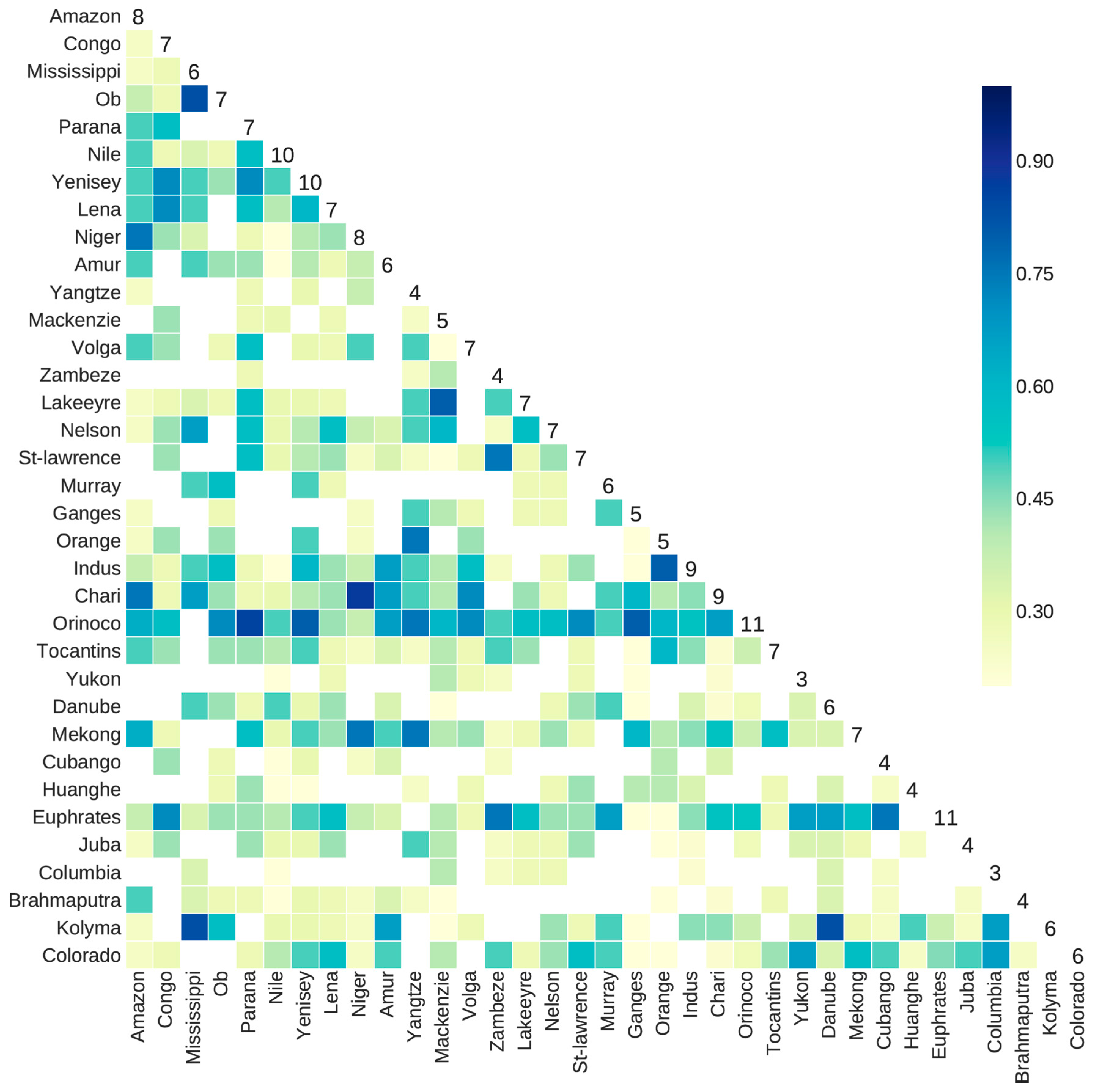
At last, we quantified the pairwise, coincidence rates of TWSA extreme events for all 35 river basins. For each river basin, event coincidence rates were calculated between that basin and all other basins. The event series were formed by using results of the BP detection method. The results were used to build a coincidence matrix as shown in Figure 6. The meaning of this BP coincidence matrix is similar to the correlation-based TWSA connectivity map, which measures how TWS in different basins tend to co-vary [87,88]. The difference is that a nonparametric ECA measure is used in our analyses.
Figure 6 suggests that geographically close basins (e.g., Yenisei/Ob/Lena and Niger/Chari) generally show high coincidence rates. Basins that are affected by similar climatic circulation forcing (e.g., Orinoco/Parana, Indus/Orange) also show high coincidence in BP events. Other cases, such as the relatively high coincidence rate between the high-latitude Kolyma and Mississippi basin is intriguing. Similar patterns could be observed from the connectivity map in Sun et al. (Figure 2, [88]). Interestingly, the Orinoco River basin that is north of the Amazon River basin seems to have strong linkage with a large number of river basins. Many other basins, such as the Huanghe River basin in North China Plain, Yukon, Brahmaputra, and Murray–Darling are relatively disconnected with other basins.
Our basin-scale analyses show that the BP method provides a more robust tool for identifying hydrologic extremes. A consistent causal relationship (in the ECA sense) was found between BP and SPI events for river basins considered here. On the other hand, the event coincidence rates derived using the TC method are mixed due to the limited length of GRACE records.
5. Discussion
In this study, two non-parametric methods, EMD and ECA were used to understand dynamics of TWSA extremes. Overall, our EMD exploratory analysis results suggest that the extreme indicator IMF observed for the Amazon River basin (Figure 2), which exhibits strong seasonality, is not fortuitous. In fact, we were able to identify and subsequently corroborate an appropriate extreme indicator IMF for all major basins considered here (Table 1), indicating the usefulness of EMD as a preliminary analysis tool for isolating the inherent temporal scale related to TWSA extremes. As far as we know, only one previous study [44] had tried to quantify return periods of TWSA events by using GRACE climatology and the traditional frequency analysis (e.g., deriving one-in-five-year probability of anomalously high TWSA with ~10 years of data). A main strength of the EMD analysis is that it is entirely data driven and is not limited by the stationarity assumption. The observation that the mean return period of TWSA extremes ranges from 15 to 42 months for all basins studied (Table 1) is an interesting finding and warrants further studies for predictive analyses.
The event coincidence metric provides a simple measure for quantifying causal relationships between events. The event coincidence between P and TWSA events was found to be 1.0 for most of the river basins, regardless of the climate regime, suggesting the dominant role of precipitation in driving TWS dynamics [87].
As mentioned in Section 2.1, TWSA may be affected by uncertainty in data processing and inherent measurement errors. A standard approach in the research community has been comparing multiple GRACE products. Thus, we repeated the same basin-scale BP analyses done in Section 4.2, but using the scaled SH product from CSR (CSR-SF, SF is short for scaled factor) and the JPL-M mascon solution. The results are compared in Figure 7.
Overall, Figure 7 suggests that abrupt changes detected using the three different GRACE products are generally in agreement with each other. For the Amazon River basin, all three products gave very similar results. Slight differences were noticed only around the 2010 extreme drought and the 2014 wet event. For the Mississippi River basin, the main difference is that both JPL-M and CSR-SF missed the onset of the severe 2012 drought and only gave a BP towards early 2013. CSR-SF was the only product that detected the short-term meteorological drought happened in early 2008. On the other hand, CSR-SF did not detect the BP that happened in late 2014 that corresponded to a dry event. For the Nile River basin, the three GRACE products showed more discrepancies than in other cases, which may be attributed to the differences in the magnitudes of TWSA time series—the semiarid nature of Nile River basin and strong annual variability makes it more difficult to track TWS changes, leading to larger uncertainty in various GRACE products. For Zambezi River basin, CSR-M and JPL-M show similar BPs, but CSR-SF was not sensitive to many small-scale events between 2006 and 2014.
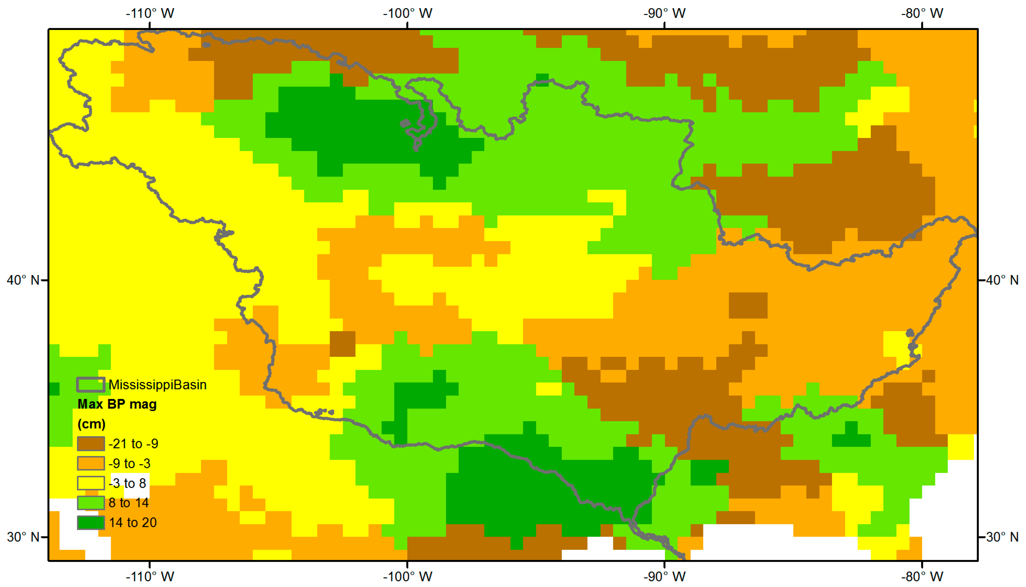
In this study, we mainly focused on analyzing the basin-averaged TWSA time series. The same EMD-assisted BP analysis procedure may be applied at the intra-basin scale to investigate the spatial distribution of TWSA extremes. As an illustration, Figure 8 shows the maximum value (in absolute magnitude) of all BPs detected at each grid block for the Mississippi River basin. The negative maximum BPs in the southeast part (Arkansas-White-River and Lower Mississippi) of the basin are related to droughts in 2005, whereas the positive maximum BPs observed in the northwest part are related to a wet season in the spring of 2013 that ended the 2012 flash drought at the region.
6. Conclusions
A comparative study was performed on the skill of climatology-based (TC) and breakpoint (BP) analyses for detecting hydrologic extremes over the world’s 35 largest river basins by using GRACE TWSA products. The empirical mode decomposition (EMD) was used as a preliminary step before BP analyses to uncover the mean return period of extreme events for each basin. The TC method requires access to stable long-term climatology and uses a pre-defined threshold to identify anomalous events, whereas the EMD-assisted BP method iteratively identifies the optimal number, time, magnitude, and type of BPs in a time series with little subjectivity. Our comparison results show that the BP method explains the occurrences of hydrologic extremes better in all basins examined, and correlate well with precipitation anomalies.
The potential merit of TWSA over forcing-based index (SPI) or simple water-budget based (e.g., PDSI) indices for monitoring large-scale, hydrologic extremes has been demonstrated in previous studies [18,35,41]. This study further demonstrates that EMD-assisted BP detection method provides an alternative and more robust tool for detecting hydrologic extremes without being restricted by the limited GRACE climatology (14 years for the study period) and the everlasting stationarity question.
Currently GRACE products are limited by their spatial and temporal resolution. Recent studies demonstrate the feasibility of downscaling GRACE data spatially and temporally using data assimilation and statistical approaches, potentially extending the applicability of BP analysis to smaller regions [89,90,91,92] and shorter timescales [93,94]. In the future, these new data processing techniques can be combined with EMD-assisted BP analysis presented in this study to detect the onset of extreme events.
Supplementary Materials
The following are available online at www.mdpi.com/2072-4292/9/12/1287/s1, SI Part A; SI Part B.
Acknowledgments
The GRACE solutions used in this study are downloadable from JPL (www.grace.jpl.nasa.gov) and UT CSR site (http://www.csr.utexas.edu/grace/). GLDAS data were downloaded from NASA GES DISC (http://disc.sci.gsfc.nasa.gov/uui/datasets?keywords=GLDAS). TRMM data are available from NASA mirador data portal, https://mirador.gsfc.nasa.gov. Data analyses were performed using R and Python scripts. A. Y. Sun and B. R. Scanlon were partially supported by funding from Jackson School of Geosciences, UT Austin. A. AghaKouchak was partially supported by the National Aeronautics and Space Administration (NASA) Award No. NNX15AC27G. Z. Zhang was supported by the National Natural Science Foundation of China (Grant No. 41674085). The authors are grateful to the AE, the Guest Editor (Di Long), and two anonymous reviewers for their constructive comments.
Author Contributions
A.Y.S. conceived the original experiments; B.R.S. and A.A. helped improve experimental design; Z.Z. provided basin averaged data processing; A.Y.S. conducted the experiments; all contributed to data analyses, result interpretation, and writing of the paper.
Conflicts of Interest
The authors declare no conflict of interest.
Abbreviations
| BP | Breakpoint |
| CSR | Center for Space Research |
| EMD | Empirical mode decomposition |
| ECA | Event coincidence analysis |
| GLDAS | Global Land Data Assimilation System |
| GPCP | Global Precipitation Climatology Project |
| GRACE | Gravity Recovery and Climate Experiment |
| IMF | Intrinsic mode function |
| Mascon | Mass concentration |
| JPL | Jet Propulsion Laboratory |
| LSM | Land surface model |
| PDSI | Palmer Drought Severity Index |
| SH | Spherical harmonic |
| SPI | Standardized Precipitation Index |
| TC | TWSA-climatology |
| TRMM | Tropical Rainfall Measuring Mission |
| TWS | Total water storage |
| TWSA | total water storage anomalies |
References
- Diffenbaugh, N.S.; Scherer, M. Observational and model evidence of global emergence of permanent, unprecedented heat in the 20th and 21st centuries. Clim. Chang. 2011, 107, 615–624. [Google Scholar] [CrossRef] [PubMed]
- D’Odorico, P.; Laio, F.; Ridolfi, L. Does globalization of water reduce societal resilience to drought? Geophys. Res. Lett. 2010, 37. [Google Scholar] [CrossRef]
- Coumou, D.; Rahmstorf, S. A decade of weather extremes. Nat. Clim. Chang. 2012, 2, 491–496. [Google Scholar] [CrossRef]
- Donat, M.G.; Lowry, A.L.; Alexander, L.V.; O’Gorman, P.A.; Maher, N. More extreme precipitation in the world’s dry and wet regions. Nat. Clim. Chang. 2016, 508–513. [Google Scholar] [CrossRef]
- Mazdiyasni, O.; AghaKouchak, A. Substantial increase in concurrent droughts and heatwaves in the United States. Proc. Natl. Acad. Sci. USA 2015, 112, 11484–11489. [Google Scholar] [CrossRef] [PubMed]
- Milly, P.C.D.; Wetherald, R.T.; Dunne, K.; Delworth, T.L. Increasing risk of great floods in a changing climate. Nature 2002, 415, 514–517. [Google Scholar] [CrossRef] [PubMed]
- Zhang, X.; Alexander, L.; Hegerl, G.C.; Jones, P.; Tank, A.K.; Peterson, T.C.; Trewin, B.; Zwiers, F.W. Indices for monitoring changes in extremes based on daily temperature and precipitation data. Wiley Interdiscip. Rev. Clim. Chang. 2011, 2, 851–870. [Google Scholar] [CrossRef]
- Hao, Z.; Singh, V.P. Drought characterization from a multivariate perspective: A review. J. Hydrol. 2015, 527, 668–678. [Google Scholar] [CrossRef]
- Sadegh, M.; Ragno, E.; AghaKouchak, A. Multivariate copula analysis toolbox (mvcat): Describing dependence and underlying uncertainty using a Bayesian framework. Water Resour. Res. 2017, 53, 5166–5183. [Google Scholar] [CrossRef]
- Riegger, J.; Tourian, M. Characterization of runoff-storage relationships by satellite gravimetry and remote sensing. Water Resour. Res. 2014, 50, 3444–3466. [Google Scholar] [CrossRef]
- Reager, J.; Famiglietti, J. Global terrestrial water storage capacity and flood potential using GRACE. Geophys. Res. Lett. 2009, 36. [Google Scholar] [CrossRef]
- Reager, J.; Thomas, B.; Famiglietti, J. River basin flood potential inferred using GRACE gravity observations at several months lead time. Nat. Geosci. 2014, 7, 588–592. [Google Scholar] [CrossRef]
- Rodell, M.; Velicogna, I.; Famiglietti, J.S. Satellite-based estimates of groundwater depletion in India. Nature 2009, 460, 999–1002. [Google Scholar] [CrossRef] [PubMed]
- Sun, A.Y.; Green, R.; Swenson, S.; Rodell, M. Toward calibration of regional groundwater models using GRACE data. J. Hydrol. 2012, 422, 1–9. [Google Scholar] [CrossRef]
- Zhao, M.; Velicogna, I.; Kimball, J.S. Satellite observations of regional drought severity in the continental United States using GRACE-based terrestrial water storage changes. J. Clim. 2017, 30, 6297–6308. [Google Scholar] [CrossRef]
- Chen, J.L.; Famigliett, J.S.; Scanlon, B.R.; Rodell, M. Groundwater storage changes: Present status from GRACE observations. In Remote Sensing and Water Resources; Cazenave, A., Champollion, N., Benveniste, J., Chen, J., Eds.; Springer International Publishing: Berlin, Germany, 2016; pp. 207–227. [Google Scholar]
- Ramillien, G.; Famiglietti, J.S.; Wahr, J. Detection of continental hydrology and glaciology signals from GRACE: A review. Surv. Geophys. 2008, 29, 361–374. [Google Scholar] [CrossRef]
- Houborg, R.; Rodell, M.; Li, B.; Reichle, R.; Zaitchik, B.F. Drought indicators based on model-assimilated gravity recovery and climate experiment (GRACE) terrestrial water storage observations. Water Resour. Res. 2012, 48. [Google Scholar] [CrossRef]
- Zhao, M.; Velicogna, I.; Kimball, J.S. A global gridded dataset of grace drought severity index for 2002–14: Comparison with PDSI and SPEI and a case study of the Australia millennium drought. J. Hydrometeorol. 2017, 18, 2117–2129. [Google Scholar] [CrossRef]
- Syed, T.H.; Famiglietti, J.; Chen, J.; Rodell, M.; Seneviratne, S.; Viterbo, P.; Wilson, C. Total basin discharge for the Amazon and Mississippi river basins from GRACE and a land-atmosphere water balance. Geophys. Res. Lett. 2005, 32. [Google Scholar] [CrossRef]
- Scanlon, B.R.; Zhang, Z.; Reedy, R.C.; Pool, D.R.; Save, H.; Long, D.; Chen, J.; Wolock, D.M.; Conway, B.D.; Winester, D. Hydrologic implications of grace satellite data in the Colorado River basin. Water Resour. Res. 2015, 51, 9891–9903. [Google Scholar] [CrossRef]
- Yeh, P.J.F.; Swenson, S.; Famiglietti, J.; Rodell, M. Remote sensing of groundwater storage changes in Illinois using the Gravity Recovery and Climate Experiment (GRACE). Water Resour. Res. 2006, 42. [Google Scholar] [CrossRef]
- Sun, A.Y.; Green, R.; Rodell, M.; Swenson, S. Inferring aquifer storage parameters using satellite and in situ measurements: Estimation under uncertainty. Geophys. Res. Lett. 2010, 37. [Google Scholar] [CrossRef]
- Richey, A.S.; Thomas, B.F.; Lo, M.H.; Famiglietti, J.S.; Swenson, S.; Rodell, M. Uncertainty in global groundwater storage estimates in a total groundwater stress framework. Water Resour. Res. 2015, 51, 5198–5216. [Google Scholar] [CrossRef] [PubMed]
- Long, D.; Longuevergne, L.; Scanlon, B.R. Uncertainty in evapotranspiration from land surface modeling, remote sensing, and GRACE satellites. Water Resour. Res. 2014, 50, 1131–1151. [Google Scholar] [CrossRef] [Green Version]
- Rodell, M.; Famiglietti, J.S.; Chen, J.L.; Seneviratne, S.I.; Viterbo, P.; Holl, S.; Wilson, C.R. Basin scale estimates of evapotranspiration using GRACE and other observations. Geophys. Res. Lett. 2004, 31. [Google Scholar] [CrossRef]
- Castle, S.L.; Reager, J.T.; Thomas, B.F.; Purdy, A.J.; Lo, M.H.; Famiglietti, J.S.; Tang, Q. Remote detection of water management impacts on evapotranspiration in the Colorado River basin. Geophys. Res. Lett. 2016, 43, 5089–5097. [Google Scholar] [CrossRef]
- Richey, A.S.; Thomas, B.F.; Lo, M.H.; Reager, J.T.; Famiglietti, J.S.; Voss, K.; Swenson, S.; Rodell, M. Quantifying renewable groundwater stress with GRACE. Water Resour. Res. 2015, 51, 5217–5238. [Google Scholar] [CrossRef] [PubMed]
- Frappart, F.; Ramillien, G.; Biancamaria, S.; Mognard, N.M.; Cazenave, A. Evolution of high-latitude snow mass derived from the GRACE gravimetry mission (2002–2004). Geophys. Res. Lett. 2006, 33. [Google Scholar] [CrossRef] [Green Version]
- Schmidt, R.; Flechtner, F.; Meyer, U.; Neumayer, K.-H.; Dahle, C.; König, R.; Kusche, J. Hydrological signals observed by the GRACE satellites. Surv. Geophys. 2008, 29, 319–334. [Google Scholar] [CrossRef]
- Scanlon, B.R.; Longuevergne, L.; Long, D. Ground referencing GRACE satellite estimates of groundwater storage changes in the California Central Valley, USA. Water Resour. Res. 2012, 48. [Google Scholar] [CrossRef] [Green Version]
- Xia, Y.; Mocko, D.; Huang, M.; Li, B.; Rodell, M.; Mitchell, K.E.; Cai, X.; Ek, M.B. Comparison and assessment of three advanced land surface models in simulating terrestrial water storage components over the United States. J. Hydrometeorol. 2017, 18, 625–649. [Google Scholar] [CrossRef]
- Khandu, K.; Forootan, E.; Schumacher, M.; Awange, J.L.; Müller Schmied, H. Exploring the influence of precipitation extremes and human water use on total water storage (TWS) changes in the Ganges-Brahmaputra-Meghna river basin. Water Resour. Res. 2016. [Google Scholar] [CrossRef]
- Crowley, J.W.; Mitrovica, J.X.; Bailey, R.C.; Tamisiea, M.E.; Davis, J.L. Land water storage within the Congo basin inferred from GRACE satellite gravity data. Geophys. Res. Lett. 2006. [Google Scholar] [CrossRef]
- Long, D.; Scanlon, B.R.; Longuevergne, L.; Sun, A.Y.; Fernando, D.N.; Himanshu, S. GRACE satellites monitor large depletion in water storage in response to the 2011 drought in Texas. Geophys. Res. Lett. 2013, 40, 3395–3401. [Google Scholar] [CrossRef] [Green Version]
- AghaKouchak, A.; Farahmand, A.; Melton, F.; Teixeira, J.; Anderson, M.; Wardlow, B.; Hain, C. Remote sensing of drought: Progress, challenges and opportunities. Rev. Geophys. 2015, 53, 452–480. [Google Scholar] [CrossRef]
- Yirdaw, S.Z.; Snelgrove, K.R.; Agboma, C.O. GRACE satellite observations of terrestrial moisture changes for drought characterization in the Canadian prairie. J. Hydrol. 2008, 356, 84–92. [Google Scholar] [CrossRef]
- Abelen, S.; Seitz, F.; Abarca-del-Rio, R.; Güntner, A. Droughts and floods in the La Plata basin in soil moisture data and GRACE. Remote Sens. 2015, 7, 7324–7349. [Google Scholar] [CrossRef]
- Humphrey, V.; Gudmundsson, L.; Seneviratne, S.I. Assessing global water storage variability from GRACE: Trends, seasonal cycle, subseasonal anomalies and extremes. Surv. Geophys. 2016, 37, 357–395. [Google Scholar] [CrossRef] [PubMed]
- Maeda, E.E.; Kim, H.; Aragão, L.E.; Famiglietti, J.S.; Oki, T. Disruption of hydroecological equilibrium in southwest Amazon mediated by drought. Geophys. Res. Lett. 2015, 42, 7546–7553. [Google Scholar] [CrossRef]
- Thomas, A.C.; Reager, J.T.; Famiglietti, J.S.; Rodell, M. A GRACE-based water storage deficit approach for hydrological drought characterization. Geophys. Res. Lett. 2014, 41, 1537–1545. [Google Scholar] [CrossRef]
- Long, D.; Shen, Y.; Sun, A.Y.; Hong, Y.; Longuevergne, L.; Yang, Y.; Li, B.; Chen, L. Drought and flood monitoring for a large karst plateau in southwest China using extended GRACE data. Remote Sens. Environ. 2014, 155, 145–160. [Google Scholar] [CrossRef]
- Frappart, F.; Ramillien, G.; Ronchail, J. Changes in terrestrial water storage versus rainfall and discharges in the Amazon basin. Int. J. Climatol. 2013, 33, 3029–3046. [Google Scholar] [CrossRef] [Green Version]
- Kusche, J.; Eicker, A.; Forootan, E.; Springer, A.; Longuevergne, L. Mapping probabilities of extreme continental water storage changes from space gravimetry. Geophys. Res. Lett. 2016, 43, 8026–8034. [Google Scholar] [CrossRef]
- Cheng, L.; AghaKouchak, A.; Gilleland, E.; Katz, R.W. Non-stationary extreme value analysis in a changing climate. Clim. Chang. 2014, 127, 353–369. [Google Scholar] [CrossRef]
- Gilleland, E.; Katz, R.W. New software to analyze how extremes change over time. Eos Trans. Am. Geophys. Union 2011, 92, 13–14. [Google Scholar] [CrossRef]
- Katz, R.W. Statistical methods for nonstationary extremes. In Extremes in a Changing Climate; Springer: Berlin, Germany, 2013; pp. 15–37. [Google Scholar]
- Mann, H.B. Nonparametric tests against trend. Econom. J. Econom. Soc. 1945, 245–259. [Google Scholar] [CrossRef]
- Yue, S.; Wang, C. The mann-kendall test modified by effective sample size to detect trend in serially correlated hydrological series. Water Resour. Manag. 2004, 18, 201–218. [Google Scholar] [CrossRef]
- Amiri, A.; Allahyari, S. Change point estimation methods for control chart postsignal diagnostics: A literature review. Qual. Reliab. Eng. Int. 2012, 28, 673–685. [Google Scholar] [CrossRef]
- Lund, R.; Wang, X.L.; Lu, Q.Q.; Reeves, J.; Gallagher, C.; Feng, Y. Changepoint detection in periodic and autocorrelated time series. J. Clim. 2007, 20, 5178–5190. [Google Scholar] [CrossRef]
- Chandola, V.; Banerjee, A.; Kumar, V. Anomaly detection: A survey. ACM Comput. Surv. 2009, 41. [Google Scholar] [CrossRef]
- Verbesselt, J.; Hyndman, R.; Zeileis, A.; Culvenor, D. Phenological change detection while accounting for abrupt and gradual trends in satellite image time series. Remote Sens. Environ. 2010, 114, 2970–2980. [Google Scholar] [CrossRef]
- Verbesselt, J.; Zeileis, A.; Herold, M. Near real-time disturbance detection using satellite image time series. Remote Sens. Environ. 2012, 123, 98–108. [Google Scholar] [CrossRef]
- Huang, N.E.; Shen, Z.; Long, S.R.; Wu, M.C.; Shih, H.H.; Zheng, Q.; Yen, N.-C.; Tung, C.C.; Liu, H.H. The Empirical Mode Decomposition and the Hilbert Spectrum for Nonlinear and Non-Stationary Time Series Analysis. Proc. R. Soc. Lond. A Math. Phys. Eng. Sci. 1998, 454, 903–995. [Google Scholar] [CrossRef]
- Wu, Z.; Huang, N.E. A study of the characteristics of white noise using the empirical mode decomposition method. Proc. R. Soc. Lond. A Math. Phys. Eng. Sci. 2004, 1597–1611. [Google Scholar] [CrossRef]
- Chen, C.-F.; Lai, M.-C.; Yeh, C.-C. Forecasting tourism demand based on empirical mode decomposition and neural network. Knowl. Based Syst. 2012, 26, 281–287. [Google Scholar] [CrossRef]
- Zhang, X.; Lai, K.K.; Wang, S.-Y. A new approach for crude oil price analysis based on empirical mode decomposition. Energy Econ. 2008, 30, 905–918. [Google Scholar] [CrossRef]
- Lee, T.; Ouarda, T. Prediction of climate nonstationary oscillation processes with empirical mode decomposition. J. Geophys. Res. Atmos. 2011, 116. [Google Scholar] [CrossRef]
- Rodell, M.; Houser, P.; Jambor, U.; Gottschalck, J.; Mitchell, K.; Meng, C.; Arsenault, K.; Cosgrove, B.; Radakovich, J.; Bosilovich, M. The global land data assimilation system. Bull. Am. Meteorol. Soc. 2004, 85, 381–394. [Google Scholar] [CrossRef]
- Landerer, F.W.; Swenson, S.C. Accuracy of scaled GRACE terrestrial water storage estimates. Water Resour. Res. 2012, 48. [Google Scholar] [CrossRef]
- Long, D.; Longuevergne, L.; Scanlon, B.R. Global analysis of approaches for deriving total water storage changes from GRACE satellites. Water Resour. Res. 2015, 51, 2574–2594. [Google Scholar] [CrossRef] [Green Version]
- Watkins, M.M.; Wiese, D.N.; Yuan, D.N.; Boening, C.; Landerer, F.W. Improved methods for observing Earth’s time variable mass distribution with GRACE using spherical cap mascons. J. Geophys. Res. Solid Earth 2015, 120, 2648–2671. [Google Scholar] [CrossRef]
- Save, H.; Bettadpur, S.; Tapley, B.D. High-resolution CSR GRACE mascons. J. Geophys. Res. Solid Earth 2016, 121, 7547–7569. [Google Scholar] [CrossRef]
- Scanlon, B.R.; Zhang, Z.; Save, H.; Wiese, D.N.; Landerer, F.W.; Long, D.; Longuevergne, L.; Chen, J. Global evaluation of new GRACE mascon products for hydrologic applications. Water Resour. Res. 2017, 52, 9412–9429. [Google Scholar] [CrossRef]
- Huffman, G.J.; Bolvin, D.T.; Nelkin, E.J.; Wolff, D.B.; Adler, R.F.; Gu, G.; Hong, Y.; Bowman, K.P.; Stocker, E.F. The TRMM multisatellite precipitation analysis (TMPA): Quasi-global, multiyear, combined-sensor precipitation estimates at fine scales. J. Hydrometeorol. 2007, 8, 38–55. [Google Scholar] [CrossRef]
- Rui, H.; Beaudoing, H. Readme Document for Global Land Data Assimilation System Version 2 (GLDAS-2) Products; NASA Goddard Earth Sciences: Washington, DC, USA, 2016. [Google Scholar]
- Vicente-Serrano, S.M.; Beguería, S.; López-Moreno, J.I. A multiscalar drought index sensitive to global warming: The standardized precipitation evapotranspiration index. J. Clim. 2010, 23, 1696–1718. [Google Scholar] [CrossRef]
- Sahoo, A.K.; Sheffield, J.; Pan, M.; Wood, E.F. Evaluation of the tropical rainfall measuring mission multi-satellite precipitation analysis (TMPA) for assessment of large-scale meteorological drought. Remote Sens. Environ. 2015, 159, 181–193. [Google Scholar] [CrossRef]
- Wu, Z.; Huang, N.E. Ensemble empirical mode decomposition: A noise-assisted data analysis method. Adv. Adapt. Data Anal. 2009, 1, 1–41. [Google Scholar] [CrossRef]
- Verbesselt, J.; Hyndman, R.; Newnham, G.; Culvenor, D. Detecting trend and seasonal changes in satellite image time series. Remote Sens. Environ. 2010, 114, 106–115. [Google Scholar] [CrossRef]
- Siegmund, J.F.; Siegmund, N.; Donner, R.V. Coincalc—a new R package for quantifying simultaneities of event series. Comput. Geosci. 2017, 98, 64–72. [Google Scholar] [CrossRef]
- Oki, T.; Sud, Y. Design of total runoff integrating pathways (TRIP)—A global river channel network. Earth Interact. 1998, 2, 1–37. [Google Scholar] [CrossRef]
- Trabucco, A.; Zomer, R. Global Aridity Index (Global-Aridity) and Global Potential Evapo-Transpiration (Global-Pet) Geospatial Database; CGIAR Consortium for Spatial Information: Washington, DC, USA, 2009. [Google Scholar]
- EM-DATA. The International Disasters Database; Centre for Research on the Epidemiology of Disasters, Université Catholique de Louvain: Louvain-la-Neuve, Belgium, 2017. [Google Scholar]
- Chen, J.; Wilson, C.; Tapley, B.; Yang, Z.; Niu, G. 2005 drought event in the Amazon river basin as measured by GRACE and estimated by climate models. J. Geophys. Res. Solid Earth 2009, 114. [Google Scholar] [CrossRef]
- Chen, J.L.; Wilson, C.R.; Tapley, B.D. The 2009 exceptional Amazon flood and interannual terrestrial water storage change observed by GRACE. Water Resour. Res. 2010, 46. [Google Scholar] [CrossRef]
- Espinoza, J.C.; Ronchail, J.; Frappart, F.; Lavado, W.; Santini, W.; Guyot, J.L. The major floods in the Amazonas river and tributaries (Western Amazon Basin) during the 1970–2012 period: A focus on the 2012 flood. J. Hydrometeorol. 2013, 14, 1000–1008. [Google Scholar] [CrossRef]
- Espinoza, J.C.; Marengo, J.A.; Ronchail, J.; Carpio, J.M.; Flores, L.N.; Guyot, J.L. The extreme 2014 flood in south-western Amazon basin: The role of tropical-subtropical South Atlantic SST gradient. Environ. Res. Lett. 2014, 9. [Google Scholar] [CrossRef] [Green Version]
- Lott, N.; Ross, T. 1.2 Tracking and Evaluating US Billion Dollar Weather Disasters, 1980–2005. Available online: https://www.ncdc.noaa.gov/monitoring-content/billions/docs/lott-and-ross-2006.pdf (accessed on 8 December 2017).
- Awange, J.; Forootan, E.; Kuhn, M.; Kusche, J.; Heck, B. Water storage changes and climate variability within the nile basin between 2002 and 2011. Adv. Water Resour. 2014, 73, 1–15. [Google Scholar] [CrossRef]
- Winsemius, H.; Savenije, H.; Van De Giesen, N.; Van Den Hurk, B.; Zapreeva, E.; Klees, R. Assessment of gravity recovery and climate experiment (GRACE) temporal signature over the Upper Zambezi. Water Resour. Res. 2006, 42. [Google Scholar] [CrossRef]
- Ahmed, M.; Sultan, M.; Wahr, J.; Yan, E. The use of GRACE data to monitor natural and anthropogenic induced variations in water availability across Africa. Earth-Sci. Rev. 2014, 136, 289–300. [Google Scholar] [CrossRef]
- Leblanc, M.; Tweed, S.; Van Dijk, A.; Timbal, B. A review of historic and future hydrological changes in the Murray-Darling basin. Glob. Planet. Chang. 2012, 80, 226–246. [Google Scholar] [CrossRef]
- Hoerling, M.; Eischeid, J.; Kumar, A.; Leung, R.; Mariotti, A.; Mo, K.; Schubert, S.; Seager, R. Causes and predictability of the 2012 Great Plains drought. Bull. Am. Meteorol. Soc. 2014, 95, 269–282. [Google Scholar] [CrossRef]
- Otkin, J.A.; Anderson, M.C.; Hain, C.; Svoboda, M.; Johnson, D.; Mueller, R.; Tadesse, T.; Wardlow, B.; Brown, J. Assessing the evolution of soil moisture and vegetation conditions during the 2012 United States flash drought. Agric. For. Meteorol. 2016, 218, 230–242. [Google Scholar] [CrossRef]
- Syed, T.H.; Famiglietti, J.S.; Rodell, M.; Chen, J.; Wilson, C.R. Analysis of terrestrial water storage changes from GRACE and GLDAS. Water Resour. Res. 2008, 44. [Google Scholar] [CrossRef]
- Sun, A.Y.; Chen, J.; Donges, J. Global terrestrial water storage connectivity revealed using complex climate network analyses. Nonlinear Process. Geophys. 2015, 22, 433–446. [Google Scholar] [CrossRef]
- Sun, A.Y. Predicting groundwater level changes using GRACE data. Water Resour. Res. 2013, 49, 5900–5912. [Google Scholar] [CrossRef]
- Zaitchik, B.F.; Rodell, M.; Reichle, R.H. Assimilation of GRACE terrestrial water storage data into a land surface model: Results for the Mississippi river basin. J. Hydrometeorol. 2008, 9, 535–548. [Google Scholar] [CrossRef]
- Eicker, A.; Schumacher, M.; Kusche, J.; Döll, P.; Schmied, H.M. Calibration/data assimilation approach for integrating GRACE data into the watergap global hydrology model (WGHM) using an ensemble Kalman filter: First results. Surv. Geophys. 2014, 35, 1285–1309. [Google Scholar] [CrossRef]
- Girotto, M.; De Lannoy, G.; Reichle, R.; Rodell, M. Assimilation of gridded GRACE terrestrial water storage observation for improving soil moisture and shallow groundwater estimates. Water Resour. Res. 2016, 52, 4164–4183. [Google Scholar] [CrossRef]
- Sakumura, C.; Bettadpur, S.; Save, H.; McCullough, C. High-frequency terrestrial water storage signal capture via a regularized sliding window mascon product from GRACE. J. Geophys. Res. Solid Earth 2016, 121, 4014–4030. [Google Scholar] [CrossRef]
- Ramillien, G.; Frappart, F.; Gratton, S.; Vasseur, X. Sequential estimation of surface water mass changes from daily satellite gravimetry data. J. Geodesy 2015, 89, 259–282. [Google Scholar] [CrossRef]
Figure 1.
Map of the 35 river basins, numbered in decreasing basin area and colored by correlation between basin-averaged cumulative P residuals and total water storage anomalies (TWSA). Pie charts indicate lags (clockwise) between cumulative P residuals and TWSA, which are normalized by 12. Zero-lags are shown as clear circles. Basin numbers correspond to basin IDs in Table 1. The actual correlation values and lags are reported under P-TWS Corr and P-TWS Lag columns in Table 1.
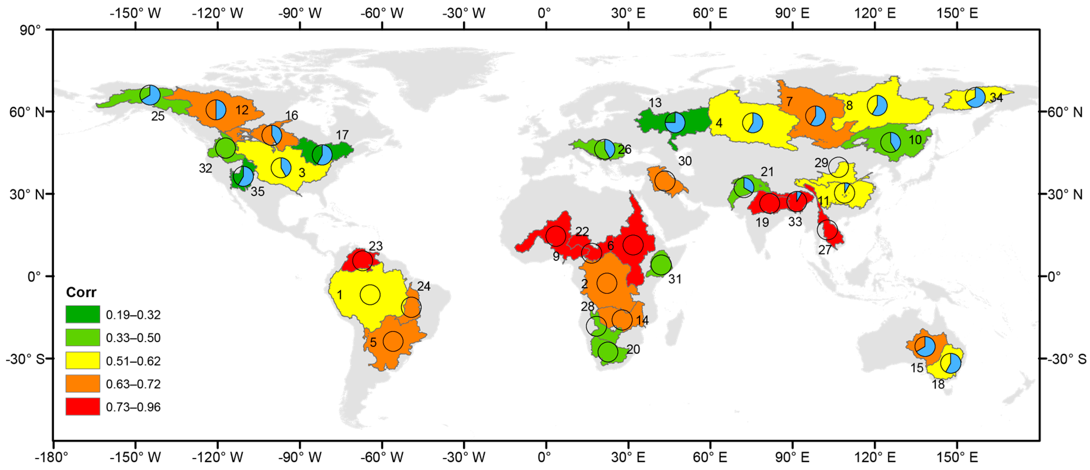
Figure 2.
Empirical mode decomposition (EMD) analysis of Amazon River basin TWSA. Top panel shows the raw data and bottom panel shows the EMD trend. All 5 IMFs are shown in the middle panels. In this case, IMF2 reveals all major TWSA extremes occurred at the basin during the study period.
Figure 2.
Empirical mode decomposition (EMD) analysis of Amazon River basin TWSA. Top panel shows the raw data and bottom panel shows the EMD trend. All 5 IMFs are shown in the middle panels. In this case, IMF2 reveals all major TWSA extremes occurred at the basin during the study period.

Figure 3.
Comparison between TWSA (solid line) and the extreme indicator IMF (dashed line) identified for (a) Mississippi, (b) Nile, (c) Zambezi, and (d) Murray-Darling river basins.
Figure 3.
Comparison between TWSA (solid line) and the extreme indicator IMF (dashed line) identified for (a) Mississippi, (b) Nile, (c) Zambezi, and (d) Murray-Darling river basins.
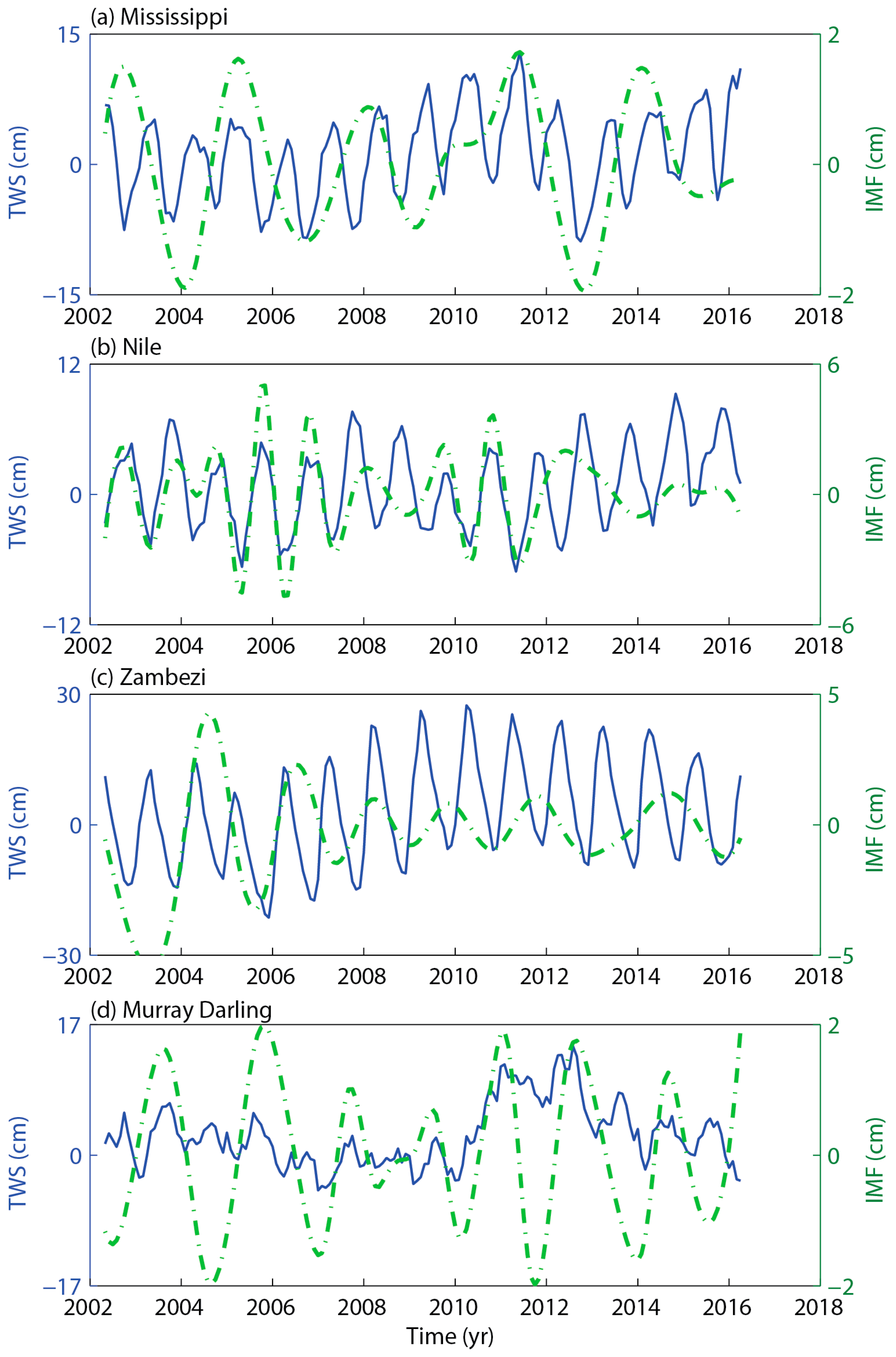
Figure 4.
BPs detected over (a) Amazon, (b) Mississippi, (c) Nile, and (d) Zambezi river basins. Left axis: CSR-M TWSA (dark gray line), BFAST trends (solid green line), breakpoints (vertical dotted line), confidence intervals (light green shades); right axis: SPI (filled gray areas) and ±1 SPI thresholds (horizontal dotted lines).

Figure 5.
Standardized TWSA derived using TWSA climatology for (a) Amazon, (b) Mississippi, (c) Nile, and (d) Zambezi river basins. Left axis: standardized TWSA smoothed using 3-month moving average (dark green line with filled dots); right axis: SPI (filled gray areas) and ±1 thresholds (horizontal dotted lines). TWSA anomalous events were extracted using the ±1 thresholds.
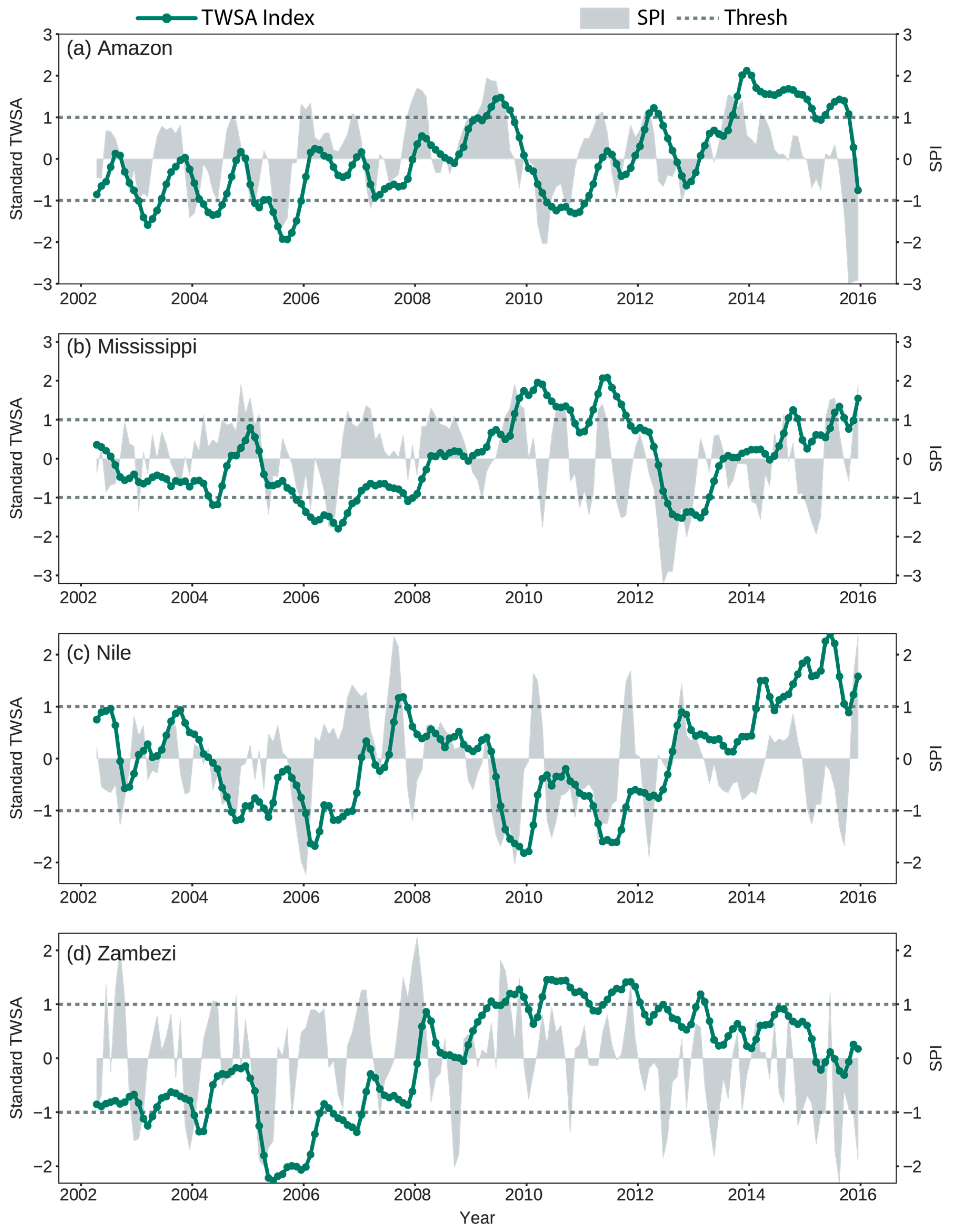
Figure 6.
Heat map of BP coincidence among 35 river basins. The number of BPs for each basin is labeled on the diagonal axis. Each pixel on heat map represents pairwise basin event coincidence rate. Basin pairs having coincidence rate <0.2 are shown as blanks.
Figure 6.
Heat map of BP coincidence among 35 river basins. The number of BPs for each basin is labeled on the diagonal axis. Each pixel on heat map represents pairwise basin event coincidence rate. Basin pairs having coincidence rate <0.2 are shown as blanks.

Figure 7.
Comparison of BPs detected using 3 different GRACE products, CSR-M (blue with open circles), scaled CSR gridded SH (CSR-SF) (brown), and JPL mascon (JPL-M) (green) for (a) Amazon, (b) Mississippi, (c) Nile, and (d) Zambezi river basins. BPs (vertical dashed lines) detected by CSR-M and JPL-M are similar, while those by CSR-SF show noticeable discrepancies.

Figure 8.
Maximum BP (in absolute magnitude) obtained for each grid block in Mississippi River basin.
Figure 8.
Maximum BP (in absolute magnitude) obtained for each grid block in Mississippi River basin.

Table 1.
List of 35 global basins examined in this study. AI represents aridity index, CoinBP and CoinTC represent event coincidence rates calculated using BP and TC methods, respectively, P-TWSA lag is in months. Under the Climate column: H-human, SH-semihumid, SA-semiarid, and A-arid. Irrigation area is given as percentage of basin areas.
| ID | Basin | Area (×103 km2) | AI | Climate | Mean Period (mon) | P-TWSA Corr. | P-TWSA Lag (mon) | Coin-BP | Coin-TC | Irrig. (%) |
|---|---|---|---|---|---|---|---|---|---|---|
| 1 | Amazon | 6234 | 1.25 | H | 28 | 0.59 | 0 | 1 | 0.80 | 0.15 |
| 2 | Congo | 3759 | 0.89 | H | 24 | 0.65 | 0 | 0.86 | 0.61 | 0.01 |
| 3 | Mississippi | 3253 | 0.68 | H | 24 | 0.62 | −5 | 1 | 0.93 | 3.92 |
| 4 | Ob | 2997 | 0.76 | H | 33.6 | 0.53 | −7 | 1 | 1.00 | 0.23 |
| 5 | Parana | 2988 | 0.76 | H | 24 | 0.69 | 0 | 1 | 1.00 | 0.87 |
| 6 | Nile | 2978 | 0.34 | SA | 15.2 | 0.81 | 0 | 0.9 | 0.75 | 1.77 |
| 7 | Yenisei | 2609 | 0.88 | H | 21 | 0.72 | −7 | 1 | 1.00 | 0.03 |
| 8 | Lena | 2346 | 0.77 | H | 24 | 0.58 | −7 | 1 | 0.89 | 0 |
| 9 | Niger | 2124 | 0.34 | SA | 24 | 0.95 | 0 | 1 | 0.56 | 0.18 |
| 10 | Amur | 1868 | 0.83 | H | 24 | 0.50 | −5 | 1 | 1.00 | 2.04 |
| 11 | Yangtze | 1831 | 1.01 | H | 24 | 0.55 | −1 | NA | 0.88 | 8.4 |
| 12 | MacKenzie | 1740 | 0.76 | H | 42 | 0.66 | −6 | 1 | 0.87 | 0 |
| 13 | Volga | 1407 | 0.89 | H | 24 | 0.32 | −9 | 1 | 0.92 | 0.5 |
| 14 | Zambezi | 1341 | 0.55 | SH | 21 | 0.67 | 0 | 1 | 0.80 | 0.3 |
| 15 | Lake Eyre | 1248 | 0.13 | A | 18.7 | 0.66 | −8 | 1 | 0.63 | 0 |
| 16 | Nelson | 1110 | 0.67 | H | 21 | 0.65 | −5 | 1 | 0.92 | 0.6 |
| 17 | St. Lawrence | 1109 | 1.1 | H | 33.6 | 0.25 | −7 | 1 | 0.55 | 0.48 |
| 18 | Murray Darling | 1070 | 0.36 | SA | 24 | 0.60 | −7 | 1 | 0.90 | 2.46 |
| 19 | Ganges | 1032 | 0.73 | H | 28 | 0.89 | 0 | 1 | 0.84 | 30.62 |
| 20 | Orange | 999 | 0.22 | SA | 28 | 0.42 | 0 | 1 | 0.90 | 0.63 |
| 21 | Indus | 971 | 0.39 | SA | 24 | 0.41 | −4 | 1 | 0.65 | 22.71 |
| 22 | Chari | 925 | 0.4 | SA | 21 | 0.96 | 0 | 1 | 0.72 | 0.13 |
| 23 | Orinoco | 912 | 1.34 | H | 21 | 0.83 | 0 | 1 | 1.00 | 0.94 |
| 24 | Tocantins | 876 | 0.99 | H | 24 | 0.69 | 0 | 1 | 1.00 | 0.21 |
| 25 | Yukon | 851 | 0.69 | H | 28 | 0.50 | −8 | 1 | 0.52 | 0 |
| 26 | Danube | 806 | 0.91 | H | 33.6 | 0.41 | −5 | 1 | 1.00 | 4.78 |
| 27 | Mekong | 804 | 0.99 | H | 24 | 0.88 | 0 | 1 | 0.93 | 3.77 |
| 28 | Okavango | 793 | 0.29 | SA | 33.6 | 0.50 | 0 | 1 | 0.76 | 0.02 |
| 29 | Yellow | 786 | 0.52 | SH | 21 | 0.57 | 0 | 1 | 0.67 | 9.19 |
| 30 | Euphrates | 762 | 0.27 | SA | 21 | 0.67 | 0 | 1 | 0.97 | 10.15 |
| 31 | Juba | 741 | 0.26 | SA | 15.3 | 0.43 | 0 | 1 | 0.84 | 0.17 |
| 32 | Columbia | 722 | 0.78 | H | 33.6 | 0.45 | 0 | 1 | 0.67 | 3.98 |
| 33 | Bramaputra | 657 | 1.19 | H | 28 | 0.79 | −1 | 1 | 0.92 | 6.55 |
| 34 | Kolyma | 640 | 0.75 | H | 28 | 0.56 | −8 | 1 | 0.96 | 0 |
| 35 | Colorado | 636 | 0.27 | SA | 24 | 0.19 | −7 | 1 | 0.58 | 2.27 |
© 2017 by the authors. Licensee MDPI, Basel, Switzerland. This article is an open access article distributed under the terms and conditions of the Creative Commons Attribution (CC BY) license (http://creativecommons.org/licenses/by/4.0/).
Share and Cite
MDPI and ACS Style
Sun, A.Y.; Scanlon, B.R.; AghaKouchak, A.; Zhang, Z. Using GRACE Satellite Gravimetry for Assessing Large-Scale Hydrologic Extremes. Remote Sens. 2017, 9, 1287. https://doi.org/10.3390/rs9121287
AMA Style
Sun AY, Scanlon BR, AghaKouchak A, Zhang Z. Using GRACE Satellite Gravimetry for Assessing Large-Scale Hydrologic Extremes. Remote Sensing. 2017; 9(12):1287. https://doi.org/10.3390/rs9121287
Chicago/Turabian StyleSun, Alexander Y., Bridget R. Scanlon, Amir AghaKouchak, and Zizhan Zhang. 2017. "Using GRACE Satellite Gravimetry for Assessing Large-Scale Hydrologic Extremes" Remote Sensing 9, no. 12: 1287. https://doi.org/10.3390/rs9121287
Note that from the first issue of 2016, this journal uses article numbers instead of page numbers. See further details here.