
S-Band Doppler Wave Radar System


1
School of Electronic Information and the Collaborative Innovation Center for Geospatial Technology, Wuhan University, Wuhan 430072, China
2
School of Electronic Information, Wuhan University, Wuhan 430072, China
*
Author to whom correspondence should be addressed.
Remote Sens. 2017, 9(12), 1302; https://doi.org/10.3390/rs9121302
Submission received: 27 October 2017
/
Revised: 8 December 2017
/
Accepted: 11 December 2017
/
Published: 12 December 2017
(This article belongs to the Special Issue Instruments and Methods for Ocean Observation and Monitoring)
Abstract
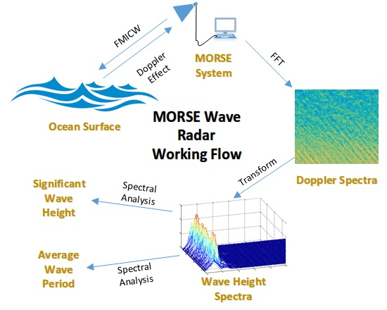
:In this paper, a novel shore-based S-band microwave Doppler coherent wave radar (Microwave Ocean Remote SEnsor (MORSE)) is designed to improve wave measurements. Marine radars, which operate in the X band, have been widely used for ocean monitoring because of their low cost, small size and flexibility. However, because of the non-coherent measurements and strong absorption of X-band radio waves by rain, these radar systems suffer considerable performance loss in moist weather. Furthermore, frequent calibrations to modify the modulation transfer function are required. To overcome these shortcomings, MORSE, which operates in the S band, was developed by Wuhan University. Because of the coherent measurements of this sensor, it is able to measure the radial velocity of water particles via the Doppler effect. Then the relation between the velocity spectrum and wave height spectrum can be used to obtain the wave height spectra. Finally, wave parameters are estimated from the wave height spectra by the spectrum moment method. Comparisons between MORSE and Waverider MKIII are conducted in this study, and the results, including the non-directional wave height spectra, significant wave height and average wave period, are calculated and displayed. The correlation coefficient of the significant wave height is larger than 0.9, whereas that of the average wave period is approximately 0.4, demonstrating the effectiveness of MORSE for the continuous monitoring of ocean areas with high accuracy.

1. Introduction
The non-coherent and coherent method are the two main methods used in radio ocean remote sensing. The non-coherent method utilizes a non-coherent radar to acquire the backscatter images of the targeted ocean area. Then 3D-FFT(three dimensional fast fourier transformation) is applied to the acquired images to obtian the spectra. Finally, the ocean dynamic parameters are deduced by a spectral analysis of the spectra [1]. The radar used in this method can be modified from a marine navigation radar, which makes it a low-cost and flexible method of monitoring oceans. However, the modulation transfer function is always needed during the calibration of the results [2]. In the shallow water area, factors such as offshore winds could significantly influence the results [3]. The coherent method employs a Doppler coherent radar to measure the radial wave velocity [4], and the wave height spectra are derived via a certain relation between the radial velocity and the wave height spectrum. Eventually the ocean dynamic parameters are extracted from the wave height spectra [5]. Compared with the non-coherent method, the coherent method does not require calibration, and is adaptive in various bathymetry areas; therefore, the coherent method is promising for monitoring oceans with radars and worth further research.
In 1985, Young et al. extracted the wave and current parameters from the echoes of an X-band marine radar [1]. Since then, the non-coherent method utilizing X-band radar has been well investigated. Multiple algorithms, such as the basic LS (Least Square) fitting method [1], weighted LS method [6], ILS (Iterative LS) approach [7], DiSC (dispersive surface classificatory) method [8], the Polar Current Shell algorithm [9], the Normalized Scalar Product method [10], have been examined by researchers to improve the non-coherent method. Research and measurements of the modulation transfer function have been completed [11,12,13]. Various mature systems, such as WaMos II, which was developed by OceanWaves GmbH in Germany, and WAVEX, which was developed by MIROS in Norway, have also been implemented. However, a precise modulation transfer function, which is difficult to obtain, is the decisive accuracy factor. The study of the coherent method began in the 1980s when Plant and Schuler proposed a preliminary theory and approach for deducing wave height spectra from the velocity of water particles [14,15]. In the 1990s, various experiments using microwave Doppler radar were conducted [5,16,17,18,19]; however, none of the experimental results fully obtained the directional wave height spectra. Recently, the coherent method has been applied on the X-band radar, and the results are very good [20]. SM050, which was developed by MIROS in Norway, is the only mature Doppler marine radar system and it functions in C band and is capable of outputting accurate results one range cell at a time.
To achieve the coherent method, the use of MORSE (Microwave Ocean Remote SEnsor), a shore-based microwave Doppler marine radar system developed by Wuhan University, is proposed. The six antennas equipped with MORSE have a beam width of 30 degrees, which enables MORSE to obtain the full wave height spectrum. MORSE has been deployed in Zhujiajian, Zhejiang and Shanwei, Guangdong Province and it has successfully acquired the wave parameters of targeted ocean areas. In Section 2, we provide a brief description of the coherent wave measuring method. In Section 3, the MORSE system is introduced. In Section 4, a comparison between MORSE and a Waverider MKIII buoy is performed showed and discussed. Finally, in Section 5, the conclusions of the paper are presented.
2. Coherent Wave Measuring Method
According to the Bragg scattering theory and the composite surface scattering theory, backscattering occurs when electromagnetic wave grazes onto the sea surface [16,21]. The middle- and large-scale waves on the sea surface cause multiple modulations of capillary waves. Those modulations make the central frequency of the echoes shift and the bandwidth extend [22,23,24,25], and the wave parameters can be deduced from the reflection of these influences in the echoes.
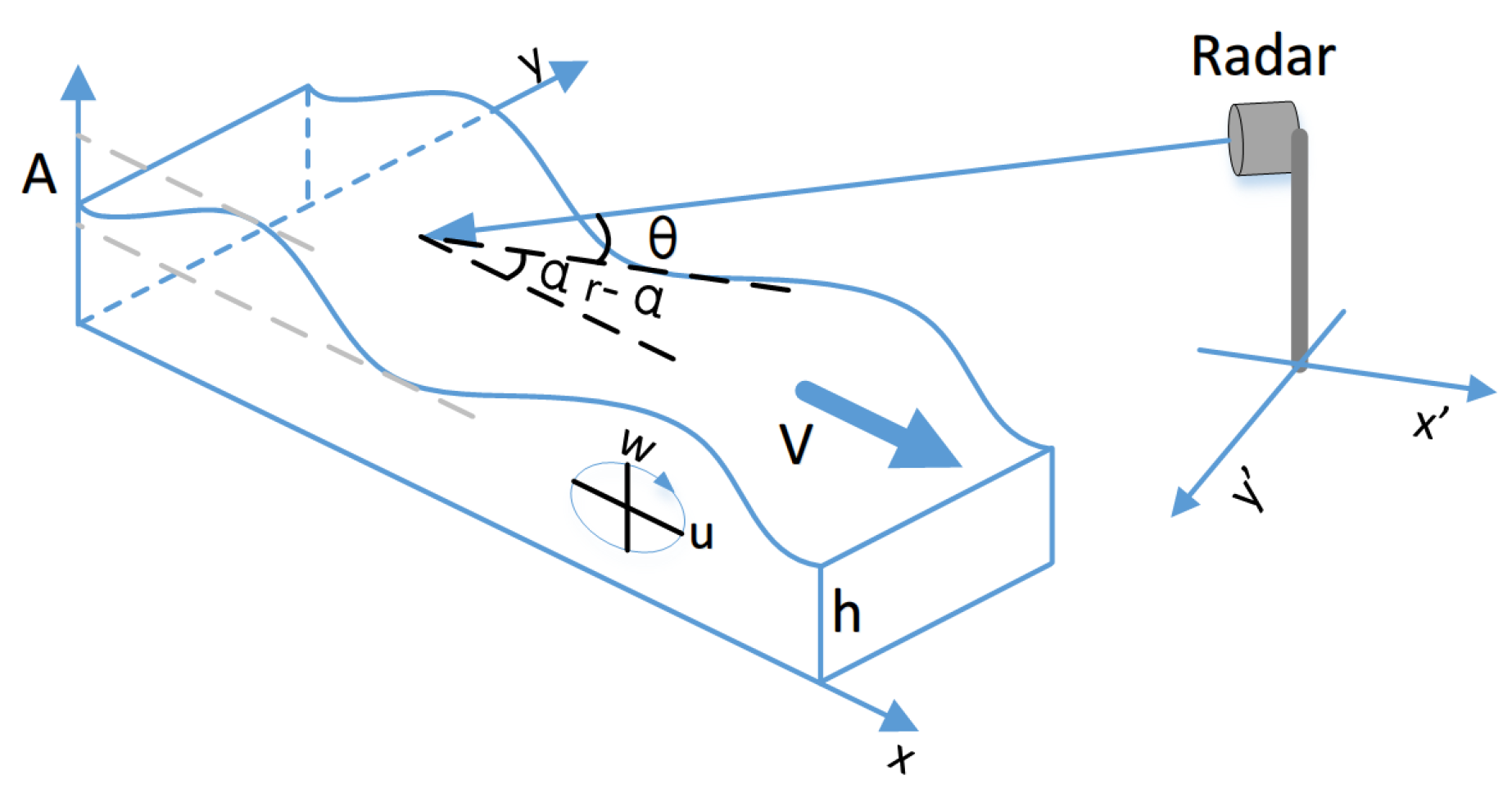
The radial velocity measured by Doppler radar is the sum of the scattered intrinsic velocity and any surface current component [5]. The expression for the radial velocity at a point, under the action of a single long ocean wave with amplitude, angular frequency, wavenumber A(f), , and K (radial and transverse components and ) respectively, is:
where u and w are the horizontal and vertical components of the orbital velocity, respectively; is the orbital velocity; is the radar grazing angle; is the wave azimuth(tan); is the radar azimuth; is the surface current velocity; is the effective scatterer velocity; R is the distance between radar and the observed ocean area; represents the axis that is vertical to R; V is the long-wave phase velocity; and h is the water depth. The illustration of those symbols is shown in Figure 1.
The velocity spectrum G(,,) is obtained by applying the Fourier transformation to . Then, the relation between the velocity spectrum and wave height spectrum is used to deduce the wave height spectrum E() as follows:
where is the relation between the velocity spectrum and wave height spectrum [5,26]:
where is the normalized spreading function.
The phases from two adjacent range cells acquired simultaneously are compared to solve the 180-degree ambiguity [27].
Assuming that the power density spectra of the velocity sequence of two adjacent range cells acquired with the same antenna are and and is farther from the radar, then the cross spectrum of and is as follows:
where is the complex conjugate of .
A relation is observed between and because of the adjacency of the two range cells:
where k is the wavenumber and the range between two range cells. Either the approaching waves or the receding waves can contribute to the velocity spectrum. Hence, we assume that the expression of the velocity spectrum of the first range cell is as follows:
where and correspond to the approaching waves or the receding waves, respectively. Then, the cross spectrum can be described as follows:
The wave height spectrum corresponding to the coming waves and leaving waves can be solved with the following equations:
is defined as follows:
Finally, the relation between the velocity spectrum and wave height spectrum is rewritten as follows:
After obtaining the directional wave height spectrum, the spectrum moment method and empirical formulas can be applied to obtain the wave parameters, such as the significant wave height and average wave period. The energy distribution of the directional wave height spectrum can also reveal some other wave parameters, such as the main wave direction.
3. MORSE Radar System
The Radio Ocean Remote Sensing Lab of Wuhan University developed the MORSE system. The specifics of the MORSE are in Table 1:
3.1. Radar System Architecture
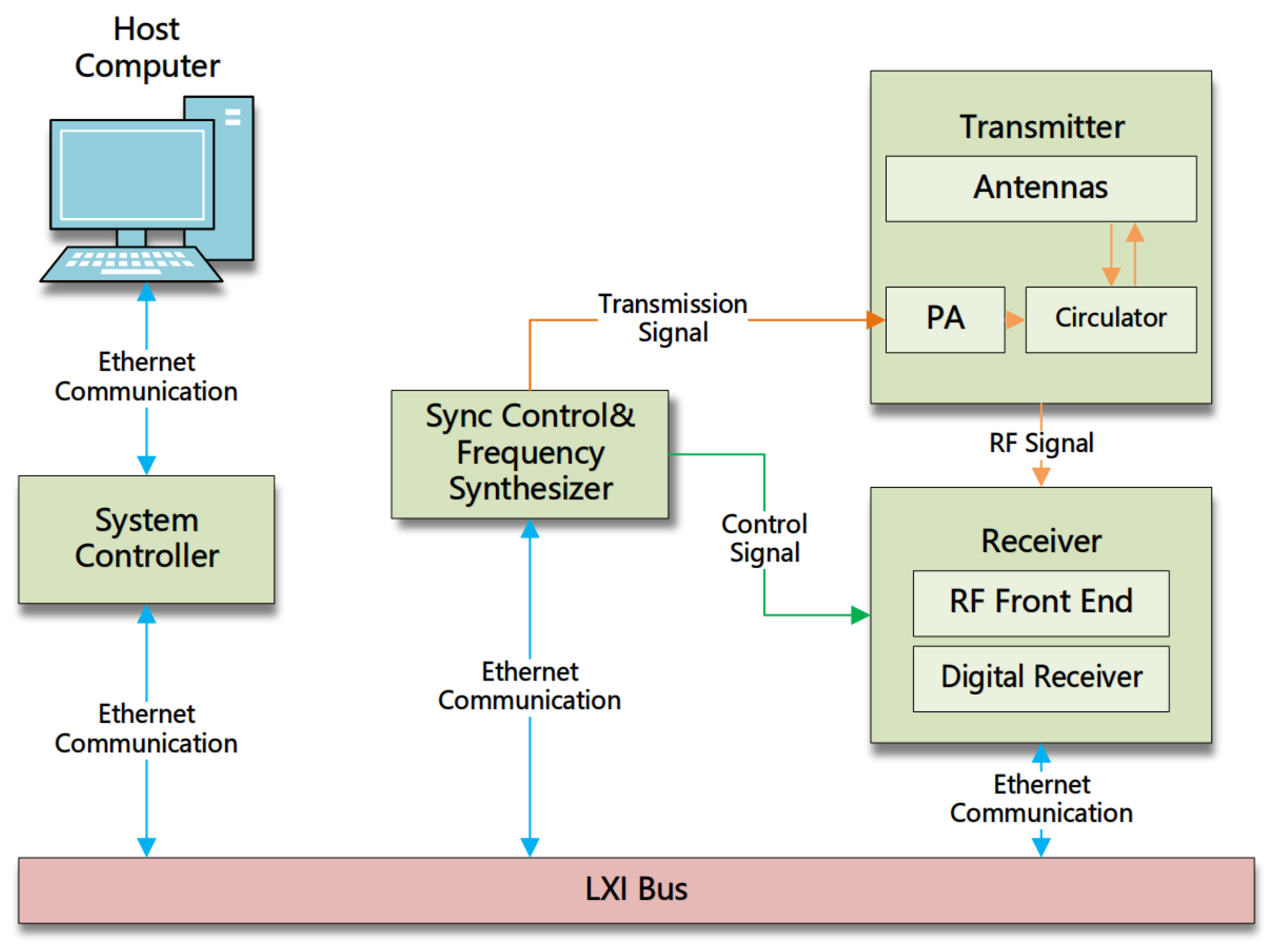
Based on a LXI(LAN eXtensions for Instrumentation) bus, the overall design of MORSE is guided by modularity. All devices involved in MORSE are solid state. The whole system consists of small-scale wideband antennas, high-power switches, power amplifiers, an RF analog front end, a high speed digital receiver, a synchronizing controller, a frequency synthesizer, Ethernet switches and a host computer. The whole system architecture is shown in Figure 2.
The working process of MORSE is as follows. First, after the initialization of the system, the software installed on the computer generates a certain set of waveform parameters based on the radar installation environment and user requirements. Then, the parameters are sent to the synchronizing controller and frequency synthesizer via an Ethernet connection to generate synchronizing and RF signals. The RF signals are sent to the transmitter while the synchronizing signals coordinate the whole system. After the amplification, the RF signals are emitted onto the ocean surface with a low grazing angle by a selected antenna. When the echoes arrive at the radar, they are received by the same antenna and then routed to the RF analog front end for down-conversion. After that, the RF signals are converted into IF signals. Then, the IF signals are sent to digital receivers to generated IQ baseband signals. Finally, these base band signals are fed to the host computer to analyze and deduce the wave parameters.
FMICW (Frequency Modulated Interrupted Continuous Wave) is the waveform that is used by MORSE, and it achieves high range resolution, a long detecting range and the time division multiplexing mode for antennas. The operating frequency of MORSE ranges from 2.75 GHz to 2.95 GHz. A relatively lower operating frequency (compared with X band) deduces the impact caused by the water in the air, which means that MORSE can operate in rainy weather. Because of the pulse compression technique, MORSE uses a small transmitting power of 5 Watts. The frequency sweeping bandwidth is variable among 10 MHz, 20 MHz and 30 MHz, which results in a corresponding range resolution of 15 m, 7.5 m, and 5 m, respectively. The duration of a single frequency sweeping is 4096 s and the interval between two frequency sweeping is 16 s. In addition, a single frequency sweep consists of 128 transmitting pulses with a duty cycle near 50%. Therefore, a Doppler dataset consists of 128 echoes.
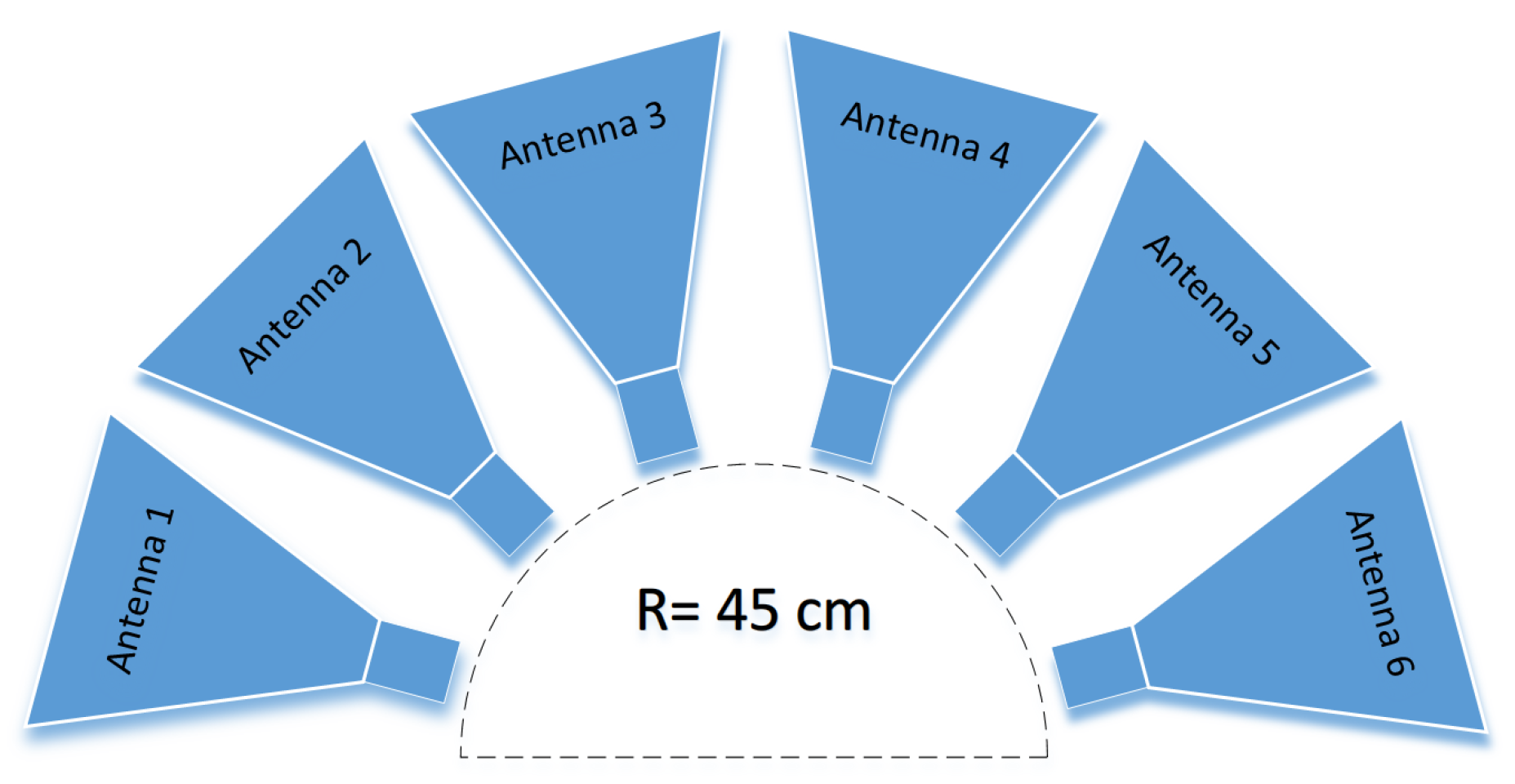
To obtain the full directional wave height spectra, MORSE is equipped with six standard horn-shaped antennas. The shape and placement of antennas are illustrated in Figure 3. These antennas have horizontal and vertical beam widths of 30 degrees and 25 degrees respectively and 15 dB gain. Because the FMICW is adopted by MORSE, these antennas function in time division multiplexing mode. The detecting range could reach 1.5 km with a maximum transmitting power of 5 watts. The antennas cooperate in an electronic scanning mode, and every antenna covers an area of 30 degrees. A single antenna requires 3 min to collecting data; therefore, the total time required for a full directional wave height spectrum is 18 min.
3.2. Algorithm Process
After the down-conversion performed by the RF analog front end and digital receiver, the echoes are transformed into baseband signals. The sample rate of the baseband signals is 125 KHz, and every single baseband signal has 512 sample points.
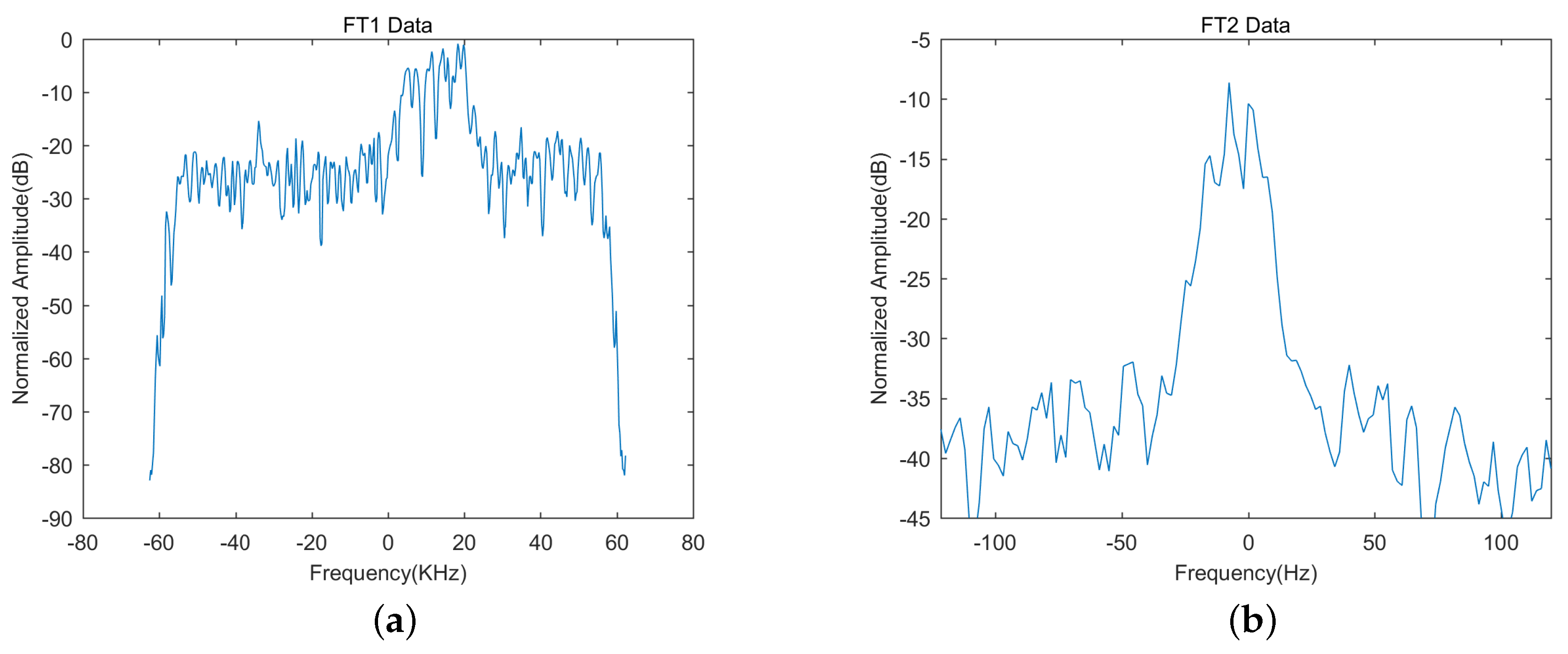
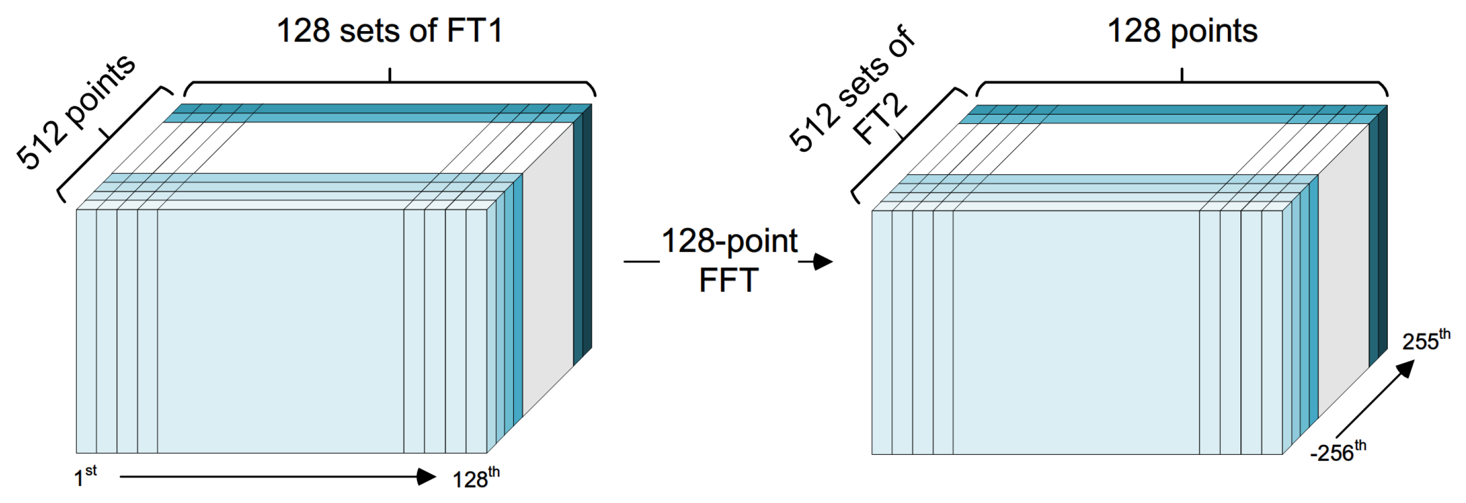
To obtain the Doppler spectra, two FFT will be applied to one Doppler dataset consisting of 128 echoes. After a 512-point FFT applied to every echo, the range spectra, which is named FT1 data, are obtained. The frequency resolution is approximately 244 Hz because the sample rate is 125 KHz. Now we have 128 range spectra and every range spectrum has 512 points. Because every point in a range spectrum represents a range cell. The FT1 data can be viewed from another aspect, which is to say that there are 512 range cells and every range cell has 128 sample points. The sample rate here is the Doppler sample rate. So the Doppler spectra, which is named FT2 data, are then calculated by applying another 128-point FFT to the 128-point data of every range cell. The example of FT1 data and FT2 data is showed in Figure 4. The calculation process of FT2 data is illustrated in Figure 5. The period for the frequency sweep is 4112 s, which means that the sample rate of the Doppler spectra is 243.19 Hz. Hence, the frequency resolution of the Doppler spectra is 1.899 Hz. For one range cell, total time consumption of an 128-point Doppler spectrum sample is 128 × 4112 s ≈ 0.526 s.
The central frequency shift of the Doppler spectra is fundamental to the velocity series. In the MORSE system, the steps to extract central frequency shift are as follows:
- Calculate the peak SNR of a Doppler power density spectrum. First, we take 15 points on the left edge and 15 points on the right edge of a Doppler power density spectrum. Then, we calculate the average of the two sets of points and consider the lower value as the power of noise . Furthermore, we choose the largest value in the spectrum as the maximum signal power . Eventually the SNR is calculated with the following equation:
- Find the bandwidth. We search for 3 points consecutive with the SNR value lower than the threshold (normally 10 dB) from the location of the maximum value to the left and right. Then the locations of the two set of 3 points are treated as the left and right boundaries of the bandwidth are and
- Extract the Doppler frequency shift. We use the spectrum moment method to calculate the frequency shift as follows:
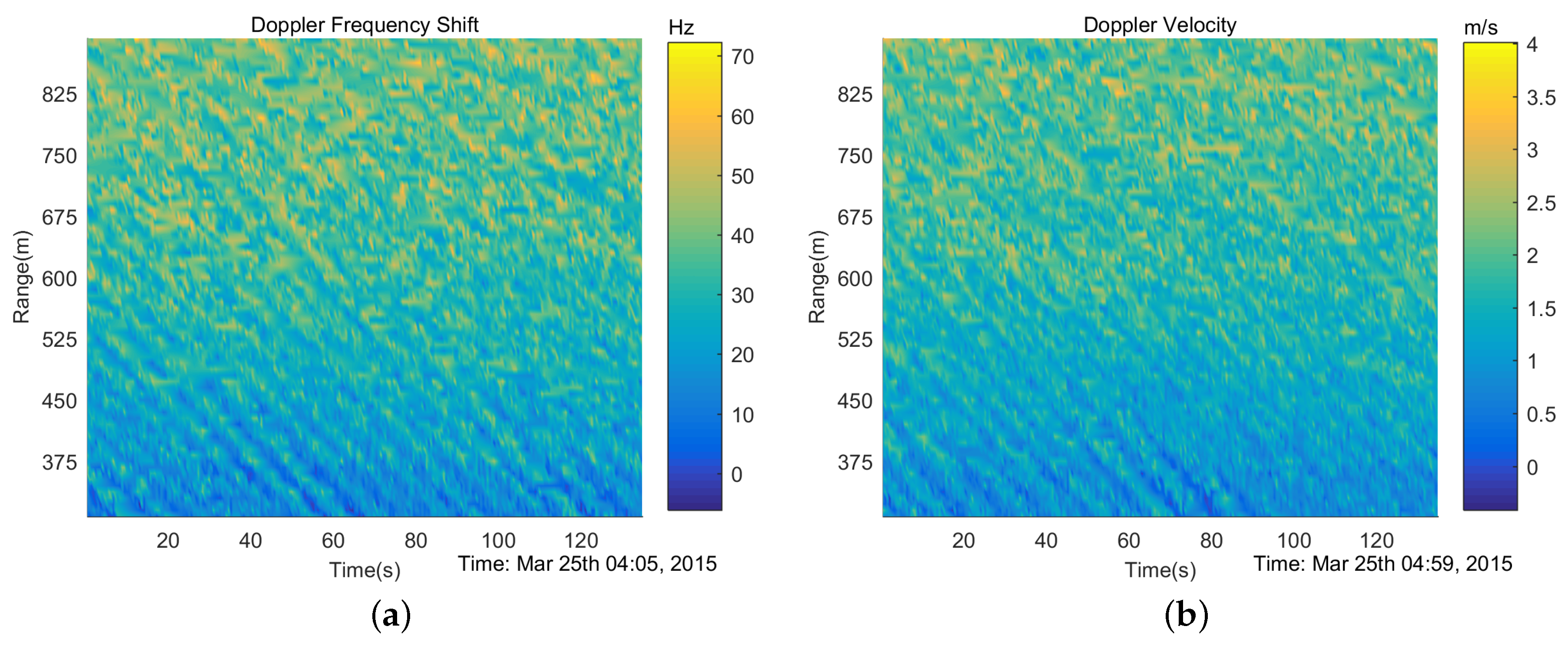
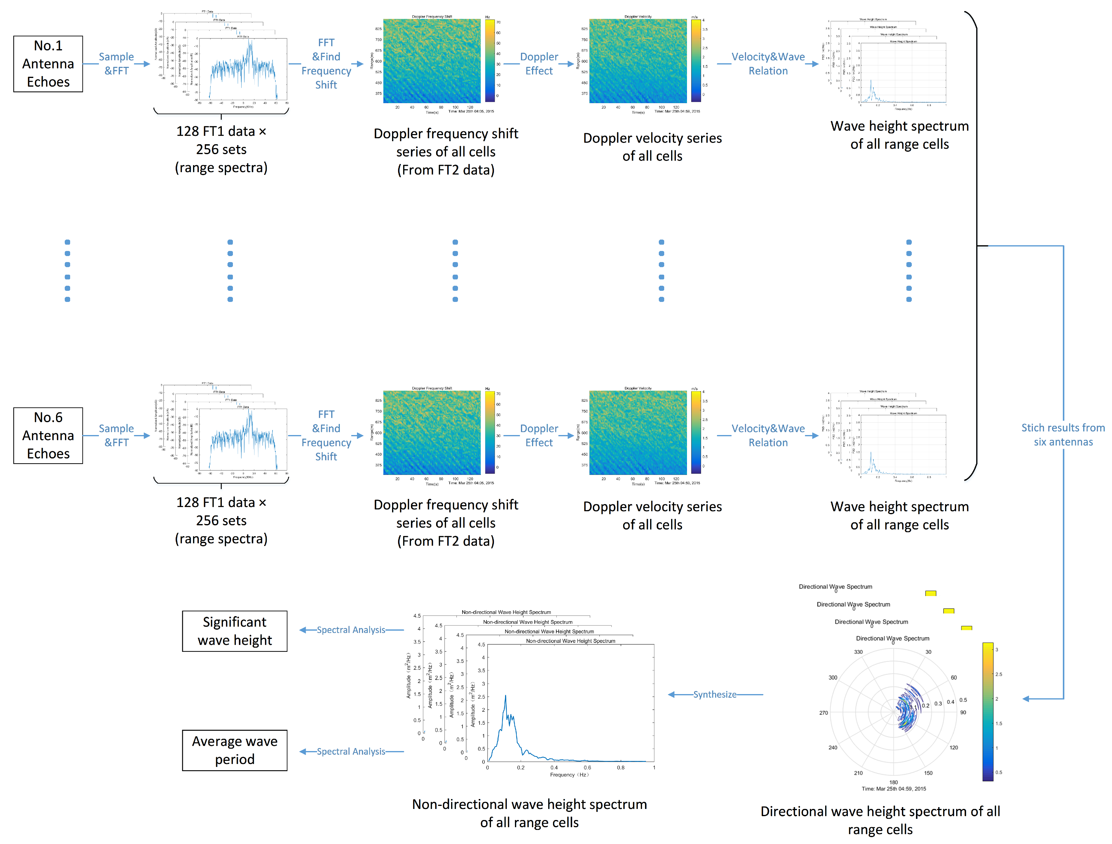
The doppler velocity can then be calculated with the Doppler effect after determining the central Doppler frequency shift of the Doppler spectra. Because the time consumption of an 128-point Doppler spectrum sample is 0.526 s, the doppler velocity of one range cell is calculated every 0.526 s. With each antenna, we calculate 256 doppler velocity to generate one doppler velocity series for every range cell, which takes approximately 134.626 s. The example of Doppler frequency shift spectra and Doppler velocity spectra is showed in Figure 6. Then according to the Formula (6) and (7), the wave height spectrum of that range cell is calculated. In the end, with the spectrum moment method, the wave parameters are obtained using the following equations [28].
First we define the n th order moment :
then (by empirical formula):
Significant wave period :
Peak period , which corresponds to non-directional wave height spectrum peak frequency:
Dominant wave length :
Dominant wave phase velocity :
Average wave period :
The whole data processing approach is demostrated in Figure 7.
4. Results Comparison and Analysis
4.1. Experiment Introduction
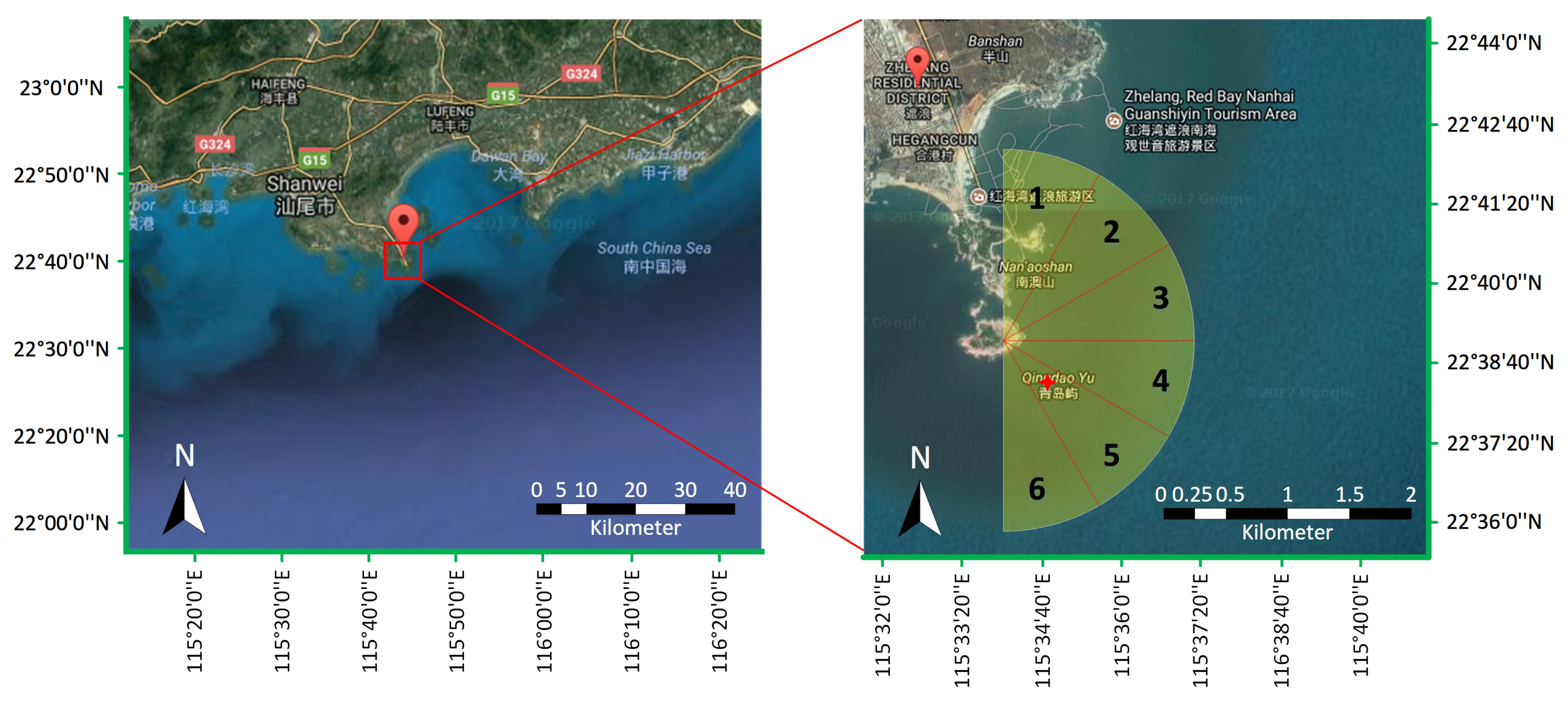
An experiment using MORSE was conducted from 19 March 2015 to 30 March 2015, in Zhelang, Guangdong. The location and the orientation of antennas are demonstrated in Figure 8. A cold front occurred during the experiment, which resulted in strong winds and rain. The wind scale began to increase on March 19 and reached its maximum on approximately March 25. Afterwards, the wind gradually ceased and the temperature rose. Rain fell on March 22 , March 23 and March 26. The azimuth angle covered by antennas is to . The installation position of the antennas is 20 m above the sea level. The No.1 and No.6 antennas were partly sheltered; therefore, the data acquisition rate was low. The data from 18:00 March 23 to 08:00 March 24 were missing because of a power failure caused by exterior reasons.
The radar waveform parameters are listed as follows: operating frequency is 2.85 GHz; frequency sweep period is 4112 s; frequency sweep bandwidth is 20 MHz; number of echo sample points is 512; Doppler sample period is 4112 s, range resolution is 7.5 m. The data processing parameters are listed as follows: number of first FFT(FT1) points is 512; number of second FFT(FT2) points is 128; water depth used in algorithm is 15 m.
A buoy mounting Waverider MKIII was deployed 450 m from the MORSE system. Waverider MKIII is developed by Datewell in Netherlands. The specifics of the Waverider MKIII are as follows: wave height range 0–20 m with a resolution of 0.01 m, wave period 1.6–30 s, wave direction 0–360 with a resolution of . We compared the data of the range cell near the buoy acquired by MORSE with the data acquired by buoy. The buoy generated a dataset every half hour, and these data represented the average of the data in the previous 20 min before the dataset was generated. However, MORSE generated a dataset every 3 min. Hence, we averaged the latter six of ten datasets acquired by MORSE every 30 min to get a similar time resolution with the buoys.
4.2. Directional Wave Height Spectrum
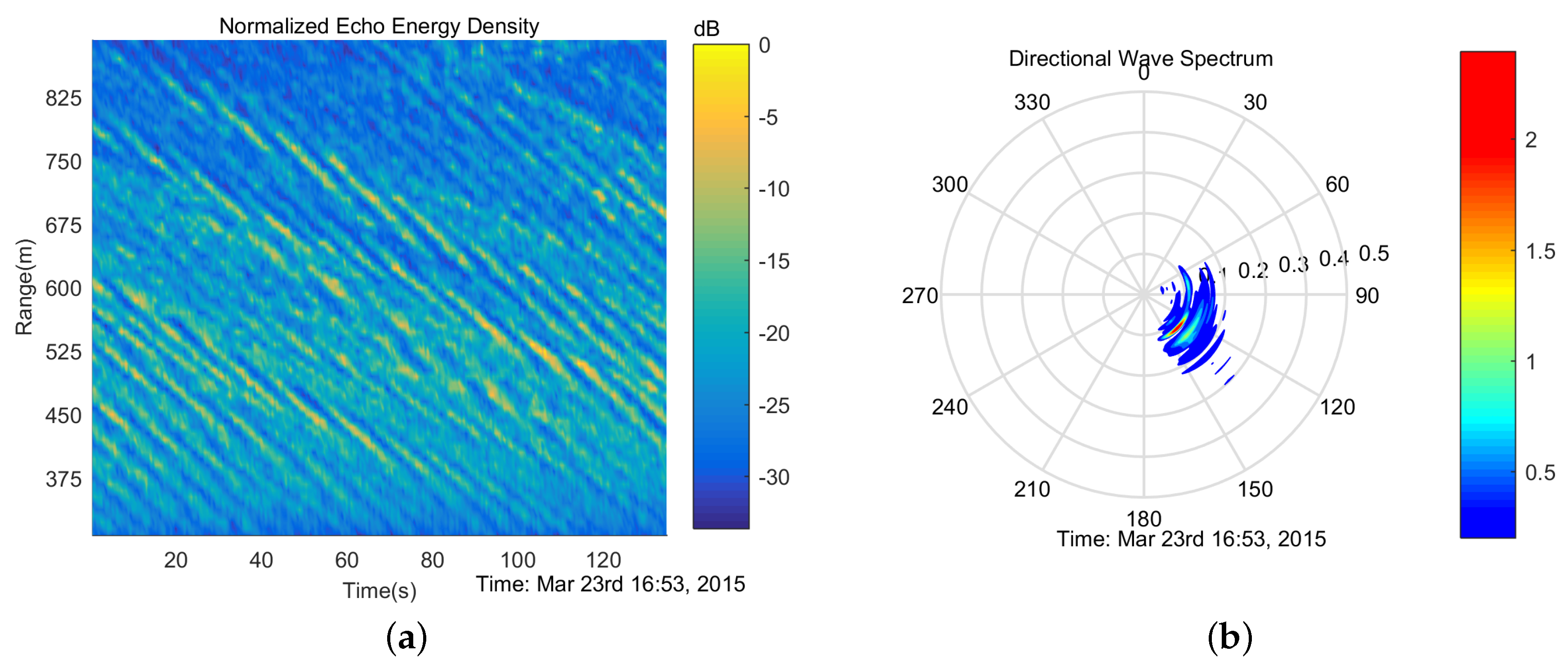
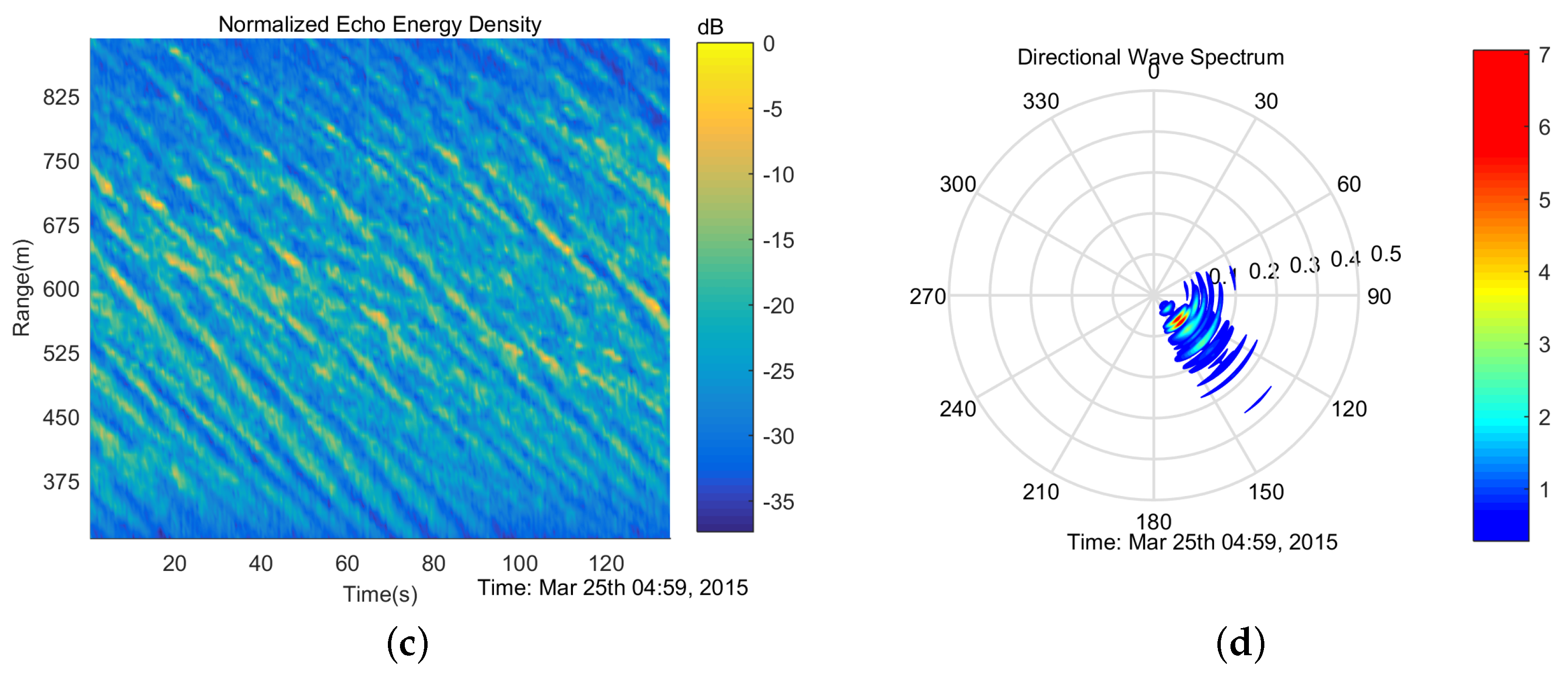
Because the data collection of Waverider MKIII was done by the third party, we did not get the directional wave height spectra data of Waverider MKIII. The Figure 9 below illustrates the normalized echo energy density and the directional wave height spectra. The color bar indicates the intensity. The directional wave height spectrum Figure 9b shows that there are different wave systems at and . Figure 9d only shows one wave system.
4.3. Non-Directional Wave Height Spectrum Comparison
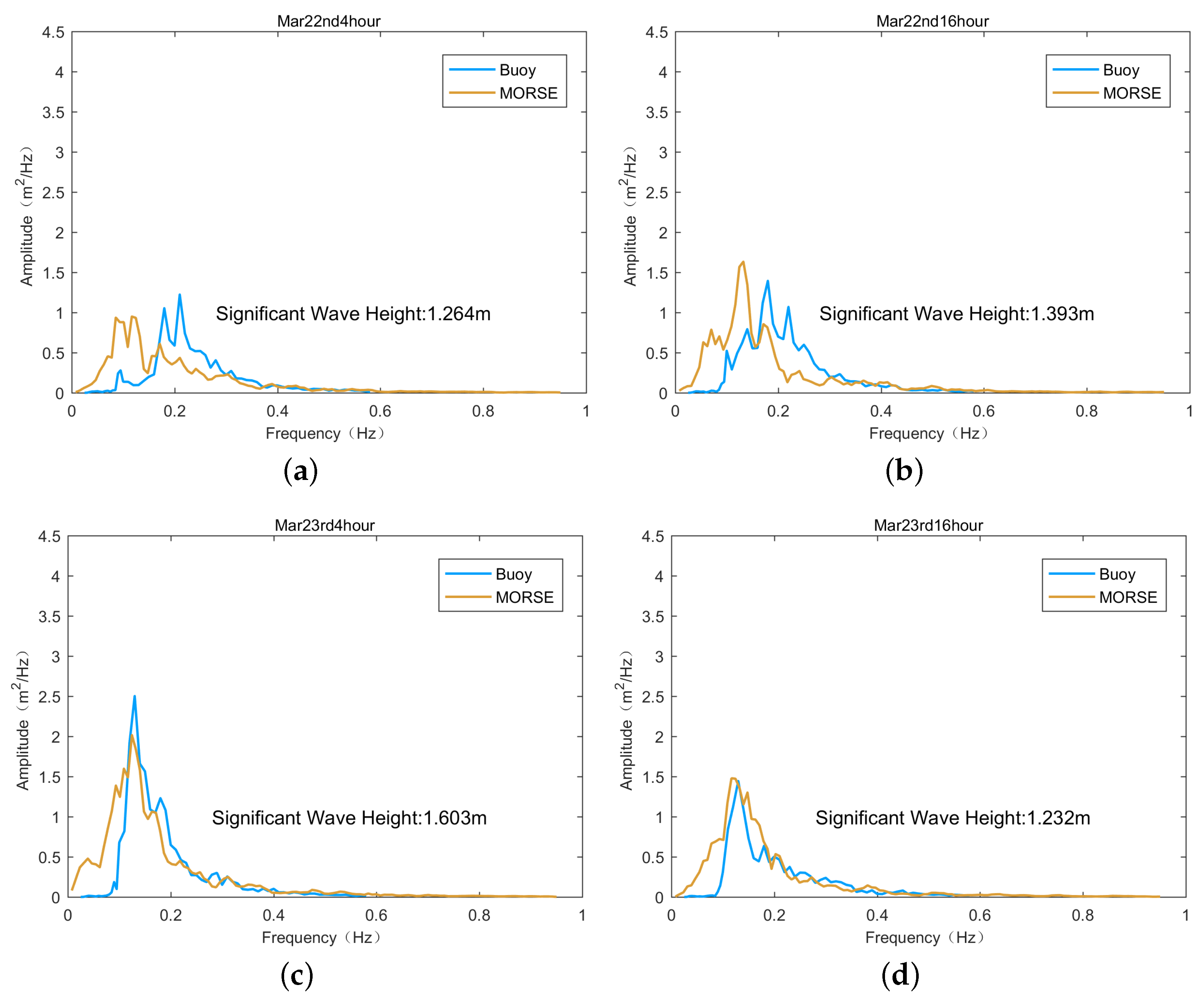
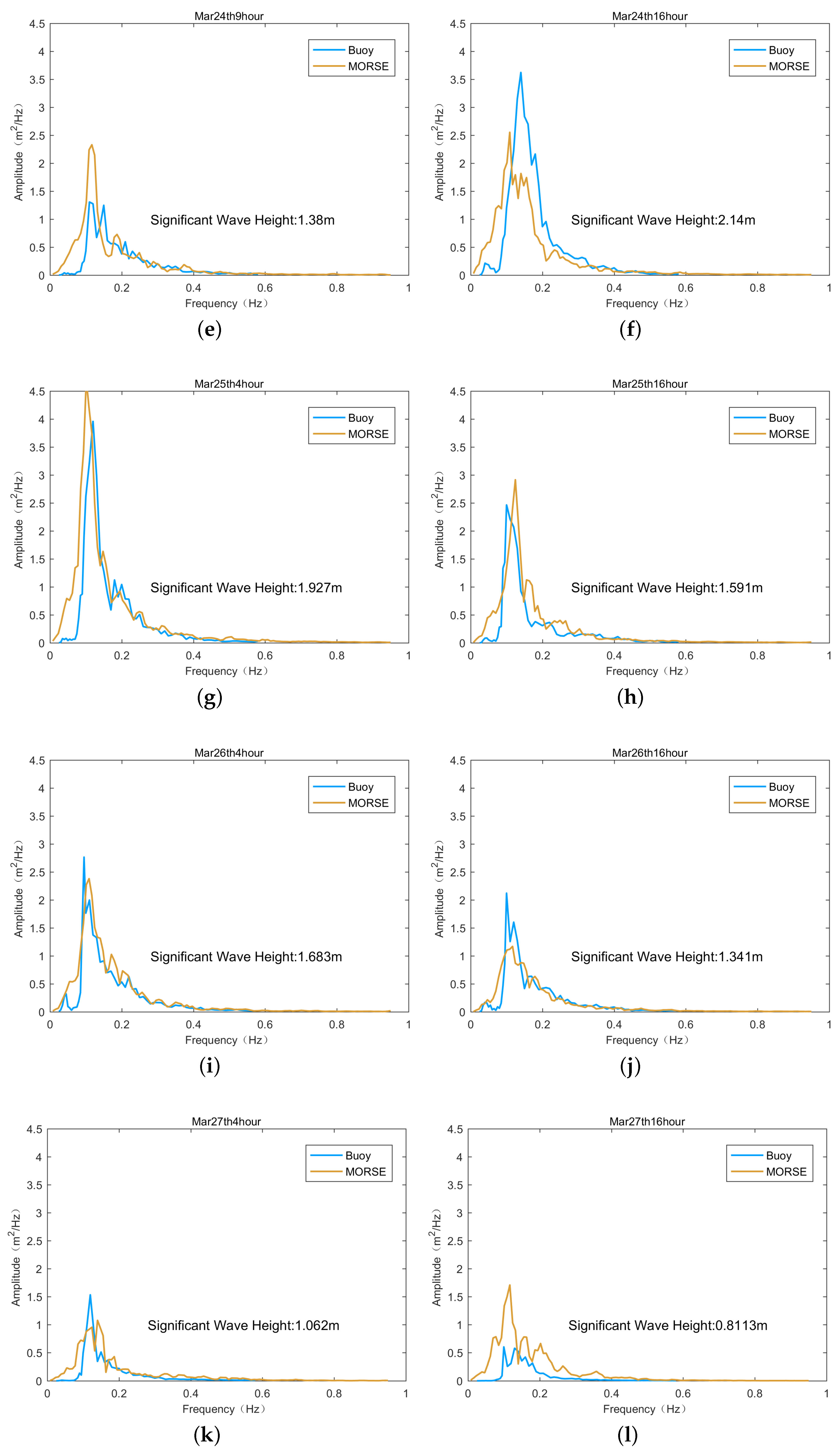
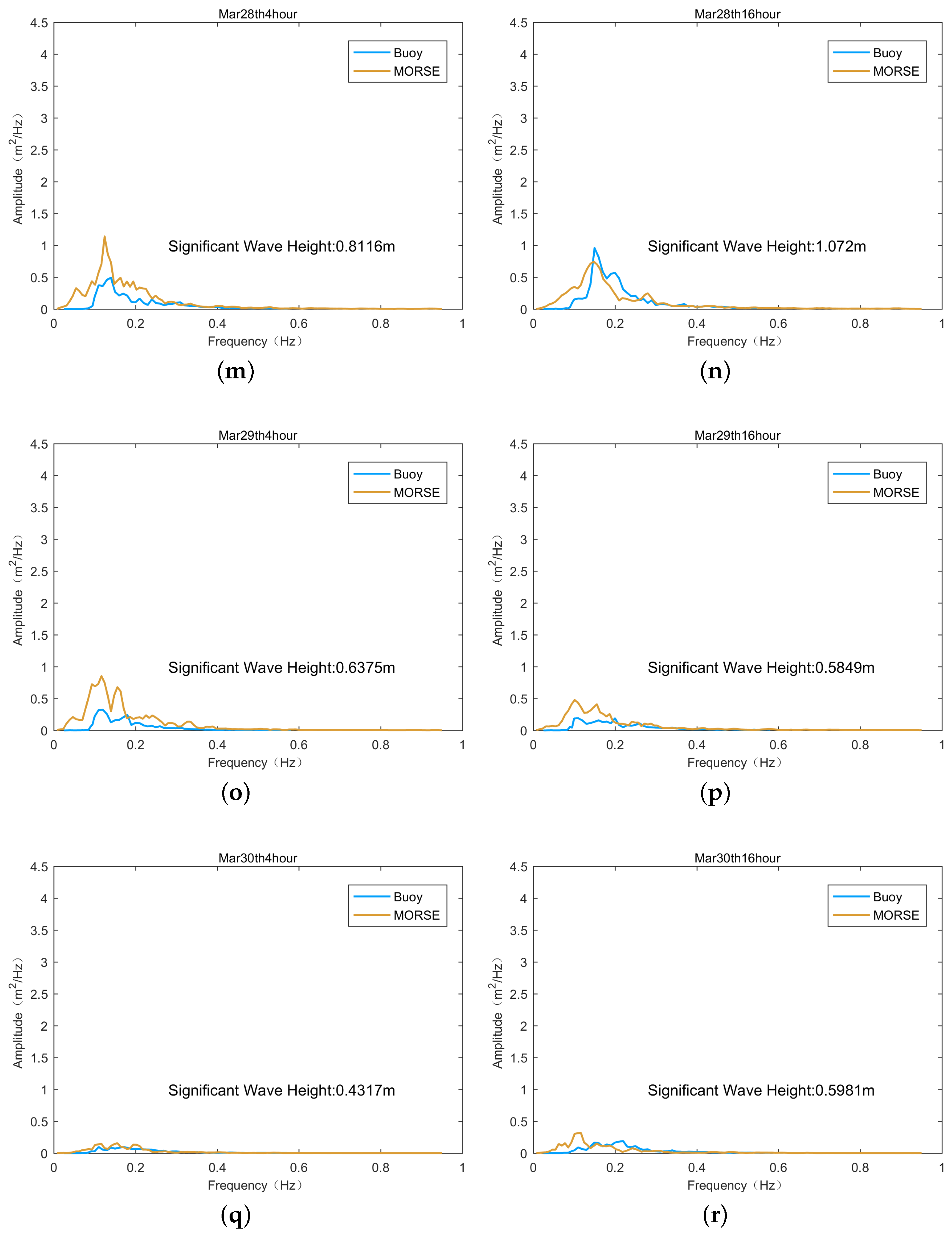
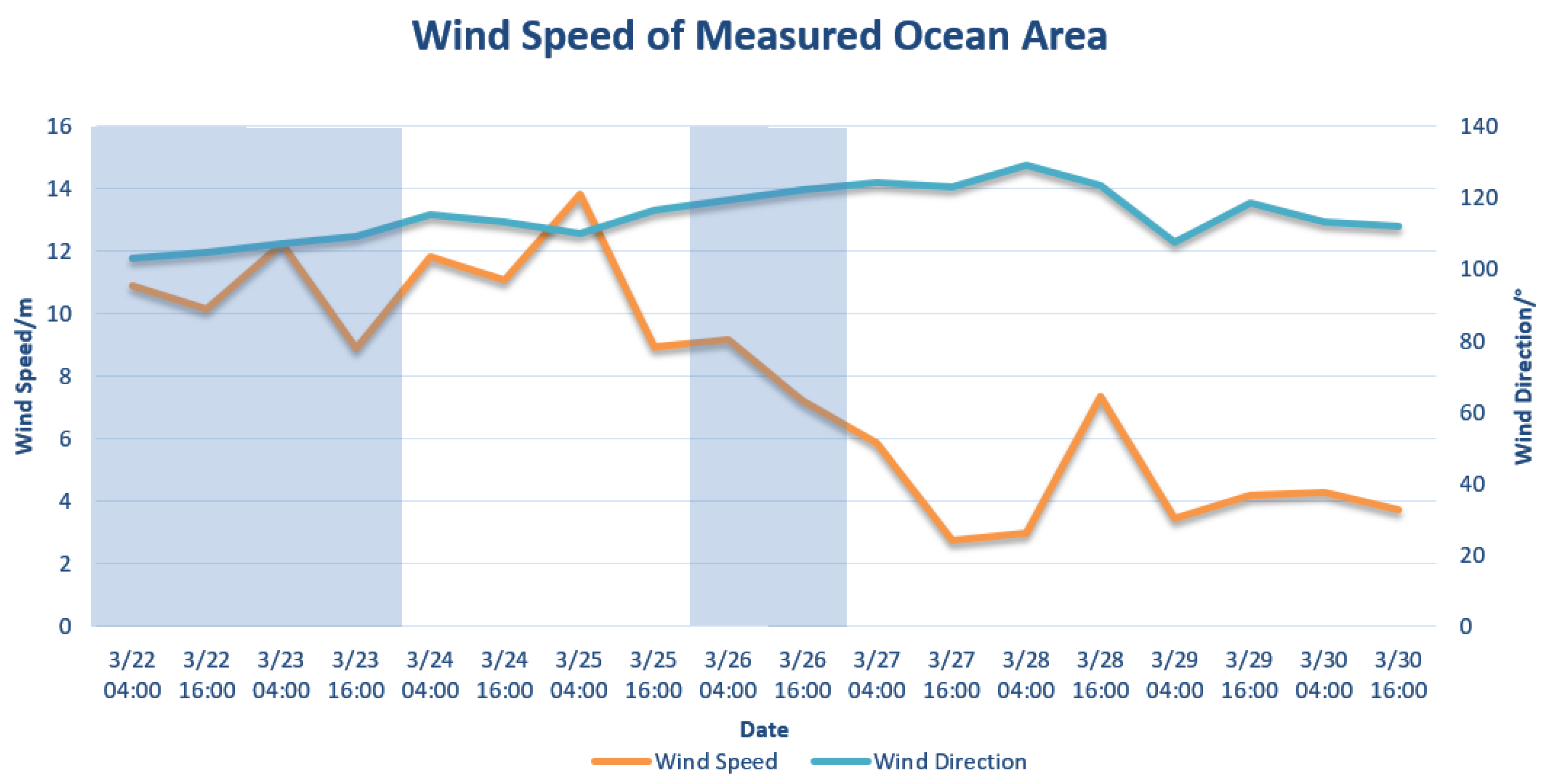
Figure 10 below presents the non-directional wave height spectra measured by both the MORSE system and the buoy. Three-point smoothing was applied on these wave height spectra. The significant wave height measured by the buoy is also illustrated below. Because of a power failure, the data for 04:00 March 24 were missing, and they were replaced by the data of 09:00 March 24. The wind velocity is also plotted in Figure 11.
The spectra indicate that the targeted ocean area was obviously influenced by the cold front. The cold front reached the experimental site on March 22. The wind velocity reached its maximum on March 25 and, then gradually declined. The non-directional wave height spectra illustrate that the wave height started to increase on March 23 and reached its peak on March 25. On March 27, the wave height returned to a lower level. The data derived from the spectra are consistent with the weather conditions.
For comparison, the spectra measured by both instruments are more consistent when the sea state is relatively high. However, when the sea state is low, the sea surface is calm and smooth, which leads to a low SNR of echoes. Hence, the spectra measured by MORSE deviate from those measured by the buoy.
4.4. Significant Wave Height
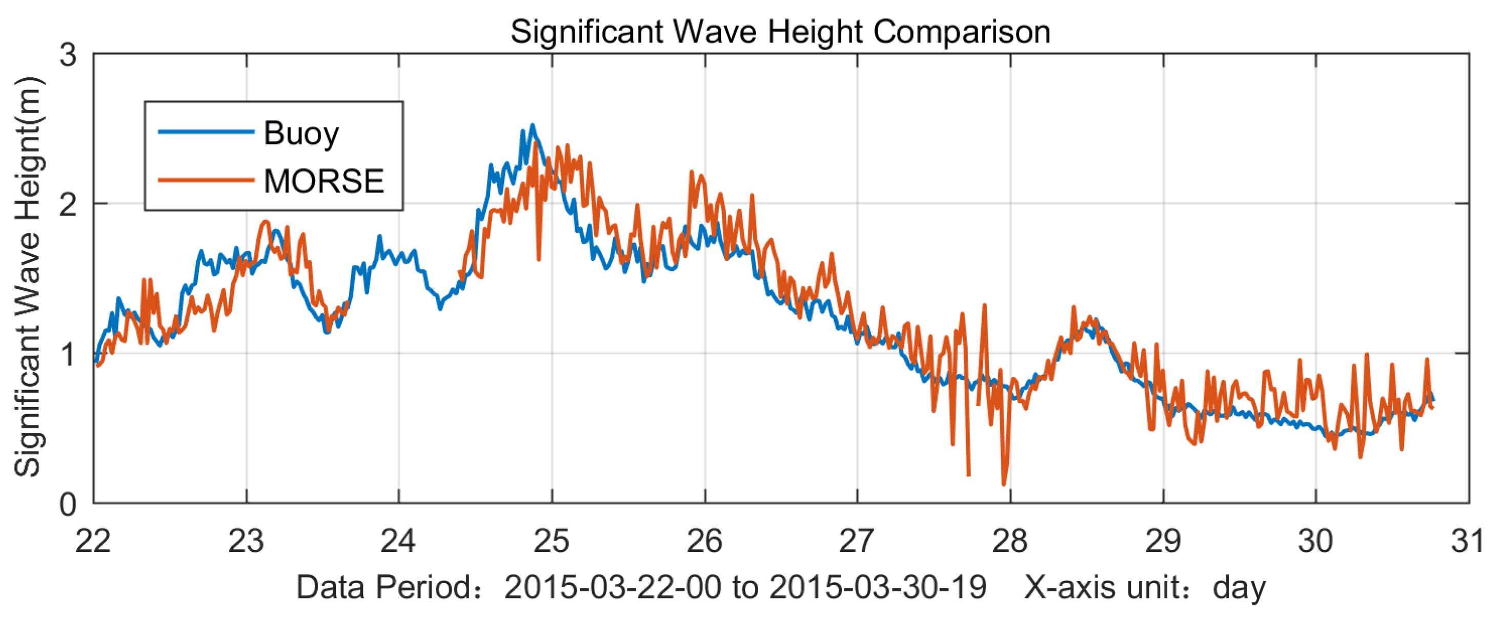
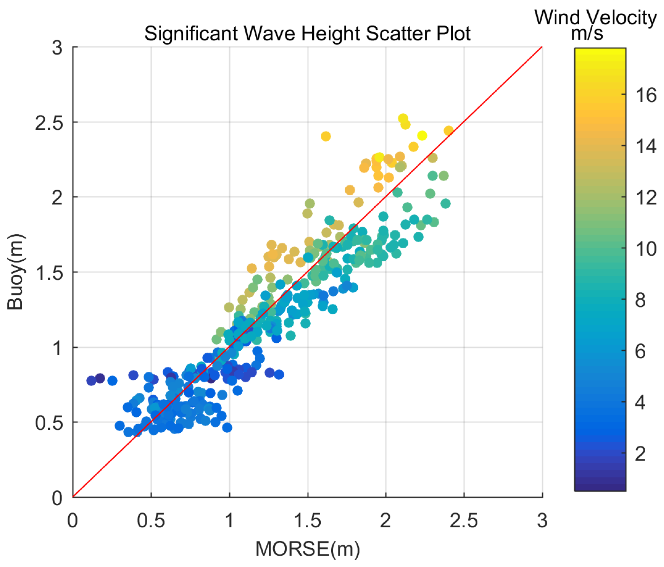
Figure 12 and Figure 13 illustrate a comparison between the significant wave height measured by MORSE and the buoy from 00:00 22 March to 19:00 30 March 2015.
The data points of both instruments are consistent. The correlation coefficient is 0.9238, the mean error is 0.0437 m, the standard deviation error is 0.1979 m, and the root mean square error is 0.2024 m. The scatter plot also shows a tight distribution along the diagonal, which supports the accuracy of the results. It is also shown in the scatter plot that those data points with low wind velocity distribute horizontally, which indicates a less satisfying performance of MORSE under low-wind-velocity condition.
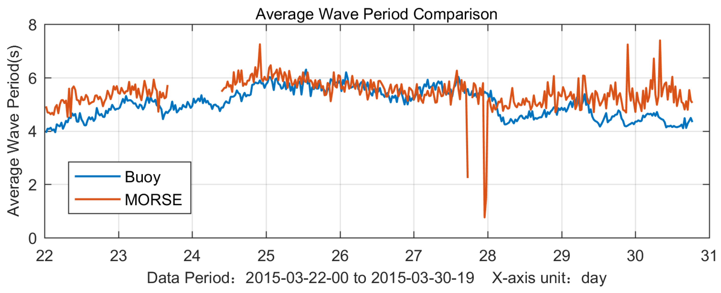
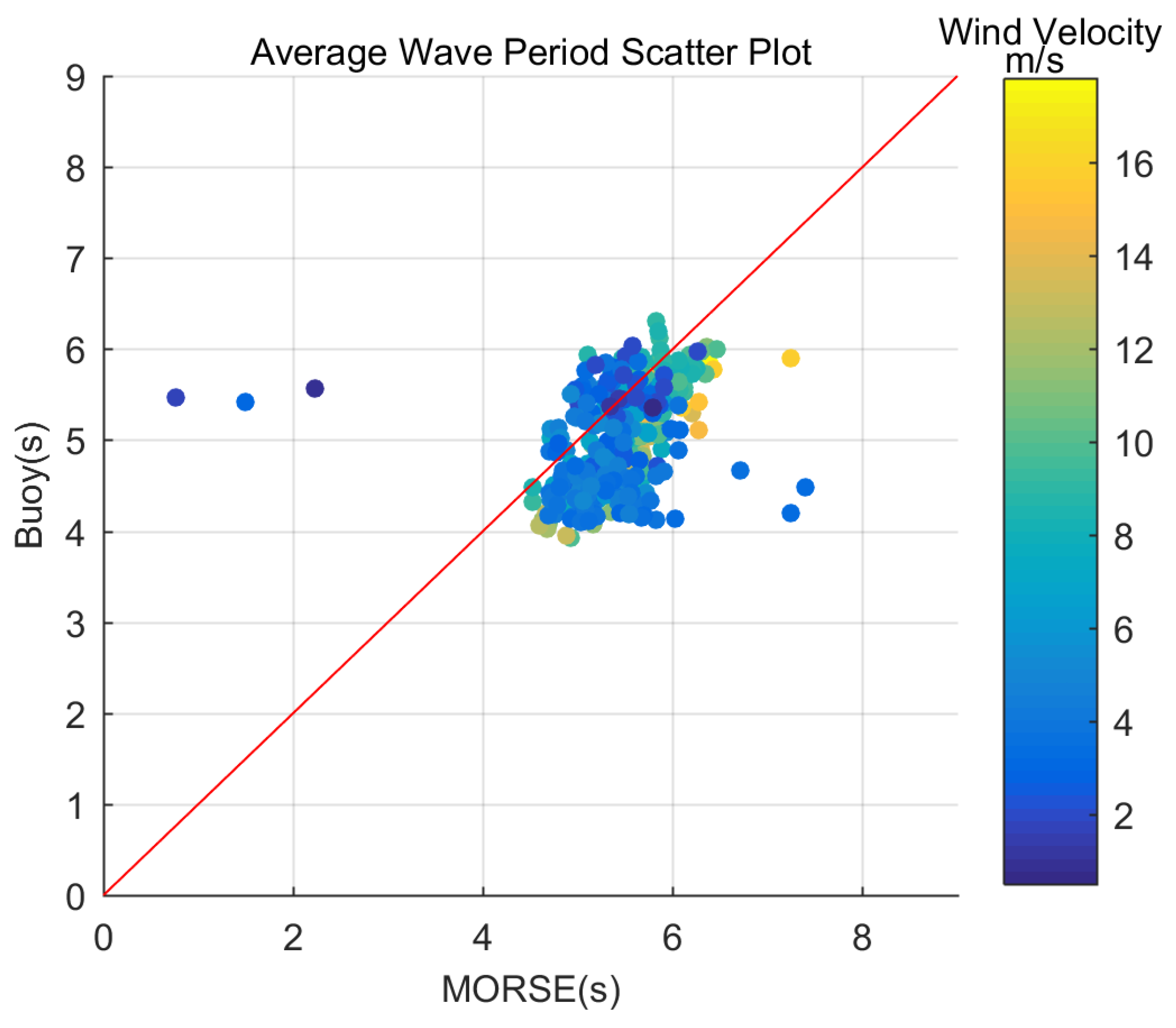
4.5. Average Wave Period
Figure 14 and Figure 15 show a comparison of the average wave period between MORSE and the buoy from 00:00 22 March to 19:00 30 March 2015.
Although the overall trend is similar, the results from MORSE are relatively higher at different levels, especially at the beginning and end of the entire data duration. In addition, certain MORSE data points present much greater deviation from the buoy data during the afternoon and at midnight of March 27. From the scatter plot we can see that those data points with large bias usually have low wind velocity. The average wave period is not as accurate as the significant wave height. The correlation coefficient is 0.3797, the mean error is 0.3938 s, the standard deviation error is 0.6206 s, and the root mean square error is 0.7389 s.
5. Discussion
The comparison of the non-directional wave height spectra shows that the amplitude and shape are consistent, with the spectra correctly showing the change in wave height caused by the cold front. Moreover, during rainy weather, MORSE is still capable of monitoring the ocean and collecting data, which indicates that MORSE is less affected by water in the air. There are good results which prove the ability of MORSE to obtain non-directional wave height spectra. But the non-directional wave height spectra obtained with MORSE show overestimation in low frequency in almost all the examples and frequency shift also appears in some examples such as Figure 10a,b. We have noticed those unsatisfying performance and dug into other data we collected besides that presented in this paper. Unfortunately, we haven’t find the root cause. In the future, we will continue to conduct experiments in different locations and environment. We will also try to get the directional wave height spectra obtained by Waverider MKIII and make a comparison between MORSE and Waverider MKIII.
The accuracy of the significant wave height measured by MORSE, which is shown in the comparison, is good and the trends are consistent. However, when the wave height is low, such as in the afternoon and at midnight on March 27 and from March 29 to March 31, the results fluctuate because of the low SNR of the echoes.
The results of the average wave period comparison are not as satisfying as those of the significant wave height. The MORSE results are approximately 1 s higher when the sea state is low. This bias is also confirmed with the frequency shift in non-directional wave height spectra. After examining the raw MORSE data, we speculate that the cause of the two dips between the afternoon and midnight of March 27, is the ultra-low SNR. The algorithm indicates that few data are valid. The wind velocity corresponding to the two dips is 3 m/s, which could cause SNR deterioration.
Moreover, data processing performed before the comparison could also introduce additional errors. The data period used in analysis is 18 min for MORSE and 20 min for the buoy, are similar but not identical, which could also affect the results. The different data collecting method between MORSE and Waverider MKIII is also a potential factor that contributes to the error. The MORSE switches antenna every 3 min and every antenna’s pointing angle are different. So in other words, the 18-min data collected by MORSE is including all frequency but with one different direction every 3 min. The data collected by Waverider MKIII is including all frequency and all direction. In some case, that may lead to bias.
6. Conclusions
This paper introduces the MORSE system, which is capable of monitoring oceans with the coherent method. By directly measuring the radial velocity of water scatterer, MORSE can obtain the wave height spectra via the relation between the velocity spectrum and wave height spectrum. Then, the ocean dynamic parameters can be derived from the wave height spectra.
Comparisons of the non-directional wave height spectra, significant wave height and average wave period are presented in this paper. The data were acquired in an experiment conducted in March, 2015. Both the amplitude and the shape of the non-directional wave height spectra are consistent with those measured by the buoy. The accuracy of the significant wave height measured by MORSE is validated by a high correlation coefficient of 0.9. However, the results of the average wave period, especially under a low sea state, are not satisfying. Further research will be performed to assess additional factors that could affect the measurement, such as wind. The comparisons presented herein show that MORSE is capable of consistently and accurately monitoring an area of ocean.
Acknowledgments
This work was supported in part by the National Natural Science Foundation of China under Grant No.41376182 and 41506201; in part by National Key Research and Development Plan No.2016YFC1400504 and No.2017YFF0206404; and in part by the Project of Hubei Province Science and Technology Support Program under Grant No.2014BEC057; in part by the Public Science and Technology Research Funds Projects of Ocean under Grant No.201205032.
Author Contributions
Zezong Chen designed the MORSE system. Zihan Wang participated in the module design and development of MORSE and wrote the manuscript. Chen Zhao supervised the preparation of the manuscript and coordinated revisions. Xi Chen, Fei Xie and Chao He participated in the experiment and data processing.
Conflicts of Interest
The authors declare no conflict of interest.
Abbreviations
The following abbreviations are used in this manuscript:
| 3D-FFT | Three dimensional fast fourier transformation |
| FFT | Fast fourier transformation |
| LS | Least square |
| ILS | Iterative least square |
| DiSC | Dispersive surface classificatory |
| MORSE | Microwave ocean remote sensor |
| LXI | LAN extensions for instrumentation |
| FMICW | Frequency modulated interrupted continuous wave |
| SNR | Signal noise ratio |
| RF | Radio frequency |
| IF | Intermediate frequency |
References
- Young, I.R.; Rosenthal, W.; Ziemer, F. A three-dimensional analysis of marine radar images for the determination of ocean wave directionality and surface currents. J. Geophys. Res. 1985, 90, 1049–1059. [Google Scholar] [CrossRef]
- Nieto Borge, J.; RodrÍguez, G.R.; Hessner, K.; González, P.I. Inversion of marine radar images for surface wave analysis. J. Atmos. Ocean. Technol. 2004, 21, 1291–1300. [Google Scholar] [CrossRef]
- Trizna, D.B. Comparisons of a fully coherent and coherent-on-receive marine radar for measurements of wave spectra and surface currents. In Proceedings of the OCEANS 2010, Seattle, WA, USA, 20–23 September 2010. [Google Scholar]
- Dahl, P.H.; Plant, W.J. Simultaneous acoustic and microwave backscattering from the sea surface. J. Acoust. Soc. Am. 1997, 101, 2583–2595. [Google Scholar] [CrossRef]
- Poulter, E.M.; Smith, M.J.; McGregor, J.A. S-Band FMCW Radar Measurements of Ocean Surface Dynamics. J. Atmos. Ocean. Technol. 2008, 10, 142–149. [Google Scholar] [CrossRef]
- Gangeskar, R. Ocean current estimated from X-band radar sea surface, images. IEEE Trans. Geosci. Remote Sens. 2002, 40, 783–792. [Google Scholar] [CrossRef]
- Senet, C.M.; Seemann, J.; Flampouris, S.; Ziemer, F. Determination of bathymetric and current maps by the method DiSC based on the analysis of nautical X-band radar image sequences of the sea surface. IEEE Trans. Geosci. Remote Sens. 2008, 46, 2267–2279. [Google Scholar] [CrossRef]
- Senet, C.M.; Seemann, J.; Ziemer, F. The near-surface current velocity determined from image sequences of the sea surface. IEEE Trans. Geosci. Remote Sens. 2001, 39, 492–505. [Google Scholar] [CrossRef]
- Shen, C.; Huang, W.; Gill, E.W.; Carrasco, R.; Horstmann, J. An Algorithm for Surface Current Retrieval from X-band Marine Radar Images. Remote Sens. 2015, 7, 7753–7767. [Google Scholar] [CrossRef] [Green Version]
- Ludeno, G.; Reale, F.; Dentale, F.; Carratelli, E.P.; Natale, A.; Soldovieri, F.; Serafino, F. An X-band radar system for bathymetry and wave field analysis in a harbour area. Sensor 2015, 15, 1691–1707. [Google Scholar] [CrossRef] [PubMed]
- Wright, J.W.; Plant, W.J.; Keller, W.C.; Jones, W.L. Ocean wave-radar modulation transfer functions from the West Coast Experiment. J. Geophys. Res. 1980, 85, 4957–4966. [Google Scholar] [CrossRef]
- Plant, W.; Keller, W.; Cross, A. Parametric dependence of ocean wave-radar modulation transfer functions. J. Geophys. Res. 1983, 88, 8747–8756. [Google Scholar] [CrossRef]
- Rozenberg, A.C. Measurement of the sea surface-radar signal modulation transfer fuction at 3-cm wavelength. Radiophys. Quant. Electron. 1990, 33, 1–8. [Google Scholar] [CrossRef]
- Keller, W.; Plant, W.; Johnson, J. Microwave measurement of sea surface velocities from pier and aircraft. In Proceedings of the OCEANS 82, Washington, DC, USA, 20–22 September 1982. [Google Scholar]
- Plant, W.J.; Keller, W.C. Evidence of Bragg scattering in microwave Doppler spectra of sea return. J. Geophys. Res. 1990, 95, 16299–16310. [Google Scholar] [CrossRef]
- Poulter, E.; Smith, M.; McGregor, J. Microwave backscatter from the sea surface: Bragg scattering by short gravity waves. J. Geophys. Res. 1994, 99, 7929–7943. [Google Scholar] [CrossRef]
- Smith, M.J.; Poulter, E.M.; McGregor, J.A. Doppler radar measurements of wave groups and breaking waves. J. Geophys. Res. 1996, 101, 14269–14282. [Google Scholar] [CrossRef]
- McGregor, J.A.; Poulter, E.M.; Smith, M.J. Ocean surface currents obtained from microwave sea-echo Doppler spectra. J. Geophys. Res. 1997, 102, 25227–25236. [Google Scholar] [CrossRef]
- McGregor, J.A.; Poulter, E.M.; Smith, M.J. S band Doppler radar measurements of bathymetry, wave energy fluxes, and dissipation across an offshore bar. J. Geophys. Res. 1998, 103, 18779–18789. [Google Scholar] [CrossRef]
- Carrasco, R.; Horstmann, J.; Seemann, J. Significant Wave Height Measured by Coherent X-Band Radar. IEEE Trans. Geosci. Remote Sens. 2017, 55, 5355–5365. [Google Scholar] [CrossRef]
- Wright, J. A new model for sea clutter. IEEE Trans. Antennas Propag. 1968, 10, 217–223. [Google Scholar] [CrossRef]
- Hara, T.; Plant, W.J. Hydrodynamic modulation of short wind-wave spectra by long waves and its measurement using microwave backscatter. J. Geophys. Res. 1994, 99, 9768–9784. [Google Scholar] [CrossRef]
- Hara, T.; Hanson, K.A.; Bock, E.J.; Uz, B.M. Observation of hydrodynamic modulation of gravity-capillary waves by dominant gravity waves. J. Geophys. Res. 2003, 108, 9768–9784. [Google Scholar] [CrossRef]
- Branch, R.; Plant, W.J.; Gade, M. Relating microwave modulation to microbreaking observed in infrared imagery. IEEE Geosci. Remote Sens. Lett. 2008, 5, 364–367. [Google Scholar] [CrossRef]
- Fabbro, V.; Bourlier, C.; Combes, P.F. Forward propagation modeling above Gaussian rough surfaces by the parabolic shadowing effect. Prog. Electromagn. Res. 2006, 58, 243–269. [Google Scholar] [CrossRef]
- Fan, L.; Chen, Z.; Jin, Y.; Zhao, C. Inverse algorithm of ocean wave patameters for microwave Doppler radars. J. Huazhong Univ. Sci. Technol. 2012, 40, 21–24. [Google Scholar]
- Chen, Z.; Fan, L.; Zhao, C.; Jin, Y. Ocean wave directional spectrum measurement using microwave coherent radar with six antennas. IEICE Electron. Express 2012, 9, 1542–1549. [Google Scholar] [CrossRef]
- Plant, W.J. The ocean wave height variance spectrum: Wavenumber peak versus frequency peak. J. Phys. Oceanogr. 2009, 39, 2382–2383. [Google Scholar] [CrossRef]
Figure 1.
Schematic illustration of the radar measurement of surface wave velocity.

Figure 2.
MORSE system architecture.

Figure 3.
Radar antennas array.

Figure 4.
Example of FT1 data and FT2 data. The data are applied 3-point smooth. (a) FT1 data of 56th echo. (b) FT2 data of 56th range cell (420 m far from MORSE).
Figure 4.
Example of FT1 data and FT2 data. The data are applied 3-point smooth. (a) FT1 data of 56th echo. (b) FT2 data of 56th range cell (420 m far from MORSE).

Figure 5.
The calculation process of FT2 data.

Figure 6.
Doppler frequency shift spectra of all cells and Doppler velocity of all cells with range resolution of 7.5 m. (a) Doppler frequency shift spectra of all range cells. Data used are acquired with No.4 antenna at 04:05 25 March 2015. (b) Directional velocity of all range cells corresponding to figure a.

Figure 7.
Data processing approach of MORSE, from echoes of every antenna to the final results.

Figure 8.
Position of experiment. The red rectangle marks the location where MORSE is and the right part of this figure gives the antennas’ orientation. The red star indicates the location of the Waverider MKIII.
Figure 8.
Position of experiment. The red rectangle marks the location where MORSE is and the right part of this figure gives the antennas’ orientation. The red star indicates the location of the Waverider MKIII.

Figure 9.
Normalized echo energy density of one antenna and directional wave height spectra. The directional wave height spectra is obtained by using six antennas’ data. (a) Normalized echo energy density acquired with No.5 antenna at 16:53 March 23. (b) Directional wave height spectrum at 16:47 to 17:05 March 23. (c) Normalized echo energy density acquired with No.5 antenna at 04:59 March 25. (d) Directional wave height spectrum at 04:53 to 05:11 March 25.


Figure 10.
Non-directional wave height spectra comparison.


Figure 11.
Wind velocity and direction during March 22 and March 30. The blue shade indicates the occurrence of rain.
Figure 11.
Wind velocity and direction during March 22 and March 30. The blue shade indicates the occurrence of rain.

Figure 12.
Significant wave height measured by MORSE and the buoy.

Figure 13.
Scatter plot of significant wave height measured by MORSE and the buoy.

Figure 14.
Average wave period measured by MORSE and the buoy.

Figure 15.
Scatter plot of average wave period measured by MORSE and the buoy.


Table 1.
Microwave Ocean Remote SEnsor (MORSE) radar system specifics.
| Wave Height Spectrum | Range | Resolution | Update Time |
|---|---|---|---|
| 0.01–0.5 Hz, 0–360 | 0.01 Hz/ | 2.5 min/Sector, 3 min/Avg | |
| Wave Parameters | Range | Resolution | MSE |
| Wave Height | 0–30 m * | 0.1 m | |
| Wave Period | 3–30 s | 0.1 s | |
| Wave Direction | 0–360 | ||
| Range Resolution | 5/7.5/15 m Variable | ||
| Detecting Range | 5 km | ||
| Polarization | Wavelength | Antenna Beam Width | Doppler Speed Range |
| VV | 10.5 cm | ±8.6 m | |
* These parameters vary with different radar waveform parameters.
© 2017 by the authors. Licensee MDPI, Basel, Switzerland. This article is an open access article distributed under the terms and conditions of the Creative Commons Attribution (CC BY) license (http://creativecommons.org/licenses/by/4.0/).
Share and Cite
MDPI and ACS Style
Chen, Z.; Wang, Z.; Chen, X.; Zhao, C.; Xie, F.; He, C. S-Band Doppler Wave Radar System. Remote Sens. 2017, 9, 1302. https://doi.org/10.3390/rs9121302
AMA Style
Chen Z, Wang Z, Chen X, Zhao C, Xie F, He C. S-Band Doppler Wave Radar System. Remote Sensing. 2017; 9(12):1302. https://doi.org/10.3390/rs9121302
Chicago/Turabian StyleChen, Zezong, Zihan Wang, Xi Chen, Chen Zhao, Fei Xie, and Chao He. 2017. "S-Band Doppler Wave Radar System" Remote Sensing 9, no. 12: 1302. https://doi.org/10.3390/rs9121302
Note that from the first issue of 2016, this journal uses article numbers instead of page numbers. See further details here.