Differences in Rate and Direction of Shifts between Phytoplankton Size Structure and Sea Surface Temperature

Abstract

Species distributions are changing with various rates and directions in response to recent global warming. The velocity of sea surface temperature (SST) has been used to predict species migration and persistence as an expectation of how species track their thermal niches; however, several studies have found that evidence for species shifts has deviated from the velocity of SST. This study investigated whether estimation of the velocity of shifts in phytoplankton size structure using remote sensing data could contribute to better prediction of species shifts. A chlorophyll-a (Chla) size distribution (CSD) model was developed by quantifying the relationships between the size structure of the phytoplankton community and the spectral features of the phytoplankton absorption coefficient (a_ph(λ)), based on the principal component analysis approach. Model validation demonstrated that the exponent of CSD (hereafter, CSD slope), which can describe the synoptic size structure of a phytoplankton community, was derived successfully with a relative root mean square error of 18.5%. The median velocity of CSD slope across the ocean was 485.2 km·decade⁻¹, broadly similar to Chla (531.5 km·decade⁻¹). These values were twice the velocity of SST, and the directions of shifts in CSD slope and Chla were quite different from that of SST. Because Chla is generally covariant with the size structure of a phytoplankton community, we believe that spatiotemporal changes in Chla can explain the variations of phytoplankton size structure. Obvious differences in both rate and direction of shifts were found between the phytoplankton size structure and SST, implying that shifts of phytoplankton size structure could be a powerful tool for assessing the distributional shifts of marine species. Our results will contribute to generate global and regional maps of expected species shifts in response to environmental forcing.

1. Introduction

Global warming has brought dramatic changes to the marine environment [1]. Physical and chemical variations have strong effects on the behavior of marine species [2], and responses of species to changing environmental conditions are manifest at the population level as shifts in distribution [3]. Empirical and theoretical studies have suggested that while species tend to migrate toward higher latitudes [4,5], up to 60% of species have not responded as expected, and that shifts in species distributions have shown various rates and directions [6].

Improved understanding of how species shift their distributions is crucial for effective conservation under conditions of climate change [7]. Climate velocity is derived as the ratio of the long-term temperature trend to the two-dimensional spatial gradient in temperature, and it enables predictions regarding species migration and persistence as an expectation of how species track the location of their thermal niches [8]. In marine ecosystem research, climate velocity is calculated from sea surface temperature (SST); hence, we refer here to climate velocity in terms of SST. Some recent studies have exposed a complex mosaic of velocity of SST, suggesting non-uniform shifts in the global oceans with a wide range of rates and directions that deviate from simple poleward migration [9]. Therefore, the velocity of SST is expected to describe observed species shifts [10,11]; however, unexpected shifts that are inconsistent with predictions generated by the velocity of SST have been reported for some species and in certain regions [12,13].

Phytoplankton plays numerous roles in marine ecosystems and biogeochemical processes. Consequently, information on the spatiotemporal pattern of the community composition and size structure is necessary to understand the ecological and biogeochemical functions [14]. One of the most important functions of phytoplankton is to determine the energy transfer efficiency, which depends strongly on its size structure [15], and the size composition of a phytoplankton community is expected to affect species distribution through changes in the food web structure [16]. These facts suggest that the size structure of the phytoplankton community is one of the most crucial factors affecting species distribution; hence, in addition to temperature, monitoring phytoplankton size structure is also likely to contribute to better predictions of species shifts. Although the velocity of SST has been used widely as a new index for describing expectations regarding species shifts [12,13], the velocity of shifts in phytoplankton size structures has not been reported yet. Therefore, we hypothesized that the velocity of shifts in phytoplankton size structures could contribute to the improvement of our understanding of species shifts that deviate from the warming perspective.

In the last decade, various methods have been developed for global estimation of phytoplankton size structure using satellite remote sensing based on optical properties such as the phytoplankton absorption coefficient (a_ph(λ)) and the particle backscattering coefficient (b_bp(λ)) [17,18,19]. Kostadinov et al. [17] proposed a novel method to estimate phytoplankton size structure based on the particle size distribution (PSD) using the slope of b_bp(λ). As phytoplankton is the main particle component in the pelagic ocean [20], PSD can in turn be related to the phytoplankton size distribution. The principal advantage of this approach is the arbitrariness of the arrangement of the size range, where other methods generally adopt a fixed target group or size class. However, b_bp(λ) is affected not only by phytoplankton but also by non-algal particles (NAPs) [21]. To overcome this problem, Roy et al. [19] reconstructed the PSD model using a chlorophyll-a (Chla)-specific absorption coefficient (a_ph^*(λ)) at the wavelength of 676 nm. They successfully estimated the phytoplankton size structure; however, the retrieval of inherent optical properties (IOPs) at longer wavelengths (such as 676 nm) is quite difficult because of the strong absorption by the water itself [22]. Some recent studies have demonstrated the utility of the principal component analysis (PCA) approach in deriving information on phytoplankton community structure [23,24,25]. For example, Wang et al. [25] developed a method to estimate phytoplankton size structure using the spectral features of normalized a_ph(λ) captured by PCA. This method relies on the fact that the oscillation of loading factors can reveal the major factors driving a_ph(λ) and its applicability. Thus, we believe that a PCA approach based on PSD could constitute a powerful tool for the global estimation of the synoptic size structure of the phytoplankton community.

In this study, we aimed to clarify the similarities and differences between the changes in phytoplankton size structure and SST. To achieve this objective, we developed a model for retrieving phytoplankton size structure by quantifying the phytoplankton size distribution using spectral features of a_ph(λ). Then, the developed model was applied to satellite remote sensing data to estimate the phytoplankton size distribution. Furthermore, climate velocities derived from spatiotemporal changes in phytoplankton size distribution and SST were compared with regard to their contribution to better prediction of species distributional shifts occurring now and in the future.

2. Materials and Methods

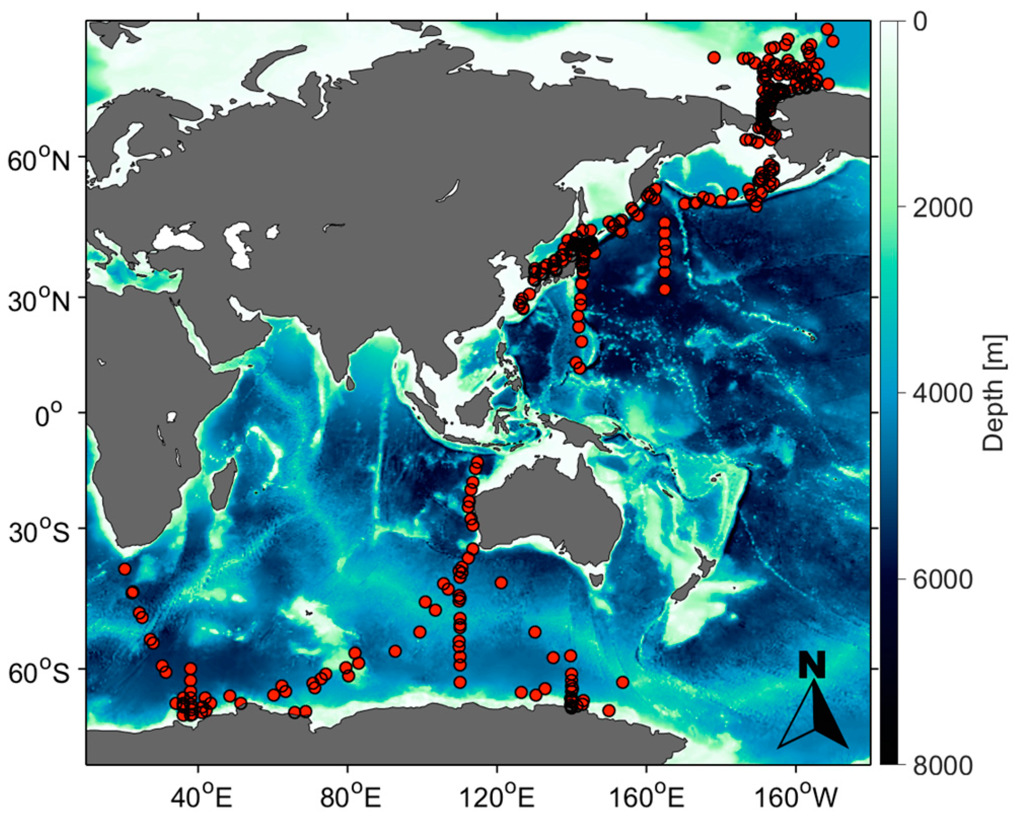
2.1. In Situ Data

The dataset used in this study was obtained from a wide area following 23 cruises over a 16-year period (Figure 1,

Table 1. Cruises information and number of data obtained during each cruises.

Cruise Period	Cruise	Vessel Names	Number of Data
			Water Sample	Spectral Radiation
22 November–12 December 2000	JARE-42	JMSDF Shirase	19	6
16–25 February 2002	JARE-43	JMSDF Shirase	10	9
25 January–9 February 2003	UM0203	T/S Umitaka-maru	15	14
22 February–6 March 2003	JARE-44	R/V Tangaroa	9	6
1–21 January 2005	UM0405	T/S Umitaka-maru	16	11
5–22 January 2006	UM0506	T/S Umitaka-maru	10	7
25 July–14 August 2007	OS180	T/S Oshoro-maru	20	20
27 December 2007–12 February 2008	UM0708	T/S Umitaka-maru	21	15
13–25 January 2009	UM0809	T/S Umitaka-maru	9	7
18 August–18 September 2009	KH-09-4	R/V Hakuho-maru	16	16
11 September–10 October 2009	MR09-03	R/V Mirai	12	12
3 June–7 July 2010	OS216	T/S Oshoro-maru	21	17
4 September–13 October 2010	MR10-05	R/V Mirai	28	28
9–11 May 2011	KT-11-07	R/V Tansei-maru	8	7
8 June–7 July 2011	OS229	T/S Oshoro-maru	25	24
17–18 June 2012	US260	T/S Ushio-maru	8	7
6–8 August 2012	US263	T/S Ushio-maru	10	8
13 September–2 October 2012	MR12-E03	R/V Mirai	12	12
23 June–17 July 2013	OS255	T/S Oshoro-maru	26	24
31 August–4 October 2013	MR13-06	R/V Mirai	32	32
10–12 October 2013	ARAON-EJS	Icebreaker ARAON	9	7
8–30 June 2014	Mu14	R/V Multanovski	16	16
8–23 March 2015	KH-15-1	R/V Hakuho-maru	12	12

). At each station, size fractionated Chla (Chla_size), light absorption coefficient, and spectral radiation were measured, the detailed procedures of which are described below. Note that the spectral radiation was not observed at some stations. Seawater samples were collected from the sea surface (0 m) using a clean plastic bucket. Seventy percent of in situ data were used for model development and the remainder was reserved for model validation.

2.1.1. Size Fractionated Chla Concentration

We used various filters (

Table 2. Summary of pore size of filters that were used to obtain Chla_size during each cruises.

Cruise	20 μm	10 μm	5 μm	2 μm	GF/F
JARE-42	×	×		×	×
JARE-43	×	×		×	×
UM0203	×	×		×	×
JARE-44	×	×		×	×
UM0405		×		×	×
UM0506		×		×	×
OS180	×		×		×
UM0708	×		×		×
UM0809		×		×	×
KH-09-4		×		×	×
MR09-03		×	×	×	×
OS216		×	×	×	×
MR10-05		×	×	×	×
KT-11-07		×	×	×	×
OS229		×	×	×	×
US260		×		×	×
US263		×		×	×
MR12-E03	×	×	×	×	×
OS255	×			×	×
MR13-06	×	×		×	×
ARAON-EJS	×			×	×
Mu14	×			×	×
KH-15-1	×			×	×

) to obtain Chla_size during each cruise. Seawater samples (n = 364) were filtered onto polycarbonate membrane or nylon mesh filters (20, 10, 5, and 2 μm pore size) and GF/F filters (Whatman, ca. 0.7 μm pore size) under low vacuum pressure (<0.013 MPa). After filtration, the filter was immediately soaked in N,N-dimethylformamide, and pigments were extracted for 24 h in the dark at −20 °C [26]. Chla concentrations were determined by the fluorescence acidification technique [27] during JARE-42, JARE-43, UM0203, 44Tangaroa and UM0405 and the non-acidification technique [28] during other cruises using a 10-AU fluorometer (Turner Designs Inc., San Jose, CA, USA).

2.1.2. Absorption Coefficient of Phytoplankton

To measure phytoplankton absorption spectra, particles in water samples were collected onto a GF/F filter. The optical density (OD) of particles on the filter was measured immediately after sampling using a MPS-2400 or a MPS-2450 spectrophotometer (Shimadzu, Japan) at wavelengths of 350–750 nm, and the absorption coefficient of the total suspended particles (a_p(λ)) was determined from the OD according to the quantitative filter technique [29]. The OD of the NAPs was then measured after soaking in methanol [30] or sodium hypochlorite [31], and the absorption coefficient of the NAPs (a_d(λ)) was quantified as well as a_p(λ). Finally, a_ph(λ) was obtained by subtracting a_d(λ) from a_p(λ).

2.1.3. Retrieval of IOPs from In Situ Spectral Radiation Data

In situ spectral distributions of the underwater radiation (n = 317) were acquired using a SMPR (Satlantic Inc., Halifax, NS, Canada), a HyperPro (Satlantic Inc., Halifax, NS, Canada) or a PRR-800/810 (Biospherical Instruments Inc., San Diego, CA, USA). The HyperPro measures underwater downward spectral irradiance (E_d(λ, z)) and upward spectral radiance (L_u(λ, z)) at 136 wavelengths between 350 and 800 nm. The SPMR and PRR-800/810 measures those radiations at 13 and 17 wavelengths between 400 and 705 nm and between 380 and 765 nm, respectively. These measurements were acquired at the same time as above-water measurements of downward spectral irradiance (E_ds(λ)) were taken using a sensor mounted on the ship deck.

Remote sensing reflectance (R_rs(λ)) was calculated as the ratio of the water-leaving radiance (L_w(λ)) to E_ds(λ):

$$R_{\mathrm{rs}}\left(\lambda \right)=L_{\mathrm{w}}\left(\lambda \right)/E_{\mathrm{ds}}\left(\lambda \right)$$

(1)

The L_w(λ) was obtained from L_u(λ, z) just beneath the water surface (L_u(λ, 0−), which was determined as the fitting coefficient of near-surface L_u(λ, z) and the water-air interface propagation factor of 0.544 [32] as follows:

$$L_{\mathrm{w}}\left(\lambda \right)=0.544\times L_{\mathrm{u}}\left(\lambda , 0-\right)$$

(2)

$$L_{\mathrm{u}}\left(\lambda , z\right)=L_{\mathrm{u}}\left(\lambda , 0-\right)\times \exp \left[-K_{\mathrm{u}}\times z\right]$$

(3)

where z and K_u(λ) are the depth and diffuse attenuation coefficient of upward radiance, respectively. Then, R_rs(λ) was resampled at 10 MODIS bands (412, 443, 469, 488, 531, 547, 555, 645, 667, and 678 nm) from the original wavelength of the spectroradiometers using spline interpolation [25]. To estimate a_ph(λ) from in situ R_rs(λ), the latest version of the quasi-analytical algorithm version 6 (QAA-v6) [33] was applied to the observed R_rs(λ).

2.2. Satellite Remote Sensing Data

MODIS-Aqua Level-3 standard mapped daily images of OC3M Chla and R_rs(λ) at 10 MODIS bands were downloaded from the Goddard Space Flight Center/National Aeronautics and Space Administration for 2003–2015. The temporal and spatial resolutions of these satellite data were daily and 9 km, respectively. The a_ph(λ) at the MODIS bands were derived from R_rs(λ) data using the QAA-v6. Daily Advanced Very High Resolution Radiometer Pathfinder Version 5.2 SST data with 4-km spatial resolution were obtained for 2003–2015 from the USA National Oceanographic Data Center/National Oceanic and Atmospheric Administration and the Group for High Resolution Sea Surface Temperature. The Pathfinder Version 5.2 data are an updated version of the Pathfinder Version 5.0 and 5.1 collections described in Casey et al. [34]. These satellite data were resampled on a 1° × 1° grid and composited as monthly averages to minimize local and transient variabilities.

2.3. Model Description

Assuming that the PSD follows the Junge-type [35] power law size distribution [36], the number of particles per unit volume (N) of seawater normalized by the size bin diameter (D), N(D), can be expressed as follows:

$$N\left(D\right)=N_0{\left(D/D_0\right)}^{-\xi }$$

(4)

where ξ is the Junge slope of the PSD, and D₀ is a reference diameter at which N₀ = N(D₀). Therefore, the total number of particles in a given size range can be derived by integrating Equation (4) from the minimum diameter (D_min) to the maximum diameter (D_max); thus, enabling the PSD to be partitioned into distinct classes described by

$$N=\underset{D_{\min }}{\overset{D_{\max }}{{\displaystyle \int }}}{N}_0{\left(D/D_0\right)}^{-\xi }dD$$

(5)

Given that the Chla is particulate, and thus the Chla size distribution (CSD) also follows the Junge-type power law distribution, the total Chla (Chla_total) and Chla_size in a given size range from D₁ to D₂ can be expressed using Equations (6) and (7) as follows:

$$\mathrm{Chl}{a}_{\mathrm{total}}=\underset{D_{\min }}{\overset{D_{\max }}{{\displaystyle \int }}}\mathrm{Chl}{a}_0{\left(D/D_0\right)}^{-\eta }dD$$

(6)

$$\mathrm{Chl}{a}_{\mathrm{size}}=\underset{D_1}{\overset{D_2}{{\displaystyle \int }}}\mathrm{Chl}{a}_0{\left(D/D_0\right)}^{-\eta }dD$$

(7)

where Chla₀ is the reference Chla at D₀ (here, 0.7 μm), and η is the exponent of the Chla size spectrum (hereafter, CSD slope). Larger magnitudes of the CSD slope indicate a large proportion of smaller phytoplankton, whereas smaller magnitudes suggest predominance of larger phytoplankton. In this study, we assumed D_min and D_max as the pore size of GF/F filter (i.e., nominal 0.7 μm) and 200 μm [37], respectively. The CSD slope is derived as the slope of the linear regression in log-space between the inverse log-transformed median diameters from log-transformed D₁ to D₂ and Chla_size normalized by the size bin width.

Note that the Chla fraction of an arbitrarily defined size range (F_size) can be derived using the CSD slope as follows:

$$F_{\mathrm{size}}=100\times \frac{\mathrm{Chl}{a}_{\mathrm{size}}}{\mathrm{Chl}{a}_{\mathrm{total}}}=100\times \frac{{{\displaystyle \int }}_{D_1}^{D_2}\mathrm{Chl}{a}_0{\left(D/D_0\right)}^{-\eta }dD}{{{\displaystyle \int }}_{0.7}^{200}\mathrm{Chl}{a}_0{\left(D/D_0\right)}^{-\eta }dD}=100\times \frac{D_2^{1-\eta }-D_1^{1-\eta }}{{200}^{1-\eta }-{0.7}^{1-\eta }}$$

(8)

where the constants Chla₀ and D₀ no longer exist in Equation (8), such that only the CSD slope and diameter range are required for estimating each fraction of the phytoplankton size classes.

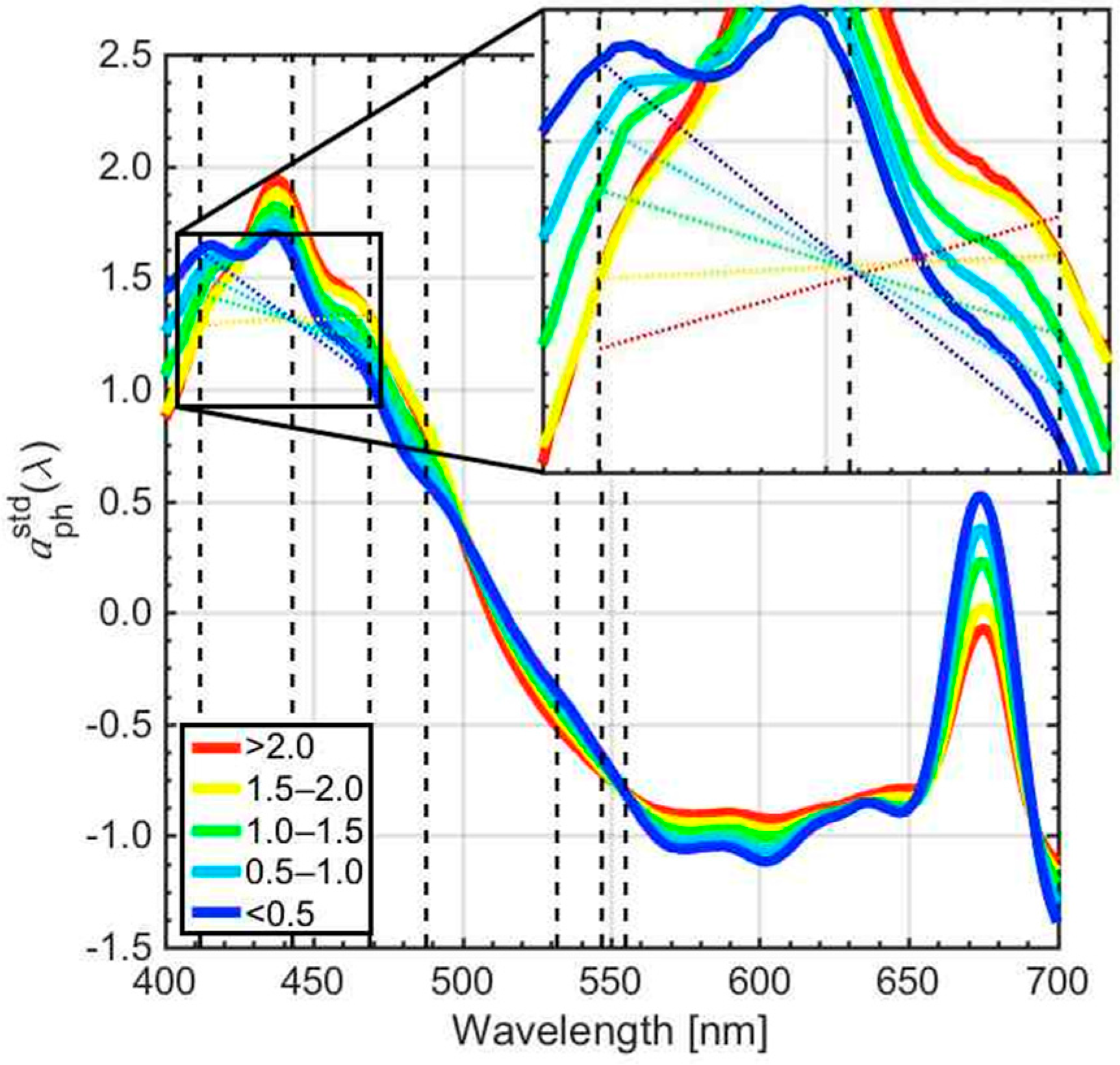
2.4. Quantification of CSD Slope Using Phytoplankton Absorption Spectra

To quantify the CSD slope using the spectral shape of a_ph(λ), we applied PCA to the normalized a_ph(λ), according to the method of Wang et al. [25]. In brief, the normalized a_ph(λ) ($a_{\mathrm{ph}}^{\mathrm{std}}$(λ)) was derived from the wavelength mean and standard deviation of a_ph(λ) at 10 MODIS bands. The formula for $a_{\mathrm{ph}}^{\mathrm{std}}$(λ) is shown below:

$$a_{\mathrm{ph}}^{\mathrm{std}}\left(\lambda \right)=\left[a_{\mathrm{ph}}\left(\lambda \right)-\mathrm{mean}\left(a_{\mathrm{ph}}\left(\lambda \right)\right)\right]/\mathrm{std}\left(a_{\mathrm{ph}}\left(\lambda \right)\right)$$

(9)

where mean(a_ph(λ)) and std(a_ph(λ)) are the wavelength mean and standard deviation of a_ph(λ), respectively. Then, PCA was applied to $a_{\mathrm{ph}}^{\mathrm{std}}$(λ) to capture the spectral features of the phytoplankton absorption properties. The input values for the PCA comprised a matrix (m × N) constituted of $a_{\mathrm{ph}}^{\mathrm{std}}$(λ), where m and N are the numbers of the wavelengths and samples, respectively. The resulting principal component (PC) scores were assumed to correlate with the CSD slope; hence, the CSD slope was quantified as a logistic-type regression model using the i-th PC score (S_i) and regression coefficients between the CSD slope and PC scores (β₀ and β_i) as follows:

$$\eta ={\left[{\beta }_0+\exp {\displaystyle \sum }_{i=1}^k{\beta }_i{S}_i\right]}^{-1}$$

(10)

where k is the number of PCs. Here, S_i can also be expressed as follows:

$$S_i={\displaystyle \sum }_{j=1}^m{w}_{i,j}{a}_{\mathrm{ph}}^{\mathrm{std}}\left({\lambda }_j\right)$$

(11)

where w_i,j and $a_{\mathrm{ph}}^{\mathrm{std}}$(λ_j) are the loading factors for the i-th PC and $a_{\mathrm{ph}}^{\mathrm{std}}$(λ) value at wavelength j, respectively. Therefore, we obtained an equation by replacing S_i in Equation (10) with Equation (11):

$$\eta ={\left[{\beta }_0+\exp {\displaystyle \sum }_{j=1}^m{C}_j{a}_{\mathrm{ph}}^{\mathrm{std}}\left({\lambda }_j\right)\right]}^{-1}$$

(12)

$$C_j={\displaystyle \sum }_{i=1}^k{\beta }_i{w}_{i,j}$$

(13)

Finally, the CSD slope is derived from Equation (12) using the model parameters of β₀ and C_j.

To avoid unrealistic values of the CSD slope, we defined the upper and lower limits of the CSD slope as 3.0 and 0.0, respectively. These limits mostly corresponded to 90% of pico- and microplankton dominance to total Chla.

2.5. Evaluation of Estimate Accuracy

The relative root mean square error (RRMSE) was adopted when we validated the agreement of two values, such as the measured and estimated CSD slope. The RRMSEs were computed as relative values to provide equal weights to all samples and then expressed as percentages [38,39], as described by

$$\mathrm{RRMSE}(\%)=100\times \sqrt{\frac{1}{N}{\displaystyle \sum }_{i=1}^N{\left(\frac{Mea{s}_i-Mo{d}_i}{Mea{s}_i}\right)}^2}$$

(14)

where Meas_i and Mod_i are the i-th measured and modeled values, respectively.

2.6. Velocities of the Shift in Oceanographic Parameters

Velocities of the CSD slope, Chla, and SST were derived following the method of Burrows et al. [9]. The velocity along angle θ (V_θ), with 0° as North and 180° as South, was calculated on a 1° grid by dividing the temporal trend over the period 2003–2012 by the spatial gradient as follows:

$$V_{\theta }=\frac{\mathrm{Temporal}\mathrm{trend}}{\mathrm{Spatial}\mathrm{gradient}}$$

(15)

The long-term temporal trend was calculated as the slope of the linear regression between monthly anomalies and time. Note that the temporal trend was employed as an absolute value when we determined the velocity using Equation (15) to clarify the local speed of shifting contours. The spatial gradient was derived as the vector sum of the North–South and West–East spatial gradients of 3 × 3 neighborhoods, with the associated vector angle given by the direction of the gradient, as described by

$$\mathrm{Spatial}\mathrm{gradient}=S_{NS}\cos \theta +S_{EW}\sin \theta$$

(16)

where S_NS is the North–South spatial gradient and S_EW is the East–West spatial gradient. The North–South spatial gradient was calculated as the difference in the temporal average for each northern and southern adjacent pair divided by the distance between them. The West–East spatial gradient was calculated similarly for each western and eastern adjacent pair divided by the distance between the cells in each pair.

3. Results

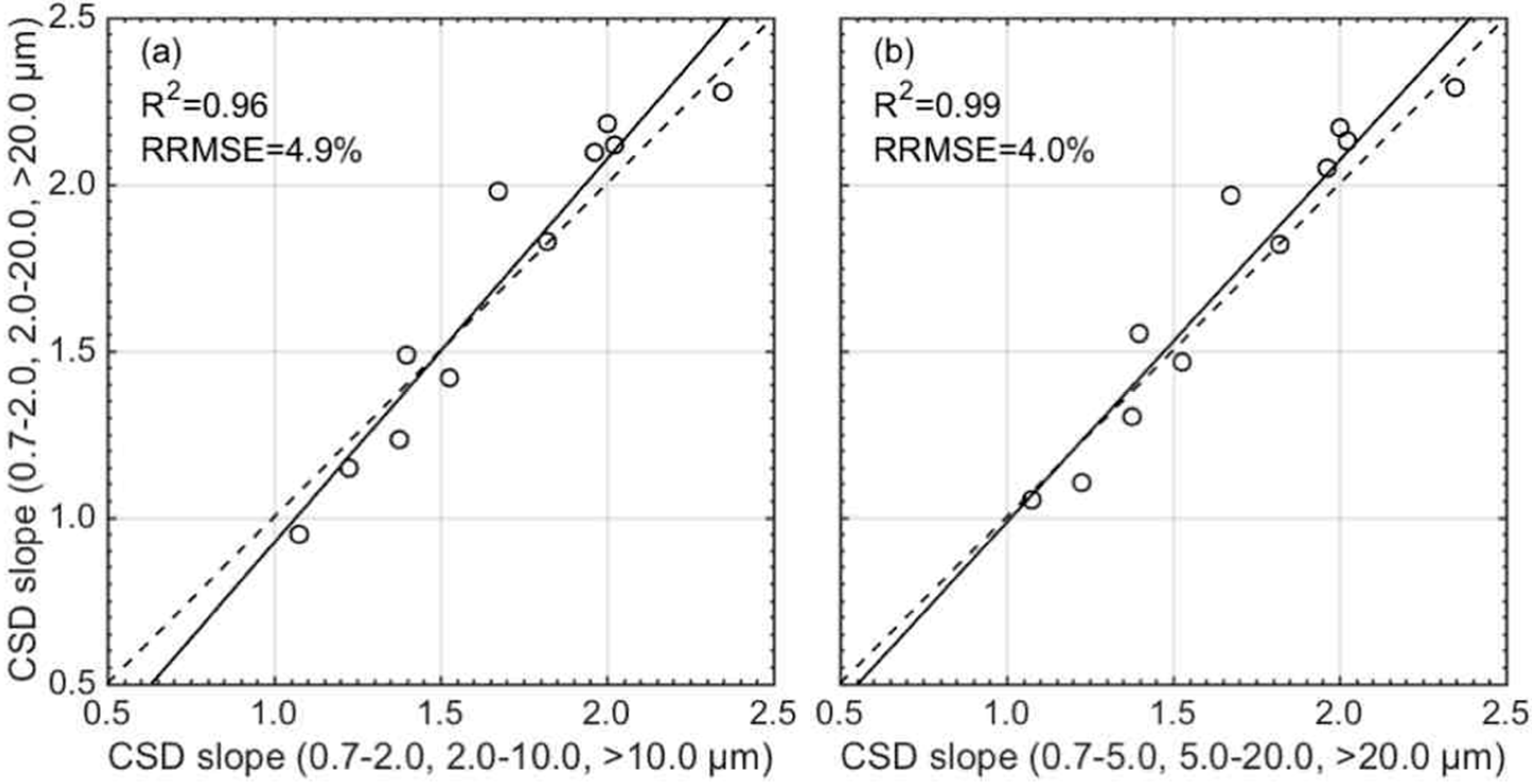
3.1. Retrieval of the CSD Slope from In Situ Chla_size

Various filters were used to obtain Chla_size (Table 2). In general, phytoplankton is partitioned into three size classes: picoplankton (0.7–2.0 μm), nanoplankton (2.0–20.0 μm) and microplankton (>20.0 μm). However, we have not used filters for dividing phytoplankton into the size classes during some cruises (e.g., UM0405, OS180 and KH-0904). This fact forces us to employ specific combinations of filters used for obtaining Chla_size, resulting in only a part of our dataset can be used together. Thus, our dataset could not be used in its entirety with typical methods such as Brewin et al. [40] and Devred et al. [41] that need to fix the size range of each phytoplankton size class. In contrast, it is possible to derive the CSD slope from any combination of Chla_size; hence, we succeeded in developing a CSD model using the entire dataset.

To verify the robustness of the CSD slope values determined by various combinations of filters, the CSD slopes derived from different combination of Chla_size were compared. For this comparison, the data obtained during the MR12-E03 cruise were employed because filters with various pore sizes were used during this cruise. Figure 2 shows the relationships between the CSD slope values derived from three typical Chla_size (0.7–2.0, 2.0–20.0, and >20.0 μm) and different combination of Chla_size. The resulting RRMSEs were 4.9% and 4.0%, and therefore we concluded that the differences in the CSD slope among the combinations of filters were negligible.

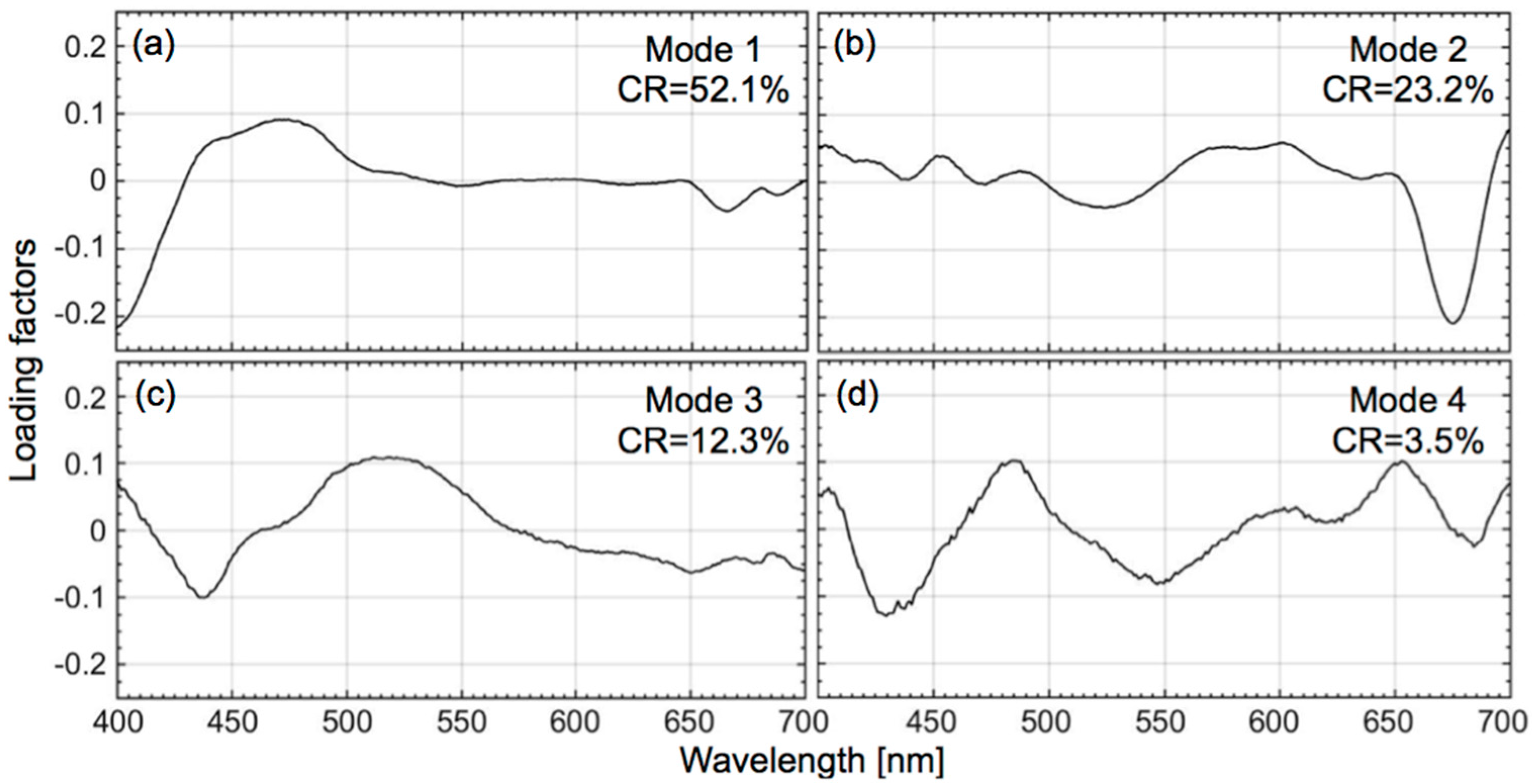
3.2. Empirical Development of the CSD Model

The method described in Section 2.3 was applied to our dataset for developing the CSD model. The in situ CSD slope ranged from 0.417 to 2.427. Note that smaller CSD slope values indicate phytoplankton assemblages with larger sizes, and vice versa. Figure 3 shows the relationship between the CSD slope and spectral shape of $a_{\mathrm{ph}}^{\mathrm{std}}$(λ). It is clear that there are remarkable differences in $a_{\mathrm{ph}}^{\mathrm{std}}$(λ) accompanying the variation of CSD slope. For instance, smaller CSD slope values show remarkably higher values of $a_{\mathrm{ph}}^{\mathrm{std}}$(λ) between 400 and 430 nm than do larger values of the CSD slope. In addition, $a_{\mathrm{ph}}^{\mathrm{std}}$(λ) values associated with smaller CSD slope values are higher than those of larger CSD slope values between 660 and 690 nm. These differences in $a_{\mathrm{ph}}^{\mathrm{std}}$(λ) were mainly due to a coupling of the packaging effect and pigment composition, which is strongly affected by phytoplankton cell size and species composition [25]. Overall, the results were generally consistent with Ciotti et al. [42] and Wang et al. [25].

To capture the spectral differences in $a_{\mathrm{ph}}^{\mathrm{std}}$(λ), PCA was conducted using $a_{\mathrm{ph}}^{\mathrm{std}}$(λ) between 400 and 700 nm with 1-nm resolution. The first four PC modes explained >94.2% of the total variance in $a_{\mathrm{ph}}^{\mathrm{std}}$(λ) and the first mode captured 52.1%. The spectral shape of the first mode indicates negative loading factor between 400 and 430, and 660 and 690 nm and positive loading factor between 430 and 550 nm (Figure 4a). The second mode explained 23.2% of the total variance and the spectrum shows an obvious negative peak between 660 and 690 nm (Figure 4b). The third mode explained 12.3% of the total variance in $a_{\mathrm{ph}}^{\mathrm{std}}$(λ). This mode shows a monotonous decrease from 400 to 430 nm, followed by an increase above 500 nm (Figure 4c). The fourth mode explained only 3.5% of the total variance; several positive and negative peaks are evident in the spectral shape (Figure 4d).

These spectral features derived from PCA can be interpreted as signatures of changes in $a_{\mathrm{ph}}^{\mathrm{std}}$(λ). However, ocean color sensors restrict us to using only specific numbers of wavelengths for PCA because of the limitation of available observation bands. Although additional wavelengths are better for a PCA approach, previous studies have reported that reduced wavelength information has little influence on model performance [23,25]. Initially, we attempted to conduct PCA for $a_{\mathrm{ph}}^{\mathrm{std}}$(λ) resampled at 10 MODIS bands between 400 and 700 nm; however, the estimation accuracy of the QAA-v6 became quite poor at longer wavelengths such as 645, 667, and 678 nm with huge RRMSE values of 67.2%, 77.9%, and 58.1%, respectively (

Table 3. Summary of performances of the QAA-v6 at 10 MODIS bands. R² and RRMSE were calculated in log10 space using full dataset (n = 317) after omitting minus values.

	Wavelength (nm)
	412	443	469	488	531	547	555	645	667	678
Number of minus value	31	31	36	28	78	77	86	14	44	83
R2	0.68	0.71	0.59	0.61	0.57	0.62	0.57	0.00	0.01	0.01
RRMSE (%)	20.3	19.0	19.7	21.2	20.5	15.8	15.4	67.2	77.9	58.1

). Therefore, only a_ph(λ) at the seven shorter wavelengths of 412, 443, 469, 488, 531, 547, and 555 nm were used for developing our CSD model.

The first four PC scores derived from $a_{\mathrm{ph}}^{\mathrm{std}}$(λ) at the seven wavelengths and the CSD slope were used to fit the logistic-type function, following which the model parameters β₀ and C_j were determined. Comparison of the CSD slopes derived from in situ Chla_size and in situ a_ph(λ) shows good agreement (RRMSE: 17.4%); however, data scattering for higher CSD slope values is apparent (Figure 5a). This might be because one combination of regression coefficients cannot capture the entire relationship between the phytoplankton size structure and the spectral shape of a_ph(λ). When focusing on the average $a_{\mathrm{ph}}^{\mathrm{std}}$(λ) at the MODIS bands, the $a_{\mathrm{ph}}^{\mathrm{std}}$(λ) at 412 nm was higher than at 469 nm for smaller CSD slopes, and vice versa. These spectral features were also found in previous studies, and they were attributed to differences in pigment composition related to phytoplankton cell size [42]. For such practical considerations, we divided the dataset for model development into two, according to the relationship between $a_{\mathrm{ph}}^{\mathrm{std}}$(λ) at 412 and 469 nm, and then determined the model parameters for each dataset. Thus, the CSD model is defined as summarized in

Table 4. Model parameters (β₀ and C_j in Equation (12)) for CSD slope estimation.

	Model Parameters
	β0	C1	C2	C3	C4	C5	C6	C7
aph(412) ≥ aph(469)	−0.221	0.324	0.021	−0.780	0.243	1.714	−0.190	−1.308
aph(412) < aph(469)	−0.314	0.245	0.026	−0.693	0.209	1.813	−0.191	−1.311

. The resulting relationship between in situ and modeled CSD slopes shows better agreement (Figure 5b), for which the RRMSE was reduced significantly to 13.2%. Note that sampling locations of these two dataset were randomly distributed in latitude and longitude, suggesting geographic bias seemed negligible. We also tried to quantify CSD slope based on previous methods described in Kostadinov et al. [17], Brewin et al. [40], and Fujiwara et al. [18], for which the resulting RRMSEs were 31.6%, 31.7%, and 31.8%, respectively. These results suggest that the PCA approach is superior to other methods in the quantification of CSD slope.

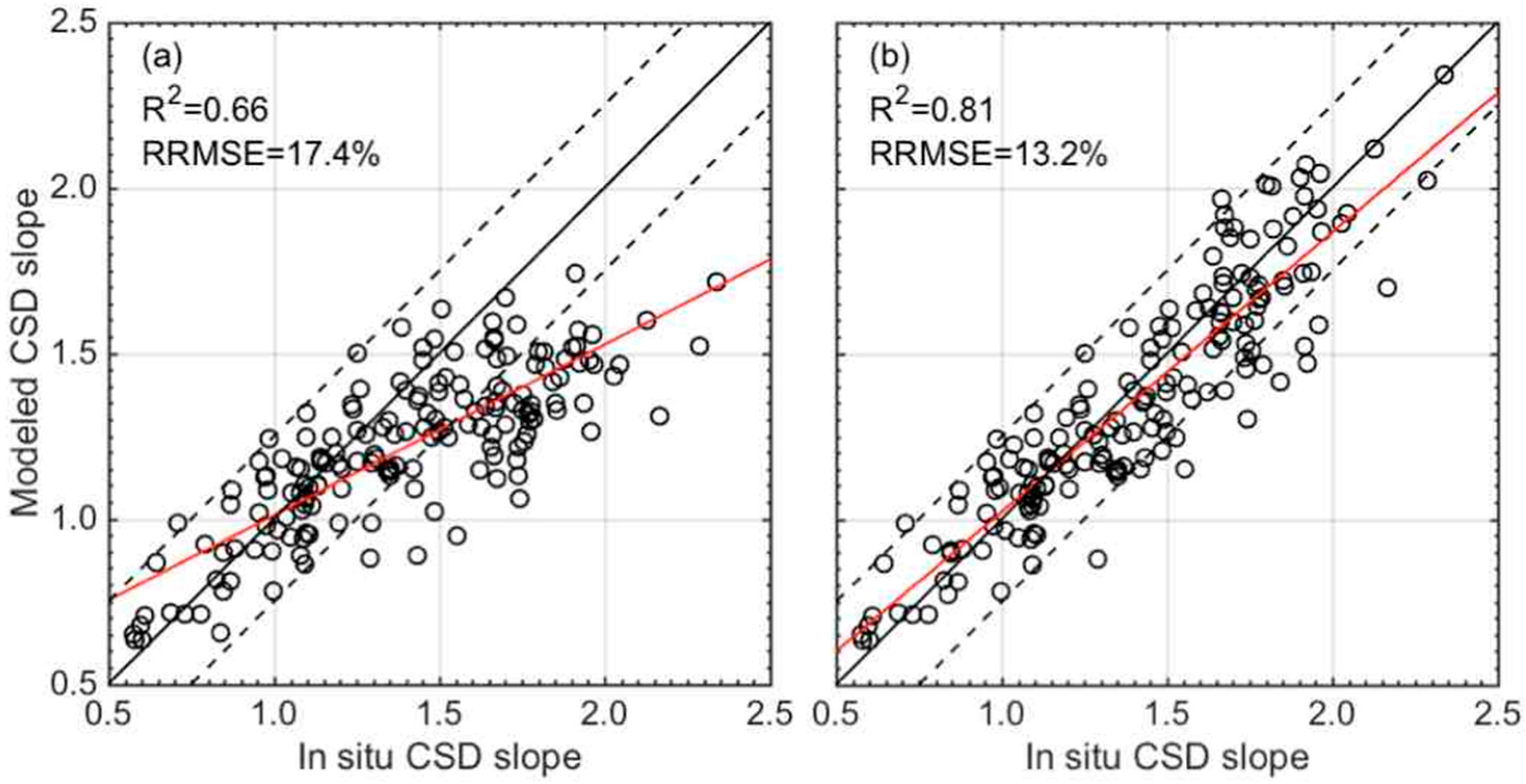
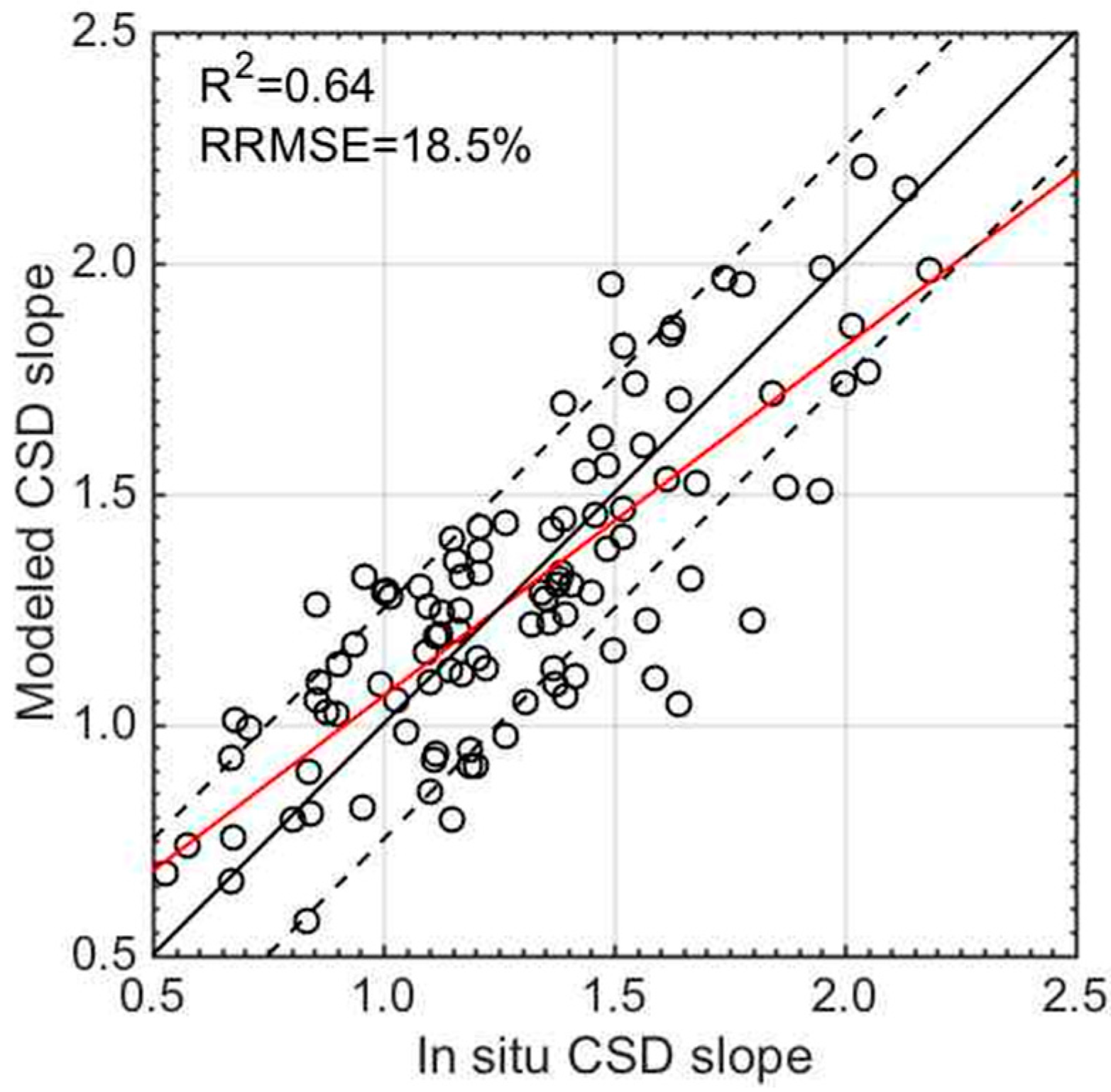
3.3. Validation of the CSD Model

The performance of the CSD model was examined by comparing measured CSD slope values determined from in situ Chla_size and modeled CSD slope values estimated from in situ R_rs(λ). The resulting RRMSE between the measured and modeled CSD slope values was 18.5% (Figure 6). As the CSD model relies on the spectrum shape of a_ph(λ), the accuracy of the modeled CSD slope values depends strongly on the robustness of the IOP algorithms. Therefore, the performance of the CSD model will be improved when IOP algorithms that are more robust are developed. However, the CSD model successfully retrieved the CSD slope within ±0.25 ranges for 75 out of 106 (70.8%) validated data. Thus, we considered that the CSD model performed with sufficient accuracy for assessing the CSD slope; hence, it could be used to derive global estimations of phytoplankton size structure.

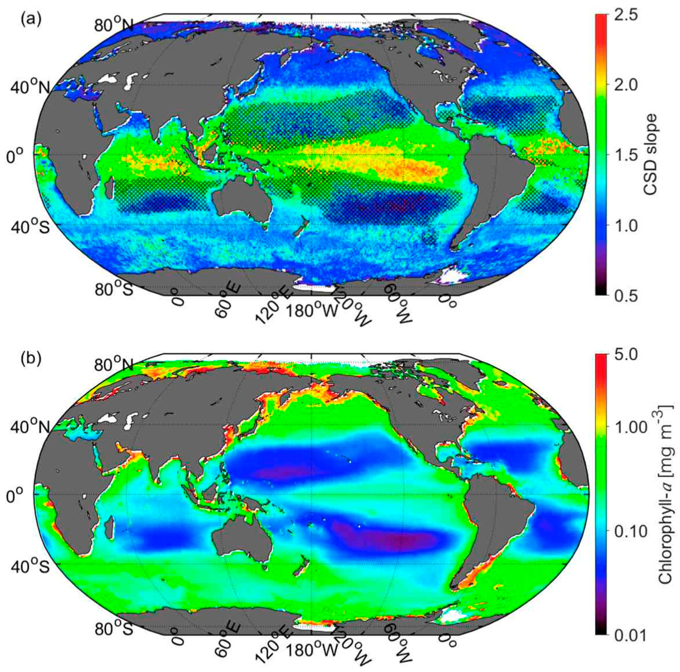
3.4. Global Distribution of CSD Slope and Chla

Figure 7 shows the average CSD slope and Chla values during the period from January 2003 to December 2015. It can be seen that smaller CSD slope values are present in coastal upwelling regions such as in the areas of the Benguela and Humboldt currents, whereas larger CSD slope values are found in oligotrophic regions, especially the equatorial regions. In general, these global patterns of CSD slope exhibit an inverse relationship with Chla, suggesting areas of high and low productivity are associated with the relative dominance of larger and smaller phytoplankton assemblages, respectively. However, smaller CSD slope values are also evident in areas of low productivity, such as subtropical gyres. This is because the total absorption coefficient was close to that of pure seawater and the estimated IOPs include large errors, resulting in huge uncertainties regarding the performance of the CSD model.

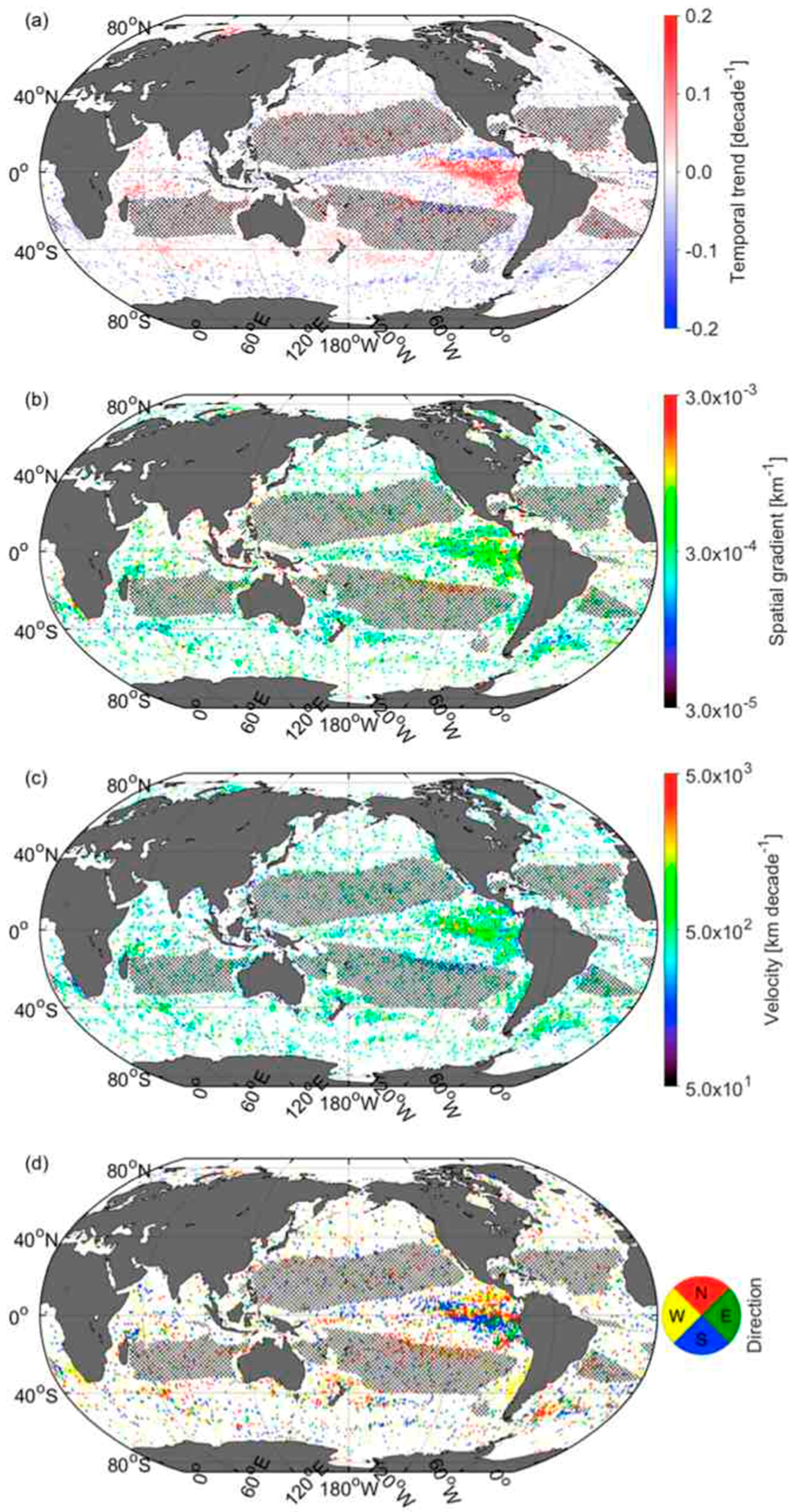
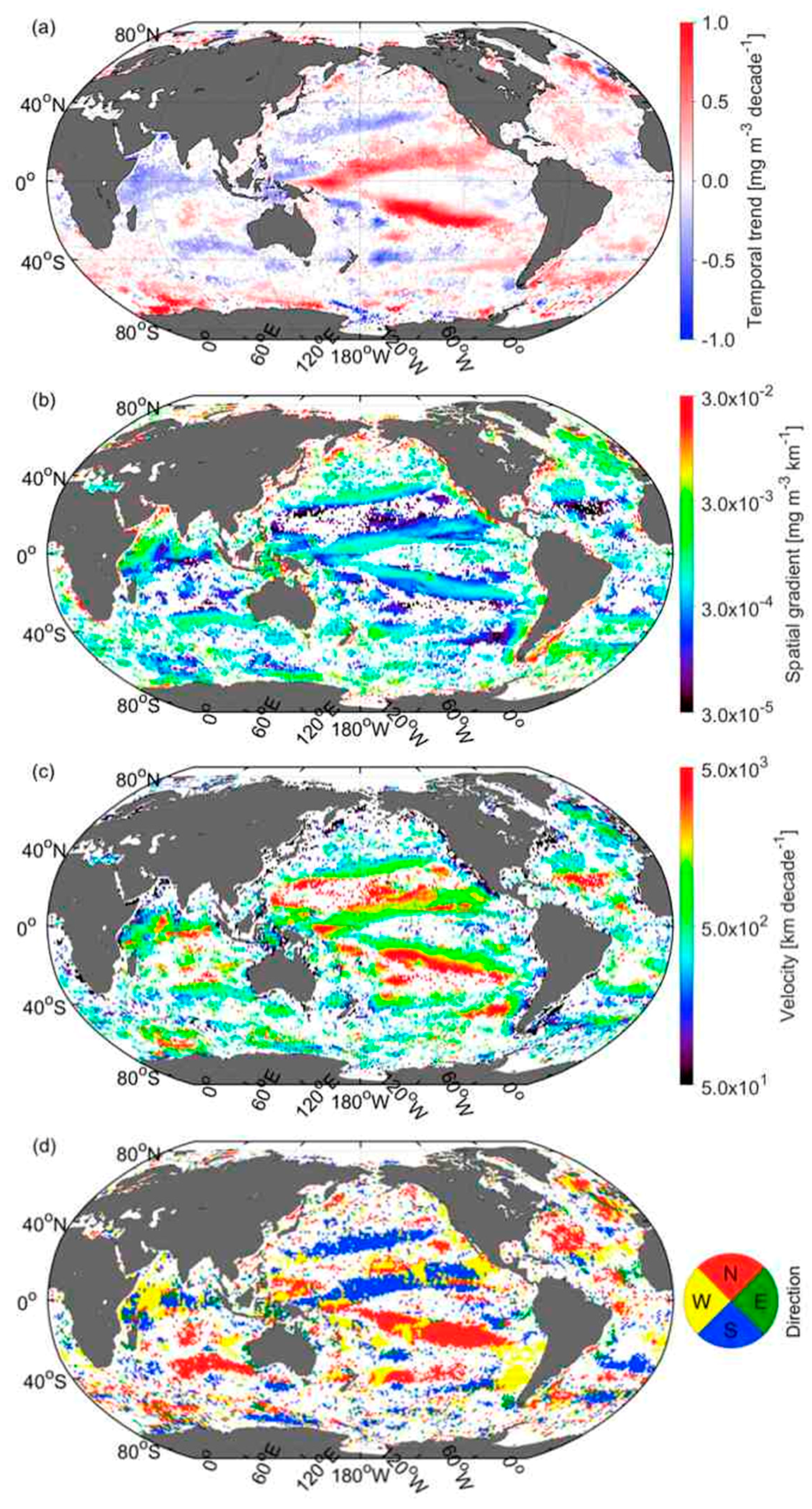
3.5. Velocities of Shift in CSD Slope and Chla

The temporal trend of CSD slope values was derived as a simple linear regression slope of the monthly anomaly of CSD slope against time (Figure 8a). Overall, 20.1% of the global oceans had significant increases or decreases (p < 0.05) during 2003–2015. An increasing trend in CSD slope, indicating a change toward a smaller phytoplankton community, was found for 57.4% of these regions. A significant increasing or decreasing trend in Chla was found in 54.8% of the global oceans for 2003–2015 (Figure 9a), with 63.6% of these regions exhibiting a decreasing trend. The spatial gradient of CSD slope was relatively large along coastal regions and subtropical gyres result from dynamic changes in CSD slope with modest spatial displacements (Figure 8b). This global pattern of spatial gradient was consistent with that of Chla (Figure 9b). However, it should be noted that the large estimation error of CSD slope was substantial in areas of low productivity. As a clear temporal trend in Chla was found in these regions, the biogeochemical and ecological processes within these regions are likely to have experienced climate forcing. Therefore, accurate estimation of the phytoplankton size structure would contribute to improved understanding of the changes in these processes by providing information that is more detailed than provided by the spatiotemporal variability of Chla.

It appeared that the velocities of CSD slope and Chla depended strongly on their spatial gradients rather than on their temporal trends because the velocities showed clear inverse distributions with the spatial gradients. When the rates of temporal change and spatial gradient of the CSD slope were combined, the resulting median velocity of the CSD slope across the ocean was 485.2 km·decade⁻¹ (Figure 8c). This value is largely consistent with that of 531.5 km·decade⁻¹ for Chla (Figure 9c). These velocities are equivalent to the observed distribution shift of the phytoplankton community (469.9 ± 115.3 km·decade⁻¹) reported by Poloczanska et al. [12]. The directions of shifts both in CSD slope (Figure 8d) and in Chla (Figure 9d) show a mosaic distribution, suggesting that spatiotemporal variations of CSD slope and Chla are non-uniform across the oceans. As species response to climate forcing is specific to the regional scale [6], a complex mosaic of the spatiotemporal variations of CSD slope and Chla has the potential for providing assessments of shifts in species distributions that are more accurate.

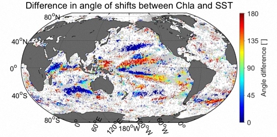
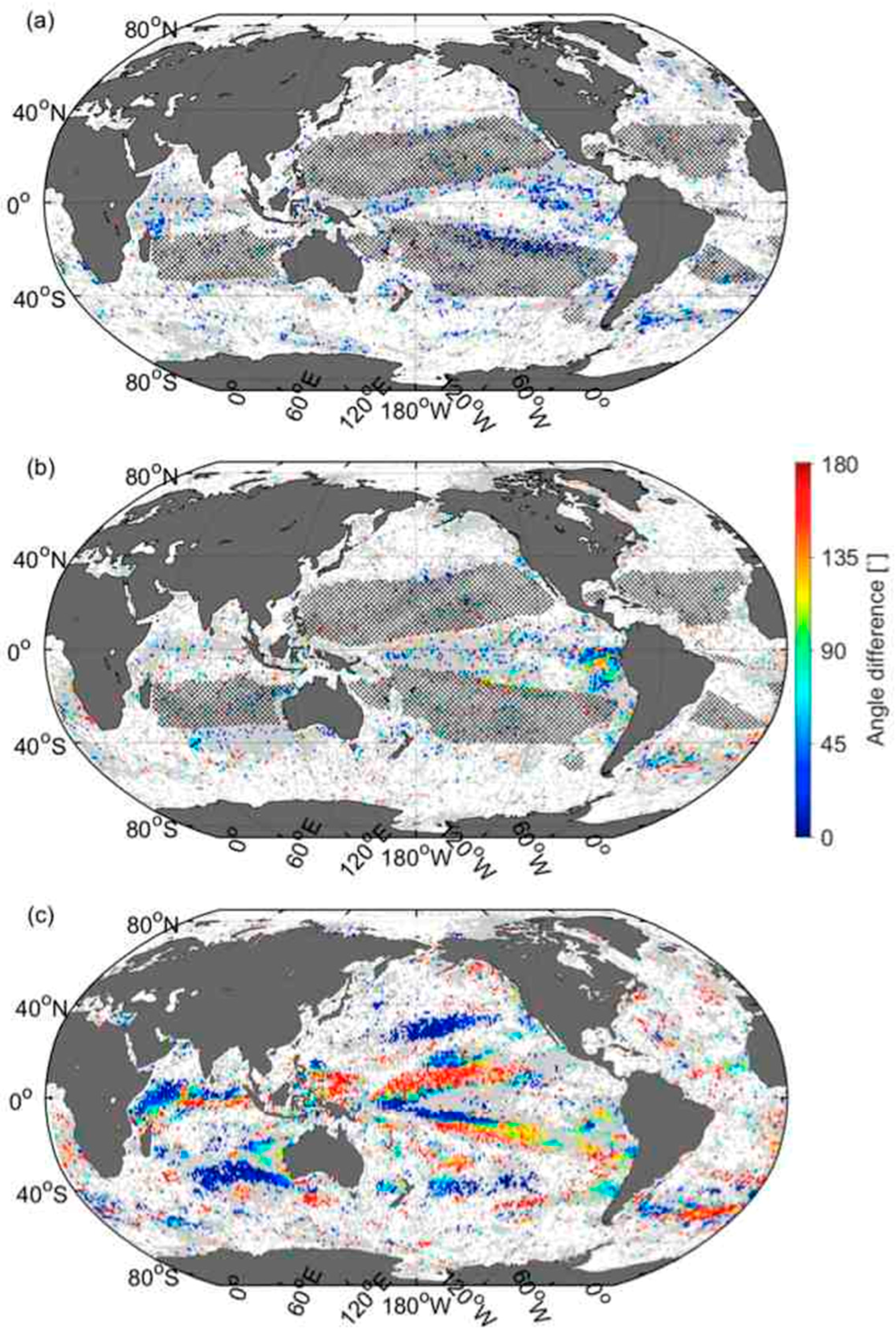
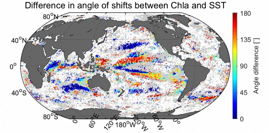
3.6. Comparison of Velocities Derived from CSD Slope and Chla with That of SST

The SST shows significant temporal change in 34.9% of the global oceans, of which regions of warming and cooling account for 78.4% and 21.6%, respectively (Figure 10a). The global median velocity of SST was 292.8 km·decade⁻¹ and this is approximately half that of the CSD slope and Chla (Figure 10c), suggesting a modest movement of the isotherms compared with the shifts in CSD slope and Chla. Note that the velocity of SST in this study was more than 10 times that reported in Burrows et al. [9] (21.7 km·decade⁻¹). This discrepancy was caused by differences in methods; i.e., this study used only statistically significant trends (p < 0.05), and non-significant trends that result in low velocities were excluded. In fact, the median velocity of SST in this study was 35.3 km·decade⁻¹ when both significant and non-significant trends were included.

Although the direction of shift in SST also shows a complex pattern, which clearly differs from a simple poleward migration (Figure 9d), there are clear regional differences in the directions of velocities among the CSD slope, Chla, and SST (Figure 11). For instance, the directions of shifts in CSD slope and Chla are largely consistent (Figure 11a), whereas the direction of shift in SST deviates from those of CSD slope (Figure 11b) and Chla (Figure 11c). The direction of shift in SST shows a patchy pattern in which some areas are comparable and others dissimilar to those of both CSD slope and Chla, and specific patterns were not found in this study. Thus, the rates and directions of shifts in CSD slope and Chla could explain the variations in species distribution that deviate from that of SST [12,13].

4. Discussion

Satellite-based estimation of spatiotemporal variation in phytoplankton size structure can contribute to better understanding of the biogeochemical and ecological responses to recent climate forcing [14]. In this study, we developed a CSD model based on empirical relationships between the size distribution of Chla and the spectral shape of a_ph(λ). This method enabled us to derive with sufficient accuracy the synoptic size structure of the phytoplankton community using satellite remote sensing, based on our dataset obtained from a wide area of the North Pacific, Southern Ocean and Western Arctic oceans (Figure 1), despite approximately one third the samples being obtained from the optically complex waters of the Western Arctic Ocean [43,44]. We should note that the global distribution of CSD slope includes uncertainties in clear waters due to the estimation error in a_ph(λ) by QAA. Although other IOP algorithms for a_ph(λ) estimation such as the Garver–Siegel–Maritorena model [45] and the Constrained Liner Matrix model [46] might perform well, even in the clearest waters, the fixed shape estimation of a_ph(λ) is not applicable to our CSD model. Because the model relies strongly on the estimated spectrum of a_ph(λ), which is derived from the water-leaving radiance through an IOP algorithm [25], the performance of the CSD model, especially in clear waters, will be improved when IOP algorithms that are more robust are developed.

Compared with existing models, our CSD model has several advantages. First, this model is applicable to both coastal and open waters. Although some models [47,48] use the spectral features of R_rs(λ), which are affected strongly by non-algal components [20] and hence restricted to application in open waters, our CSD model has been developed using a_ph(λ), which is separated from the absorption by colored dissolved organic matter and NAPs [22]. Second, the CSD model can avoid the estimation errors of a_ph(λ) because our method requires a_ph(λ) at shorter wavelengths (i.e., between 412 and 555 mm), while the model proposed by Roy et al. [19] depends on the accuracy of the a_ph(676) estimation, which generally contains significant error because of strong absorption by pure seawater [22]. Third, the use of the spectral shape of a_ph(λ) enables us to reduce the influence of non-algal components, whereas the b_bp(λ)-based approach [17] can be affected not only by phytoplankton but also by all other suspended particles [21]. In addition, the fraction of user-defined phytoplankton size classes can be derived with the CSD model according to Equation (8), while most other models can retrieve only predefined size classes. Furthermore, the CSD model has been developed using Chla_size, which was determined by size-fractionated filtration. Although diagnostic pigment analysis (DPA) is frequently applied to classify phytoplankton size classes based on the photosynthetic pigment composition [19,25,39,40,49], Brewin et al. [50] reported that the DPA method had significant uncertainties. Therefore, we believe that the size-fractionated filtration-based method could be useful for obtaining phytoplankton size structures that are more accurate. Finally, the CSD model can represent the synoptic size structure of the phytoplankton community with one component, and hence the CSD slope is easily applicable to ocean biogeochemical models for retrieving phytoplankton size structures, which provide a useful index of the trophic status of the water mass, efficiency of the biological pump, and productivity of the marine ecosystem.

It has been well documented that the relationship between the size structure and abundance of the phytoplankton community shows strong covariance [39,40,49]; i.e., the fractional contribution of microplankton to Chla increases monotonically with increasing Chla, and vice versa. Indeed, the regional distribution of CSD slope showed a clear inverse pattern to that of Chla. Additionally, our demonstration of the temporal trend in Chla showed regional patterns of increase and decrease for the period 2003–2015, as reported in previous studies [51,52], and the distribution of CSD slope was generally the inverse. These results suggest that Chla and phytoplankton size structure are strongly covariant, and hence we consider that Chla could become an index of phytoplankton size structure. However, the regions where CSD slope and Chla showed statistically significant trends were quite limited. This is because the statistically significant regions of CSD slope were scarce in comparison with Chla. For instance, Chla showed significant increases or decreases in large parts of oligotrophic regions, where valid CSD slopes could not be retrieved because of the low estimation accuracy of the QAA-derived a_ph(λ). Therefore, a robust a_ph(λ) estimation in clear waters is an urgent requirement for the CSD model, as are other IOP-based approaches, for improved understanding of ecological and biogeochemical changes in these regions.

Species distributional shifts have been reported for a variety of organisms such as mollusks, fish, birds, and mammals [3,53], and their shifts have often been linked to temperature increases as expectations include simple poleward distribution shifts [54,55]. However, in terms of a warming perspective, unexpected equatorward and shallower migrations have been observed [56,57]; thus, the complex mosaic of local velocity of SST (Figure 10c,d) is believed to represent a powerful tool for evaluating the variability in species distribution [9]. Recent studies have applied the velocity of SST to the expectation of species range shifts [12,13]. They found that some distributional shifts could be explained clearly by the velocity of SST, whereas others showed independent changes, attributable to the different sensitivities and strategies of marine organisms [11]. VanDerWal et al. [10] reported that the expectation of shifts in species distributions driven by temperature alone is likely to underestimate the actual shifts. Moreover, Sunday et al. [58] revealed that the velocity of SST explained some of the variation in the range of shifts; however, including species traits more than doubled the explained variation. These facts suggest that adopting an approach that is more practical than the velocity of SST is required for better prediction of species shifts.

Trophic transfer efficiency describes the efficiency with which energy is transferred from one trophic level to the next [15] and it might control species distribution through changes in the food web structure [16]. As the size structure of the phytoplankton community can have considerable effect in determining trophic transfer efficiency [15], the spatiotemporal variations of CSD slope and Chla are considered as important factors that could potentially cause species distribution shifts. In this study, both the rates and directions of the velocities of CSD slope and Chla showed clear regional differences with those of SST. These findings imply that the velocities of CSD slope and Chla could constitute powerful tools for predicting species distribution shifts that deviate from isothermal movement. Furthermore, an approach that combines the velocity of phytoplankton size structure with SST might contribute to predictions of species distribution shifts that are more accurate than existing approaches, which consider only variations in species thermal niches.

Numerous time series are currently being stored with the aim of monitoring the effects of climate change. Although species responses to climate change have been extremely variable across ocean regions and taxonomic groups [12,59], understanding the pattern of variation and identifying where and when species will respond to climate forcing is essential if we are to manage proactively changes in fisheries resources and to meet conservation goals [58]. In consequence, as large proportions of species within marine ecosystems undergo distributional shifts [60], the provision of a cost-effective and relatively rapid integrated assessment of such shifts will be required [61]. Therefore, techniques for assessing species distribution shifts are currently garnering considerable attention [62,63]. In addition to the challenges involved in predicting species shifts, large gaps remain in our knowledge of species responses to climate change. This study provides compelling evidence regarding the potential for using phytoplankton size structure in assessing the persistence and migration of species distributions, which could contribute to the generation of global and regional maps of the expected rates and directions of species shifts that have improved accuracy.

5. Conclusions

This study proposed a CSD model to derive the synoptic size structure of the phytoplankton community using satellite remote sensing data. The CSD model is based on the relationship between phytoplankton size structure and its spectral absorption properties. The validation results showed that the CSD model performed with sufficient accuracy. Although satellite-derived CSD slope contains uncertainties, especially in clear waters, the CSD model has been demonstrated as a powerful tool for monitoring marine ecosystems through the synoptic size structure of the phytoplankton community. Recent evident deviations from uniform species shifts appear related to various environmental drivers, suggesting that a multifaceted approach, rather than using the velocity of SST, is probably required to assess species migration and persistence properly. Therefore, a new approach combining the velocity of phytoplankton size structure with other factors, including the velocity of SST, might contribute toward producing predictions of species distribution shifts with improved accuracy. Overall, our results could help generate global and regional maps of the expected rates and directions of species shifts.

References

1. Levitus, S.; Antonov, J.I.; Boyer, T.P.; Locarnini, R.A.; Garcia, H.E.; Mishonov, A.V. Global ocean heat content 1955–2008 in light of recently revealed instrumentation problems. Geophys. Res. Lett. 2009, 36, 1–5. [Google Scholar] [CrossRef]
2. Wassmann, P.; Kosobokova, K.N.; Slagstad, D.; Drinkwater, K.F.; Hopcroft, R.R.; Moore, S.E.; Ellingsen, I.; Nelson, R.J.; Carmack, E.; Popova, E.; et al. The contiguous domains of Arctic Ocean advection: Trails of life and death. Prog. Oceanogr. 2015, 139, 42–65. [Google Scholar] [CrossRef]
3. Grebmeier, J.M.; Bluhm, B.A.; Cooper, L.W.; Danielson, S.L.; Arrigo, K.R.; Blanchard, A.L.; Clarke, J.T.; Day, R.H.; Frey, K.E.; et al. Ecosystem characteristics and processes facilitating persistent macrobenthic biomass hotspots and associated benthivory in the Pacific Arctic. Prog. Oceanogr. 2015, 136, 92–114. [Google Scholar] [CrossRef]
4. Mueter, F.J.; Litzow, M.A. Sea ice retreat alters the biogeography of the Bering Sea continental shelf. Ecol. Appl. 2008, 18, 309–320. [Google Scholar] [CrossRef] [PubMed]
5. Spencer, P.D. Density-independent and density-dependent factors affecting temporal changes in spatial distributions of eastern Bering Sea flatfish. Fish. Oceanogr. 2008, 17, 396–410. [Google Scholar] [CrossRef]
6. Thackeray, S.J.; Sparks, T.H.; Frederiksen, M. Trophic level asynchrony in rates of phenological change for marine, freshwater and terrestrial environments. Glob. Chang. Biol. 2010, 16, 3304–3313. [Google Scholar] [CrossRef]
7. Dawson, T.P.; Jackson, S.T.; House, J.I.; Prentice, I.C.; Mace, G.M. Beyond Predictions: Biodiversity Conservation in a Changing Climate. Science 2011, 332, 53–58. [Google Scholar] [CrossRef] [PubMed]
8. Loarie, S.R.; Duffy, P.B.; Hamilton, H.; Asner, G.P.; Field, C.B.; Ackerly, D.D. The velocity of climate change. Nature 2009, 462, 1052–1055. [Google Scholar] [CrossRef] [PubMed]
9. Burrows, M.T.; Schoeman, D.S.; Buckley, L.B.; Moore, P.; Poloczanska, E.S.; Brander, K.M.; Brown, C.; Bruno, J.F.; Duarte, C.M.; Halpern, B.S.; et al. The Pace of Shifting Climate in Marine and Terrestrial Ecosystems. Science 2011, 334, 652–655. [Google Scholar] [CrossRef] [PubMed] [Green Version]
10. VanDerWal, J.; Murphy, H.T.; Kutt, A.S.; Perkins, G.C.; Bateman, B.L.; Perry, J.L.; Reside, A.E. Focus on poleward shifts in species’ distribution underestimates the fingerprint of climate change. Nat. Clim. Chang. 2012, 3, 239–243. [Google Scholar] [CrossRef]
11. Philippart, C.J.M.; Anadon, R.; Danovaro, R.; Dippner, J.W.; Drinkwater, K.F.; Hawkins, S.J.; Oguz, T.; O’Sullivan, G.; Reid, P.C. Impacts of climate change on European marine ecosystems: Observations, expectations and indicators. J. Exp. Mar. Biol. Ecol. 2011, 400, 52–69. [Google Scholar] [CrossRef]
12. Poloczanska, E.S.; Brown, C.J.; Sydeman, W.J.; Kiessling, W.; Schoeman, D.S.; Moore, P.J.; Brander, K.; Bruno, J.F.; Buckley, L.B.; Burrows, M.T.; et al. Global imprint of climate change on marine life. Nat. Clim. Chang. 2013, 3, 919–925. [Google Scholar] [CrossRef]
13. Pinsky, M.L.; Worm, B.; Fogarty, M.J.; Sarmiento, J.L.; Levin, S.A. Marine Taxa Track Local Climate Velocities. Science 2013, 341, 1239–1242. [Google Scholar] [CrossRef] [PubMed]
14. McClain, C.R. A decade of satellite ocean color observations. Annu. Rev. Mar. Sci. 2009, 1, 19–42. [Google Scholar] [CrossRef] [PubMed]
15. Lalli, C.M.; Parsons, T.R. Biological Oceanography: An Introduction, 2nd ed.; Elsevier: New York, NY, USA, 1997; p. 314. [Google Scholar]
16. Kędra, M.; Moritz, C.; Choy, E.S.; David, C.; Degen, R.; Duerksen, S.; Ellingsen, I.; Górska, B.; Grebmeier, J.M.; Kirievskaya, D.; et al. Status and trends in the structure of Arctic benthic food webs. Polar Res. 2015, 34, 1–23. [Google Scholar] [CrossRef] [Green Version]
17. Kostadinov, T.S.; Siegel, D.A. Retrieval of the particle size distribution from satellite ocean color observations. J. Geophys. Res. 2009, 114, 1–22. [Google Scholar] [CrossRef]
18. Fujiwara, A.; Hirawake, T.; Suzuki, K.; Saitoh, S.I. Remote sensing of size structure of phytoplankton communities using optical properties of the Chukchi and Bering Sea shelf region. Biogeosciences 2011, 8, 3567–3580. [Google Scholar] [CrossRef]
19. Roy, S.; Sathyendranath, S.; Bouman, H.; Platt, T. The global distribution of phytoplankton size spectrum and size classes from their light-absorption spectra derived from satellite data. Remote Sens. Environ. 2013, 139, 185–197. [Google Scholar] [CrossRef]
20. Bricaud, A.; Morel, A. Light attenuation and scattering by phytoplanktonic cells: A theoretical modeling. Appl. Opt. 1986, 25, 571–580. [Google Scholar] [CrossRef] [PubMed]
21. Stramski, D.; Boss, E.; Bogucki, D.; Voss, K.J. The role of seawater constituents in light backscattering in the ocean. Prog. Oceanogr. 2004, 61, 27–56. [Google Scholar] [CrossRef]
22. Lee, Z.P.; Carder, K.L.; Arnone, R.A. Deriving inherent optical properties from water color: A multiband quasi-analytical algorithm for optically deep waters. Appl. Opt. 2002, 41, 5755–5772. [Google Scholar] [CrossRef] [PubMed]
23. Craig, S.E.; Jones, C.T.; Li, W.K.W.; Lazin, G.; Horne, E.; Caverhill, C.; Cullen, J.J. Deriving optical metrics of coastal phytoplankton biomass from ocean colour. Remote Sens. Environ. 2012, 119, 72–83. [Google Scholar] [CrossRef]
24. Bracher, A.; Taylor, M.; Taylor, B.; Dinter, T.; Roettgers, R. Using empirical orthogonal functions derived from remote sensing reflectance for the prediction of phytoplankton pigments concentrations. Ocean Sci. 2015, 11, 139–158. [Google Scholar] [CrossRef] [Green Version]
25. Wang, S.; Ishizaka, J.; Hirawake, T.; Watanabe, Y.; Zhu, Y.; Hayashi, M.; Yoo, S. Remote estimation of phytoplankton size fractions using the spectral shape of light absorption. Opt. Express 2015, 23, 10301–10318. [Google Scholar] [CrossRef] [PubMed]
26. Suzuki, R.; Ishimaru, T. An improved method for the determination of phytoplankton chlorophyll using N, N-dimethylformamide. J. Oceanogr. Soc. Jpn. 1990, 46, 190–194. [Google Scholar] [CrossRef]
27. Welshmeyer, N.A. Fluorometric analysis of chlorophyll budgets: Zooplankton grazing and phytoplankton growth in a temperate fjord and the central Pacific gyres. Limnol. Oceangr. 1994, 39, 1985–1992. [Google Scholar]
28. Holm-Hansen, O.; Lorenzen, C.J.; Holmes, R.W.; Strickland, J.D.H. Fluorometric Determination of Chlorophyll. J. Du Cons. 1965, 30, 3–15. [Google Scholar] [CrossRef]
29. Mitchell, B.G. Algorithms for Determining the Absorption Coefficient for Aquatic Particulates Using the Quantitative Filter Technique (QFT). Proc. SPIE 1990, 1302, 137–148. [Google Scholar]
30. Kishino, M.; Takahashi, M.; Okami, N.; Ichimura, S. Estimation of the spectral absorption coefficients of phytoplankton in the sea. Bull. Mar. Sci. 1985, 37, 634–642. [Google Scholar]
31. Tassan, S.; Ferrari, G.M. An alternative approach to absorption measurements of aquatic particles retained on filters. Limnol. Oceangr. 1995, 40, 1358–1368. [Google Scholar] [CrossRef]
32. Darecki, M.; Stramski, D. An evaluation of MODIS and SeaWiFS bio-optical algorithms in the Baltic Sea. Remote Sens. Environ. 2004, 89, 326–350. [Google Scholar] [CrossRef]
33. Lee, Z.; Hu, C.; Shang, S.; Du, K.; Lewis, M.; Arnone, R.; Brewin, R. Penetration of UV-visible solar radiation in the global oceans: Insights from ocean color remote sensing. J. Geophys. Res. Oceans 2013, 118, 4241–4255. [Google Scholar] [CrossRef]
34. Casey, K.S.; Brandon, T.B.; Evans, R. The Past, Present, and Future of the AVHRR Pathfinder SST Program. In Oceanography from Space; Springer: Dordrecht, The Netherlands, 2010; pp. 273–287. [Google Scholar]
35. Junge, C.E. Air Chemistry and Radioactivity; Academic Press Inc.: New York, NY, USA; London, UK, 1963; p. 382. [Google Scholar]
36. Bader, H. The hyperbolic distribution of particle sizes. J. Geophys. Res. 1970, 75, 2822–2830. [Google Scholar] [CrossRef]
37. Dussart, B.H. Les différentes catégories de plancton. Hydrobiologia 1965, 26, 72–74. [Google Scholar] [CrossRef]
38. Ciotti, A.M.; Bricaud, A. Retrievals of a size parameter for phytoplankton and spectral light absorption by colored detrital matter from water-leaving radiances at SeaWiFS channels in a continental shelf region off Brazil. Limnol. Oceanogr. Methods 2006, 4, 237–253. [Google Scholar] [CrossRef]
39. Zhang, Y.; Liu, M.; van Dijk, M.A.; Zhu, G.; Gong, Z.; Li, Y.; Qin, B. Measured and numerically partitioned phytoplankton spectral absorption coefficients in inland waters. J. Plankton Res. 2009, 31, 311–323. [Google Scholar] [CrossRef]
40. Brewin, R.J.W.; Sathyendranath, S.; Hirata, T.; Lavender, S.J.; Barciela, R.M.; Hardman-Mountford, N.J. A three-component model of phytoplankton size class for the Atlantic Ocean. Ecol. Model. 2010, 221, 1472–1483. [Google Scholar] [CrossRef]
41. Devred, E.; Sathyendranath, S.; Stuart, V.; Platt, T. A three component classification of phytoplankton absorption spectra: Application to ocean-color data. Remote Sens. Environ. 2011, 115, 2255–2266. [Google Scholar] [CrossRef]
42. Ciotti, A.M.; Lewis, M.R.; Cullen, J.J. Assessment of the relationships between dominant cell size in natural phytoplankton communities and the spectral shape of the absorption coefficient. Limnol. Oceangr. 2002, 47, 404–417. [Google Scholar] [CrossRef]
43. Wang, J.; Cota, G.F.; Ruble, D.A. Absorption and backscattering in the Beaufort and Chukchi Seas. J. Geophys. Res. 2005, 110, 1–12. [Google Scholar] [CrossRef]
44. Matsuoka, A.; Hill, V.; Huot, Y.; Babin, M.; Bricaud, A. Seasonal variability in the light absorption properties of western Arctic waters: Parameterization of the individual components of absorption for ocean color applications. J. Geophys. Res. 2011, 116, 1–15. [Google Scholar] [CrossRef]
45. Maritorena, S.; Siegel, D.A.; Peterson, A.R. Optimization of a semianalytical ocean color model for global-scale applications. Appl. Opt. 2002, 41, 2705–2714. [Google Scholar] [CrossRef] [PubMed]
46. Boss, E.; Roesler, C. Over Constrained Linear Matrix Inversion with Statistical Selection. In Remote Sensing of Inherent Optical Properties: Fundamentals, Tests of Algorithms, and Applications; Lee, Z.P., Ed.; International Ocean-Colour Coordinating Group (IOCCG): Dartmouth, NS, Canada, 2006; Volume 5, pp. 57–61. [Google Scholar]
47. Li, Z.; Li, L.; Song, K.; Cassar, N. Estimation of phytoplankton size fractions based on spectral features of remote sensing ocean color data. J. Geophys. Res. Oceans 2013, 118, 1445–1458. [Google Scholar] [CrossRef]
48. Alvain, S.; Moulin, C.; Dandonneau, Y.; Bréon, F.-M. Remote sensing of phytoplankton groups in case 1 waters from global SeaWiFS imagery. Deep-Sea Res. Part I Oceanogr. Res. Pap. 2005, 52, 1989–2004. [Google Scholar] [CrossRef] [Green Version]
49. Hirata, T.; Hardman-Mountford, N.J.; Brewin, R.J.W.; Aiken, J.; Barlow, R.; Suzuki, K.; Isada, T.; Howell, E.; Hashioka, T.; Noguchi-Aita, M.; et al. Synoptic relationships between surface Chlorophyll-a and diagnostic pigments specific to phytoplankton functional types. Biogeosciences 2011, 8, 311–327. [Google Scholar] [CrossRef] [Green Version]
50. Brewin, R.J.; Sathyendranath, S.; Lange, P.K.; Tilstone, G. Comparison of two methods to derive the size-structure of natural populations of phytoplankton. Deep-Sea Res. I 2014, 85, 72–79. [Google Scholar] [CrossRef]
51. Gregg, W.W.; Rousseaux, C.S. Decadal trends in global pelagic ocean chlorophyll: A new assessment integrating multiple satellites, in situ data, and models. J. Geophys. Res. Oceans 2014, 119, 5921–5933. [Google Scholar] [CrossRef] [PubMed]
52. Gregg, W.W. Recent trends in global ocean chlorophyll. Geophys. Res. Lett. 2005, 32, 1–5. [Google Scholar] [CrossRef]
53. Przeslawski, R.; Falkner, I.; Ashcroft, M.B.; Hutchings, P. Using rigorous selection criteria to investigate marine range shifts. Estuar. Coast. Shelf Sci. 2012, 113, 205–212. [Google Scholar] [CrossRef]
54. Parmesan, C. Influences of species, latitudes and methodologies on estimates of phenological response to global warming. Glob. Chang. Biol. 2007, 13, 1860–1872. [Google Scholar] [CrossRef]
55. Chen, I.C.; Hill, J.K.; Ohlemuller, R.; Roy, D.B.; Thomas, C.D. Rapid Range Shifts of Species Associated with High Levels of Climate Warming. Science 2011, 333, 1024–1026. [Google Scholar] [CrossRef] [PubMed]
56. Lenoir, J.; Gégout, J.C.; Guisan, A.; Vittoz, P.; Wohlgemuth, T.; Zimmermann, N.E.; Dullinger, S.; Pauli, H.; Willner, W.; Svenning, J.C. Going against the flow: Potential mechanisms for unexpected downslope range shifts in a warming climate. Ecography 2010, 33, 295–303. [Google Scholar] [CrossRef]
57. Bates, A.E.; Pecl, G.T.; Frusher, S.; Hobday, A.J.; Wernberg, T.; Smale, D.A.; Sunday, J.M.; Hill, N.A.; Dulvy, N.K.; Colwell, R.K.; et al. Defining and observing stages of climate-mediated range shifts in marine systems. Glob. Environ. Chang. 2014, 26, 27–38. [Google Scholar] [CrossRef]
58. Sunday, J.M.; Pecl, G.T.; Frusher, S.; Hobday, A.J.; Hill, N.; Holbrook, N.J.; Edgar, G.J.; Stuart-Smith, R.; Barrett, N.; Wernberg, T.; et al. Species traits and climate velocity explain geographic range shifts in an ocean-warming hotspot. Ecol. Lett. 2015, 18, 944–953. [Google Scholar] [CrossRef] [PubMed]
59. Parmesan, C.; Yohe, G. A globally coherent fingerprint of climate change impacts across natural systems. Nature 2003, 421, 37–42. [Google Scholar] [CrossRef] [PubMed]
60. Sunday, J.M.; Bates, A.E.; Dulvy, N.K. Thermal tolerance and the global redistribution of animals. Nat. Clim. Chang. 2012, 54, 14–19. [Google Scholar] [CrossRef]
61. Van der Putten, W.H.; Macel, M.; Visser, M.E. Predicting species distribution and abundance responses to climate change: Why it is essential to include biotic interactions across trophic levels. Philos. Trans. R. Soc. Lond. B Biol. Sci. 2010, 365, 2025–2034. [Google Scholar] [CrossRef] [PubMed]
62. Bates, A.E.; McKelvie, C.M.; Sorte, C.J.B.; Morley, S.A.; Jones, N.A.R.; Mondon, J.A.; Bird, T.J.; Quinn, G. Geographical range, heat tolerance and invasion success in aquatic species. Proc. R. Soc. B 2013, 280, 1–7. [Google Scholar] [CrossRef] [Green Version]
63. Lenoir, J.; Svenning, J.C. Climate-related range shifts—A global multidimensional synthesis and new research directions. Ecography 2015, 38, 15–28. [Google Scholar] [CrossRef]
Figure 1. Location of the sampling stations where in situ data obtained for this study through 23 cruises over the period 2000–2015.
Remotesensing 09 00222 g001
Figure 2. The comparison of CSD slope derived from three typical Chlasize which were divided by the filters of 0.7, 2.0 and 20 μm pore size, and two different combinations of Chlasize: (a) Chlasize divided by the filters of 0.7, 2.0 and 10 μm pore size; and (b) 0.7, 5.0 and 20 μm pore size. Solid and dashed lined represent the 1:1 agreements and regression lines, respectively.
Remotesensing 09 00222 g002
Figure 3. The relationship between a ph std (λ) spectra and CSD slope. Colored solid lines represent average a ph std (λ) for each range of CSD slope values; cool colors indicate larger size structure of phytoplankton, while warm colors indicate smaller size structure of phytoplankton. Black dashed lines represent the 7 MODIS bands between 412 and 555 nm, colored dotted lines indicate simple connecting lines between a ph std (λ) at 412 and 469 nm for each range of CSD slope values.
Remotesensing 09 00222 g003
Figure 4. (ab) Loading factors of first four modes derived from a ph std (λ) spectra. CRs indicate cumulative proportion of variance for each mode.
Remotesensing 09 00222 g004
Figure 5. Comparison between in situ and modeled CSD slope using the CSD slope: (a) before; and (b) after involving a condition branch. Solid line represents regression line, black and gray dashed lines indicate the 1:1 agreement and ±0.25 ranges, respectively.
Remotesensing 09 00222 g005
Figure 6. Comparison of in situ CSD slope determined from in situ Chlasize and modeled CSD slope derived from estimated a ph std (λ) through QAA-v6 using in situ PRR data. Solid line represents regression line, and black and gray dashed lines indicate the 1:1 agreement and ±0.25 ranges, respectively.
Remotesensing 09 00222 g006
Figure 7. Global distribution of: (a) CSD slope; and (b) Chla over 2003–2015. Cross-hatching shows areas of climatological aph(443) = 0.01, where the CSD slope values contain uncertainties because of the low estimation accuracy of the QAA-derived aph(λ).
Remotesensing 09 00222 g007
Figure 8. Global distribution of: (a) temporal trend; (b) spatial gradient; (c) velocity; and (d) direction of CSD slope. White shows the area with non-significant (p > 0.05) temporal trend for the period 2003–2015. Cross-hatching shows areas of climatological aph(443) = 0.01, where the CSD slope values contain uncertainties because of the low estimation accuracy of the QAA-derived aph(λ).
Remotesensing 09 00222 g008
Figure 9. Global distribution of: (a) temporal trend; (b) spatial gradient; (c) velocity; and (d) direction of Chla. White shows the area with non-significant (p > 0.05) temporal trend for the period 2003–2015.
Remotesensing 09 00222 g009
Figure 10. Global distribution of: (a) temporal trend; (b) spatial gradient; (c) velocity; and (d) direction of SST. White shows the area with non-significant (p > 0.05) temporal trend for the period 2003–2015.
Remotesensing 09 00222 g010
Figure 11. Distribution patterns of differences in direction of velocity between: (a) CSD slope and Chla; (b) CSD slope and SST; and (c) Chla and SST. White and gray areas show the area with non-significant (p > 0.05) trend in both and either of two velocities, respectively. Cross-hatching shows areas of climatological aph(443) = 0.01, where the CSD slope values contain uncertainties because of the low estimation accuracy of the QAA-derived aph(λ).
Remotesensing 09 00222 g011