Article

Deep Learning Approach for Car Detection in UAV Imagery

Computer Engineering Department, College of Computer and Information Sciences, King Saud University, Riyadh 11543, Saudi Arabia
*
Author to whom correspondence should be addressed.
Remote Sens. 2017, 9(4), 312; https://doi.org/10.3390/rs9040312
Submission received: 31 December 2016 / Revised: 12 March 2017 / Accepted: 24 March 2017 / Published: 27 March 2017
(This article belongs to the Special Issue Recent Trends in UAV Remote Sensing)

Abstract

:
This paper presents an automatic solution to the problem of detecting and counting cars in unmanned aerial vehicle (UAV) images. This is a challenging task given the very high spatial resolution of UAV images (on the order of a few centimetres) and the extremely high level of detail, which require suitable automatic analysis methods. Our proposed method begins by segmenting the input image into small homogeneous regions, which can be used as candidate locations for car detection. Next, a window is extracted around each region, and deep learning is used to mine highly descriptive features from these windows. We use a deep convolutional neural network (CNN) system that is already pre-trained on huge auxiliary data as a feature extraction tool, combined with a linear support vector machine (SVM) classifier to classify regions into “car” and “no-car” classes. The final step is devoted to a fine-tuning procedure which performs morphological dilation to smooth the detected regions and fill any holes. In addition, small isolated regions are analysed further using a few sliding rectangular windows to locate cars more accurately and remove false positives. To evaluate our method, experiments were conducted on a challenging set of real UAV images acquired over an urban area. The experimental results have proven that the proposed method outperforms the state-of-the-art methods, both in terms of accuracy and computational time.

1. Introduction

Unmanned aerial vehicles (UAV) are now increasingly used as a cost effective and timely method of capturing remote sensing (RS) images. The advantages of UAV technology include low cost, small size, safety, ecological operation, and most of all, the fast and on-demand acquisition of images [1]. The advance of UAV technology has reached the stage of being able to provide extremely high resolution remote sensing images encompassing abundant spatial and contextual information. This has enabled studies proposing many novel applications for UAV image analysis, including vegetation monitoring [2,3], urban site analysis [4,5], disaster management, oil and gas pipeline monitoring, detection and mapping of archaeological sites [6], and object detection [7,8,9,10].
One area of active research in the field of object detection since 2001 is car detection and counting [7,8,9,11,12,13,14,15,16,17]. This is an important prerequisite for various applications, such as traffic management, parking lot utilization, and urban planning. For instance, Zhao and Nevatia [11] developed a car detection method based on shadow exploiting, color intensities, and a Bayesian network. In Reference [12], the authors proposed a technique based on an operator to highlight edges for car detection. Another work, described in Reference [13], used online boosting on Haar-like features, locale binary patterns, and orientation histograms for car detection. The work in Reference [14] focused on the detection of parked vehicles in very high resolution (VHR) images using a supervised sliding window search. The authors in Reference [15] gathered multiple features, histograms of gradient (HOG), local binary patterns (LBP), and opponent histograms for car detection.
In the case of UAV imagery, the car detection problem introduces new challenges due to the extremely high resolution of the images. Recently, Moranduzzo and Melagni [7,8] used scale-invariant feature transform (SIFT) to detect the interest points of cars before using a support vector machine (SVM) to classify these interest points into car and no-car classes based on the SIFT descriptors. Finally, they merged SIFT points that belonged to the same car. In Reference [9], the same authors proposed a method that employed a sliding-window search, where filtering operations in horizontal and vertical directions were performed to extract HOG features. Cars were detected after the computation of a similarity measure using a catalog of cars as the reference. Then, in Reference [10], they presented a method for object detection and applied it to the problem of car detection and also the detection of solar panels in an urban environment. The method is based on higher-order gradients and Gaussian process (GP) regression. More recently, in Reference [18], the authors worked on car detection in UAV street videos and proposed a combination of the Viola–Jones + SVM algorithm and a HOG + SVM algorithm using a detector switching strategy based the different descending trends of detection speed of both algorithms to improve detection efficiency.
The above shallow methods mainly rely on handcrafted features for building the classification system. However, handcrafted features have recently been significantly outperformed by other types of methods based on deep learning. Deep learning—also known as feature learning—is based on automatically learning good feature representation from the input data. Typical deep learning architectures include deep belief networks (DBNs) [19], stacked autoencoder (SAE) [20], and convolutional neural networks (CNNs) [21], which are now perceived as the most effective methods for image classification. In the context of remote sensing, recent works have developed methods solely for standard very high resolution (VHR) images acquired by satellite sensors. In the case of vehicle detection, Chen et al. [16] proposed a method based on sliding windows and deep CNN called the hybrid deep neural network (HDNN). The idea behind HDNN is to replicate the convolution layers at different scales, allowing the deep network to detect cars at different scales. HDNN requires several days to be trained for car detection using a graphics processing unit (GPU). To find cars in a test scenario, a modified sliding-window search was employed that tried to center sliding-windows around cars.
Due to its effectiveness in discrimination and sampling simplicity, sliding-window has been the most popular approach used in the past few years for object detection, recognition, and localization [22,23]. A bounding box is used to scan the whole image, thus extracting an image patch every step of the scan. Each image patch is assigned a confidence score, which quantifies the likelihood of the presence of the object of interest in the window area. Nevertheless, the sliding-window approach also has several drawbacks. First, it is a time-consuming process and tends to obtain a possible location for entire non-rigid or non-canonical posed objects. Furthermore, window bounding the object may also cover much of the background area, which may corrupt the evaluation. Recent advances in computer vision indicate that state-of-the art methods for object detection are moving away from the use of sliding-window to search for possible object locations [24,25,26,27]. Instead, they are relying on segmentation in a pre-processing step for region proposal, as was the case for the two winning algorithms for object detection in the ImageNet 2013 detection challenge [25,26].
For these reasons, we propose a novel car detection framework in UAV images that is based on an effective combination of segmentation techniques and deep learning approaches to achieve higher detection rates and lower computational times. In particular, we will investigate the Mean-shift segmentation algorithm for its ability to extract regions of variable sizes [28,29]. The Mean-shift algorithm allows for a significant reduction in the search space compared to sliding window.
As for the deep learning approach, we exploit the power of convolutional neural networks (CNNs), which can learn highly descriptive features. To make use of pre-trained CNNs, two strategies could be considered. We can either fine-tune the pre-trained CNN by training it again using the training set for this particular problem, or we can use the pre-trained CNN as a feature extraction tool and then employ an external classifier such as SVM to perform classification. For our application and according to preliminary results on one of the test images, we did not find any significant difference in detection results between the two approaches. However, the first approach was computationally demanding.Thus, in this paper, we have opted for the second approach, where we exploit the deep learning already embedded in a pre-trained CNN to extract highly descriptive features and then use them to train an SVM classifier. A CNN can be divided into two parts: the first part extracts features hierarchically using convolutional layers and max-pooling layers. The second part is a multilayer perceptron (MLP) classifier, which classifies the data by the extracted features. A literature review has shown that using the results of the first part (before the MLP layers) as feature descriptors can yield good image classification results without the need for large training data or computational time.
As cars are usually parked in groups, detected car regions will be joined together in larger regions that contain several cars. To detect each car separately, further study and analysis is required. Therefore, it remains outside the scope of this paper. This study only focuses on finding the areas where cars are located and their approximate number. To find the estimated number of cars, we simply divide the size of the detected region (in pixels) over the average pixel area of one car in the tested image, and the average car size can be easily deduced from prior information related to the height of the UAV and its camera parameters.

2. Methodology

The proposed method is illustrated in Figure 1, and is based on the four main steps. First, the image is over-segmented into a set of regions by means of the Mean-shift algorithm. These regions are taken as the likely locations to inspect for cars since one region—or a small group of them—may represent a car. The second step is devoted to the feature extraction process, where a window around the candidate region is given as input to a pre-trained CNN for feature extraction. Third, a linear SVM classifier is trained to classify regions into either a “car” or “no-car” class. The result is a binary map representing a segmentation of the UAV image into “car” and “no car” classes. Finally, the binary map is fine-tuned by morphological operations and the further inspection of isolated cars.

2.1. Over-Segmentation of the UAV Image

As mentioned previously, the segmentation approach is now preferred over the sliding-window for object categorization and recognition, as it decreases the amount of analysis of candidate locations from tens of thousands of windows to thousands or even hundreds of windows. Segmentation has attracted increased attention in the computer vision community, and a wide range of segmentation algorithms have been developed. These methods can be roughly categorized into graph-based segmentation algorithms such as the graph cut approach [30] and the normalized cut approach [31], and gradient-ascent-based segmentation algorithms such as Mean-shift [28,29], Quick-shift [32], Watershed [33], and Turbopixels [34].
We considered the Mean-shift algorithm in our study, as it is a robust feature-space analysis approach that can be applied to discontinuity preservation, smoothing, clustering, visual tracking, mode seeking, and image segmentation problems. The theoretical framework of the Mean-shift is based on the Parzen window kernel density estimation technique, where for a given set of data samples { x i } i   =   1 n in the d-dimensional space, the kernel density estimator at sample x is given by:
f ^ h , K ( x ) = c k , d n h d i   =   1 n k ( x x i h 2 )
where c k , d is a normalization constant, h is the bandwidth, and k ( ) is the profile of the kernel K.
The main step in the analysis of a feature space is to find the modes of the density f ( x ) , which are located among the zeros of the gradient (i.e., f ( x ) = 0 ). The Mean-shift procedure is an efficient way of locating these zeros without estimating the density, since images are represented as a spatial range joint feature space. The spatial domain denotes the locations for different pixels, whereas the range domain represents the spectral signals for different spectral channels. Thus, a multivariate kernel can be defined for joint density estimation:
K h s , h r = ρ h s 2 h r d k ( x s h s 2 ) k ( x r h r 2 )
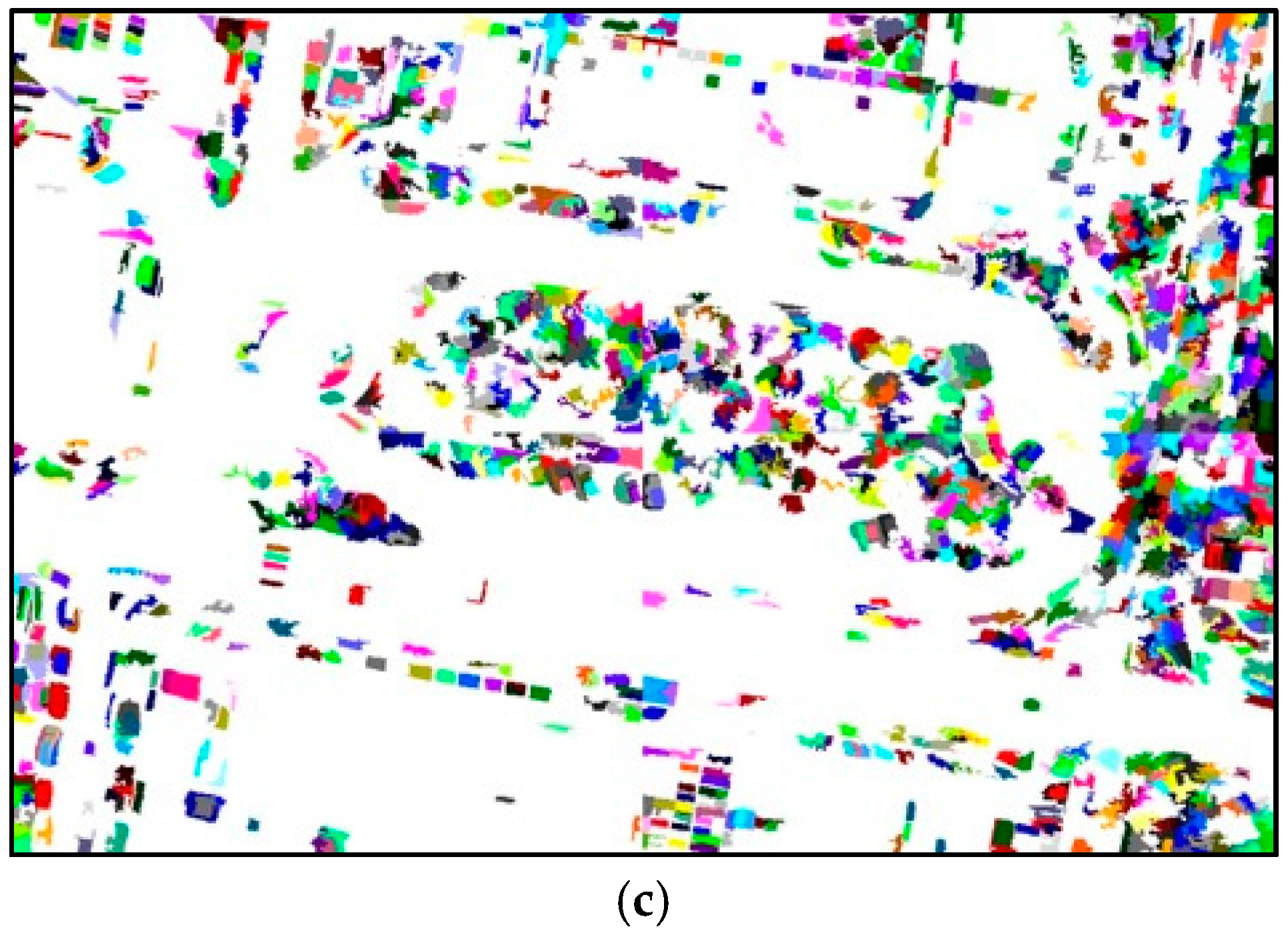
where ρ is a normalization parameter and h = [ h s , h r ] is the kernel bandwidth. Segmentation is essentially a merging process performed on a region that is produced by Mean-shift filtering. The use of the Mean-shift segmentation algorithm requires the selection of the bandwidth parameter h, which (by controlling the size of the kernel) determines the resolution of the mode detection. It can be noted that the Mean-shift algorithm cannot segment very large resolution images; however, we can divide the large image into smaller parts, apply the Mean-shift algorithm to each part separately, and combine the result (which is the method used to get the results in Figure 2b). Applying the Mean-shift algorithm in this way does not have any negative side effects on the final results.
Nevertheless, one advantage of the Mean-shift algorithm is that it provides an opportunity for the early elimination of large areas of the image based on the size of large regions. For example, as shown in Figure 2b, most of the asphalt regions (like roads and parking lots) are segmented in large regions, which can be easily removed from the search space automatically by including only regions that have a width or height close to the average car size in the image. By applying this simple technique, only the regions shown in Figure 2c needed to be included in the search space.

2.2. Feature Extraction with Pre-Trained CNNs

Deep CNNs are composed of several layers of processing—each containing linear as well as non-linear operators—which are jointly learnt in an end-to-end way to solve specific tasks [35,36]. Specifically, deep CNNs are commonly made up of convolutional, normalization, pooling, and fully connected layers. The convolutional layer is the main building block of the CNN, and its parameters consist of a set of learnable filters. Each filter is spatially small (along width and height), but extends through the full depth of the input image. The feature maps produced via convolving these filters across the input image are then fed into a non-linear gating function such as the rectified linear unit (ReLU) [37]. Next, the output of this activation function can be further subjected to normalization (i.e., local response normalization) to help in generalization.
The pooling layer takes small rectangular blocks from the convolutional layer and subsamples it to produce a single output from each block. The literature conveys several ways to perform pooling, such as taking the average, the maximum, or a learned linear combination of the values in the block. This layer allows control of over-fitting and reduces the amount of parameters and computation in the network.
After several convolutional and pooling layers, the high-level reasoning in the neural network is done via fully connected layers. A fully connected layer takes all neurons in the previous layer and connects it to every single neuron it has. In the case of classification, a softmax layer is added at the end of this network, where the number of neurons is equal to the number of classes. Finally, the weights of a CNN are learned using back-propagation techniques.
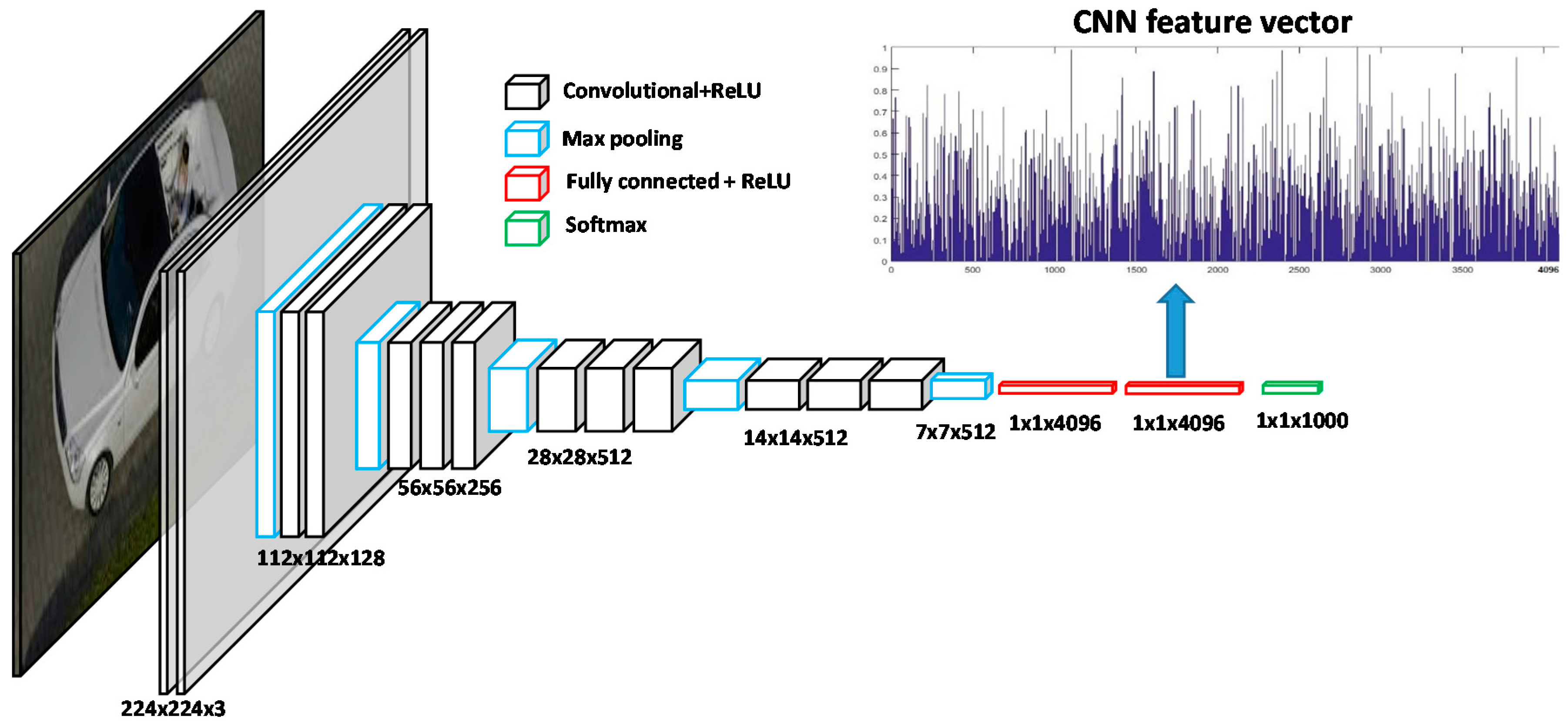
Usually, deep CNNs perform well with sufficient training data. However, they may lead to over-fitting problems for applications with limited training images. One possible solution is to transfer knowledge to CNNs (pre-trained on other domains) with very large sets of training images. Possible knowledge transfer solutions include fine-tuning the network on the new training images through back-propagation or feeding the images to pre-trained CNNs for feature generation. In the case of the latter, these extracted features can be used to train an external classifier (e.g., SVM). For the purpose of our study, we took the output of the hidden fully connected layer (before the softmax layer) of the VGG16 CNN as the feature descriptor for the training and test images (Figure 3).
The VGG16 CNN is a 16-layer network proposed by the VGG team in the ILSVRC 2014 competition [38]. This network is mainly composed of 13 convolutional layers, 5 pooling layers, and 3 fully connected layers. The network was trained on 1.2 million RGB images of 224 × 224 pixel size belonging to 1000 classes related to general images such as beaches, dogs, cats, cars, shopping carts, minivans, etc., and this auxiliary domain is completely different from the UAV datasets used in our experiments. The image regions identified by the Mean-shift algorithm were first resized to be of size 224 × 224 pixels, and they were then fed into the pre-trained CNN, yielding features of dimension 4096, as shown in Figure 3.

2.3. Region Classification with a Linear SVM

During this step, we went through all regions in the image and checked if they represented a car. To do this, we extracted a window surrounding the concerned region and passed it to a pre-trained CNN for feature extraction. Next, the feature descriptor was classified as either a “car” or “no-car” using an SVM classifier. This last step was trained on a collection of image samples for both classes. The set of positive samples was manually annotated in the training images, while the set of negative samples was randomly selected from the remaining areas of the training images.
The window surrounding the concerned region could be defined in two ways: (1) as the bounding box of the region, or (2) as a window centered at the centroid of the region with a given size. By inspecting the regions in Figure 4a, we could clearly see that for many small regions that represented parts of the car (like the roof or the front windshield), taking the bounding box may not have contained sufficient car features for high quality detection. The second option should yield better results.
Furthermore, cars in images can have any direction; thus, if rectangular windows are used, several window angles must be inspected. This significantly increases computational costs; however, in practice it was found that a square window of a reasonable size could capture features from a car in any direction sufficiently for successful detection. The size of this window must be neither too small nor too large: if the region is part of a car and the window size is too small, then not enough car features are captured and therefore miss detection. If the region is not part of car and the window size is too large, there is a risk of including parts of close-by cars and increasing false alarms. Thus, care should be taken to set this parameter to a suitable value, based on a sensitivity analysis experiment.

2.4. Fine-Tuning the Detection Result

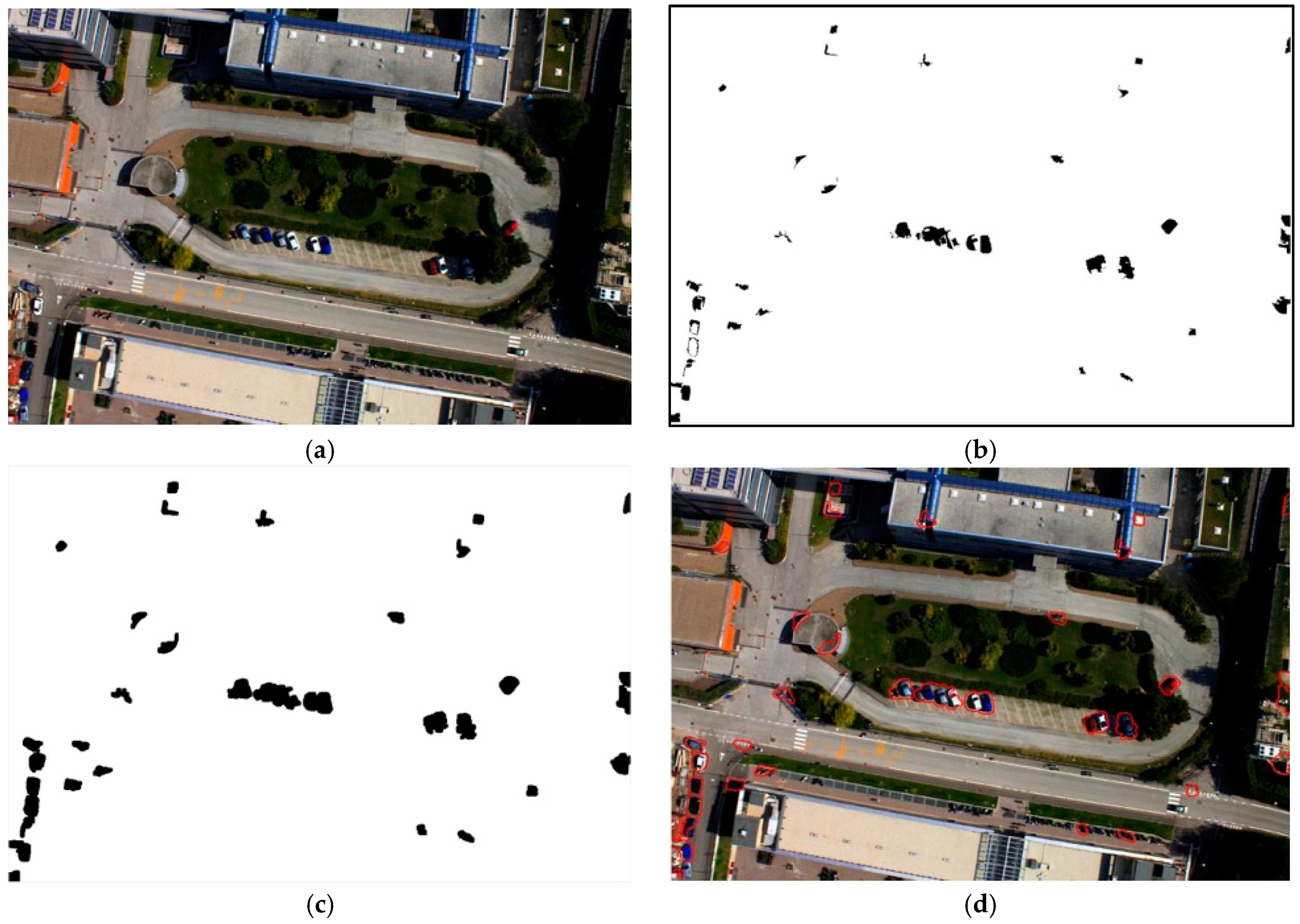
The result of Step 3 was a binary map showing all regions that were classified as car regions (Figure 5b). In this last fine-tuning step, we cleaned up the final map by applying three extra operations: (1) applying a morphological dilation operation on the detection map to smooth out region boundaries and merge close-by regions; (2) filling holes that may have appeared in detected regions; and (3) inspecting small isolated regions to improve the detection of isolated cars and potentially reduce false alarms.
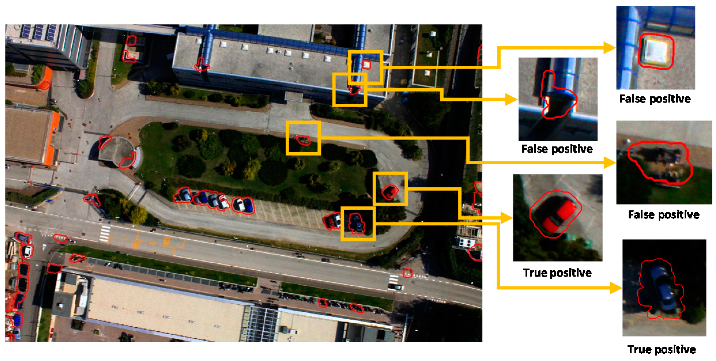
As observed in Figure 5d, the results show that the method achieved a high true positive (TP) rate; however, there was also a relatively high false positive (FP) rate. This was due to some small isolated regions of the image containing car-like signatures. First, it was noted that cars were usually parked in groups close to each other, and most regions detected as cars were next to each other. Hence, such regions merged into larger regions in the final mask, and only a few isolated regions remained spread across the image. Some examples of these small isolated regions are shown in Figure 6, where it is clear that some of them indicate a real parked car in an isolated area, and that there were many false positives. To remove some of these false positives, we propose some further analysis.
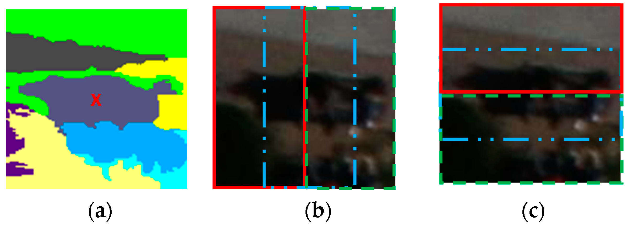
Our basic idea was to use small rectangular sliding windows around each of these isolated regions and pick the rectangular window that provided the highest detection score given by the SVM classifier. A total of six rectangular sliding windows were checked: three horizontal and three vertical (Figure 7), which used one of the wrongly detected regions shown in Figure 6 as an example. This example contained what looked like a motor bike parked in the street. As cars are rectangular in shape, using horizontal and vertical rectangular windows should further fine-tune the location of the car in isolated regions which do contain cars. For regions that do not contain a car (i.e., false positives), using such windows may break the car-like signature and remove the false positive.
Finally, to estimate the number of cars in an UAV image, we followed the approaches given in References [7,9], where the total area A of each detected region in the final map was divided by the average car size S a v g ; i.e., number of cars = round (A/ S a v g ). More details about the method of assessment are given in Section 3.1.

3. Results

3.1. Dataset Description and Experiment Setup

To evaluate the effectiveness of the proposed car detection method, we used a set of real images acquired by a UAV equipped with imaging sensors spanning the visible range. Nadir acquisitions were performed with a camera (Canon EOS 550D), characterized by a CMOS APS-C sensor with 18 megapixels. The images were acquired over the Faculty of Science, University of Trento, Trento, Italy, on 3 October 2011, at 12:00 p.m. The images were characterized by three channels (RGB) with 8 bits of radiometric resolution and a spatial resolution of 2 cm ground sample distance (GSD).
As per Reference [9], we used the same images as training and testing sets to be able to compare our results. A total of eight images were selected: three for training and five for testing. The training images are shown in Figure 8 with the car locations annotated with colored boxes.
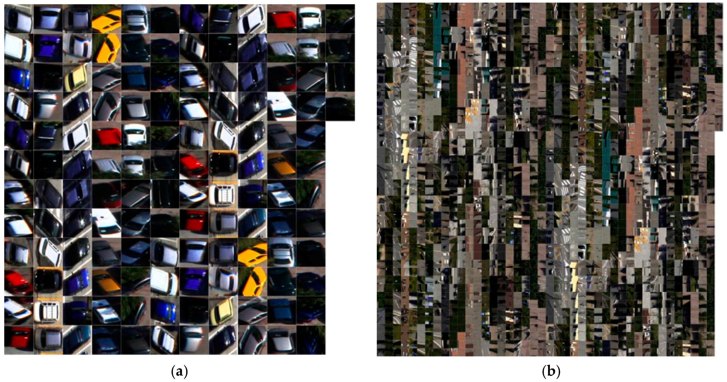
A total of 136 positive (car) training images (Figure 9a) were detected from these training images by including the annotated patches. In addition, 1864 negative (no-car) images (Figure 9b) were extracted from random locations in the remaining background areas. The size of the training patches was set to be equal to the average bounding boxes of the annotated cars. To increase the number of positive training images, we augmented the data by flipping the car images horizontally and vertically. This had the effect of multiplying the number of positive training images by three and allowed an increase in the generalization ability of the network.
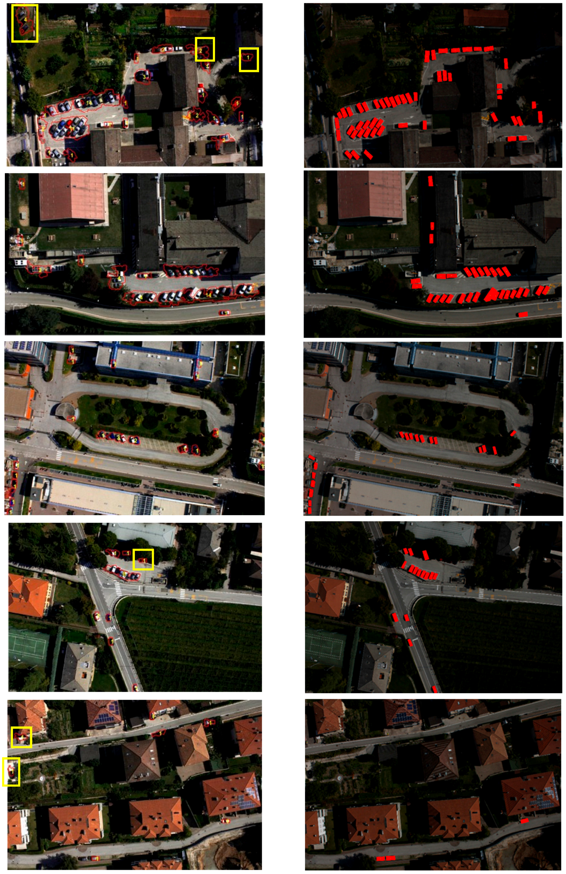
For testing purposes, five images (Figure 10) were used to test the robustness of the detection technique. Two images representing a large number of cars (Test Images 1 and 2) were of large parking lots with 56 and 31 cars, respectively; two images (Test Images 3 and 4) representing a medium number of cars were two standard urban areas with 19 and 16 cars, respectively; and Test Image 5 had only five cars to assess the method in the presence of a small number of isolated cars.
In Step 1, each test image was over-segmented into homogenous regions using the Mean-shift algorithm. The minimum region size used to run the Mean-shift algorithm was set to a tenth of the average car size. This was reasonable, given that we did not expect one car to be segmented to more than 10 regions. As the extracted regions have variable sizes, and given that the known average car appearing in our test images was approximately 200 × 90 pixels, there was no point in inspecting regions larger than 200 × 200 pixels. Therefore, all regions that had a bounding box whose width or length was greater than 200 were eliminated beforehand. For the remaining regions within the size limitations, a window with a size of 160 × 160 pixels was grabbed around each region (then normalized to 224 × 224 pixels) and fed to CNN for feature extraction. Step 2 of the algorithm was to classify each grabbed window using SVM with a linear kernel. The related regularization parameter C was estimate using a three-fold cross-validation technique within the range [10−3, 103].
The detection map was constructed by simply setting all pixels that belong to the regions that are classified as “car” to 1. All other pixels that belong to regions that are classified as “no-car” are set to 0. Obviously, the neighboring regions which are set to 1 will merge into one large region in the detection map. We then apply morphological dilation with a circular structure element of size 15 pixels. We found that using a larger size for the structure element increased the areas to points where it overestimated the final car count. Finally, a hole filling algorithm was applied, and each small isolated region was further inspected using rectangular sliding windows (as explained in Section 2.4).

3.2. Assessment Method

To assess the capability of our methodology for correct identification, we considered the accuracy measures of the producers and users, defined as follows:
P a c c = T P N
U a c c = T P T P + F P
where T P are the true positives (i.e., the number of cars correctly identified), F P are the false positives (i.e., the number of cars incorrectly identified), and N is the real number of cars present in the image. To compute these values, we needed a method to estimate the number of cars in the detection map. As mentioned previously, this was accomplished by dividing the total area of every detected region by the average car size:
N i = r o u n d ( A i S a v g ) ;   i :   1     R n
where R n is the total number of detected regions, A i is the area in pixels for each region, S a v g is the average car size, and N i is the estimated number of cars in that region. However, for small isolated cars, N i may be rounded to zero, in which case we simply set N i = N i + 1. As for the average car size in pixels S a v g , given that the UAV images at hand have a resolution of 2 cm GSD, then S a v g can be estimated as 200 × 90 pixels (which corresponds to an average real car size of 400 cm × 180 cm).
Finally, the F P i value for each region was computed as the difference between the number N i of detected cars in that region and the true number of cars present in the same region. The total FP for the whole image is computed as:
F P =   i = 1 R n F P i

3.3. Detection Results

Figure 10 shows the final detection map for all test images, as well as the estimated number of cars for each detection area, and Table 1 reports the quantitative detection results. We can also report that our method even detected cars that were hidden by shadows or partially occluded by buildings or trees that had not been initially included in the ground truth by human observers due to their high difficulty. These newly detected cars are highlighted by the yellow boxes in Figure 10. In particular, the extra cars that are present in the test images are as follows: five extra cars in Image 1, one extra car in Image 4, and two extra cars in Image 5. Thus, the new number of cars present in Images 1–5 are now 56, 31, 19, 16, and 5, respectively. The accuracy results shown in Table 1 were calculated based on the new number of cars present.

4. Discussions

4.1. Sensitivity Analysis with Respect to the Window Size

As previously mentioned, the size of the window fed to the pre-trained CNN must be carefully selected. In this section, we conducted an experiment to analyze the sensitivity of the detection results with respect to the window size. Table 2 presents the results of the sensitivity analysis for one test image using different window sizes. From the sensitivity analysis experiment, we concluded that a window size of 160 × 160 pixels (i.e., 80% of the average car size—200 × 200 pixels) provided the best total accuracy (93.6%).

4.2. Comparison with State-of-the-Art

Table 3 presents a comparison of our results to a recent method based on handcrafted features presented in Reference [9]. This is a method which aims at detecting cars and estimating their number under different conditions, including shadows, partial occlusions, and different orientations. First, note that we compared our method to the scenario in Reference [9] that did not include pre-screening of the image using GIS software to remove all non-asphalt regions (where cars are not expected to be present). For the set of scenarios that did not include pre-screening, we compared our results to the one based on the normalized cross-correlation similarity measure, as it produced the best result. Additionally, for a fair comparison, we did not include the extra cars that were detected by our method but were not included in the ground truth shared by Reference [9].
Our proposed method was not only superior in terms of detection accuracy, but was also much faster. The method in Reference [9] was reported to take an average of 3.9 h to process each test image, compared to the times shown in Table 3, which shows computational times between 11–30 min, depending on the complexity of image.

5. Conclusions

In our study, we developed an efficient method for the detection and counting of cars in UAV images, which has the following novel features: (1) reducing the search space significantly compared to the sliding-window approach by using the Mean-shift algorithm; and (2) the use of deep learning approaches to extract highly descriptive features without the need for huge amounts of training data through the use of pre-trained deep CNN combined with a linear SVM classifier. The experimental results on five UAV images show that our method outperformed state-of-the-art methods, both in terms of accuracy and computational time. However, despite the high capability of the method to detect car presence and numbers, it still has a high FP rate. Thus, future work is required to investigate ways to remove these false positives, perhaps through a “detection by parts” method or others. Another future direction is to investigate how to detect each car separately to increase accuracy in the car count.

Acknowledgments

The authors would like to extend their sincere appreciation to Deanship of Scientific Research at King Saud University for funding this Research group No. (RG-1435-050). The authors would like to thank Farid Melgani from University of Trento, Italy, for providing the images used in the experiments.

Author Contributions

Nassim Ammour, Haikel Alhichri and Yakoub Bazi developed the method and designed the experiments; Bilel Benjdira performed the experiments; Nassim Ammour, Haikel Alhichri, and Yakoub Bazi analyzed the results; Naif Alajlan and Mansour Zuair contributed the use of analysis tools; all authors contributed in writing and reviewing the manuscript. All authors read and approved the final manuscript.

Conflicts of Interest

The authors declare no conflict of interest.

References

  1. Colomina, I.; Molina, P. Unmanned aerial systems for photogrammetry and remote sensing: A review. ISPRS J. Photogramm. Remote Sens. 2014, 92, 79–97. [Google Scholar] [CrossRef]
  2. Berni, J.; Zarco-Tejada, P.J.; Suarez, L.; Fereres, E. Thermal and Narrowband Multispectral Remote Sensing for Vegetation Monitoring From an Unmanned Aerial Vehicle. IEEE Trans. Geosci. Remote Sens. 2009, 47, 722–738. [Google Scholar] [CrossRef]
  3. Uto, K.; Seki, H.; Saito, G.; Kosugi, Y. Characterization of Rice Paddies by a UAV-Mounted Miniature Hyperspectral Sensor System. IEEE J. Sel. Top. Appl. Earth Obs. Remote Sens. 2013, 6, 851–860. [Google Scholar] [CrossRef]
  4. Püschel, H.; Sauerbier, M.; Eisenbeiss, H. A 3D Model of Castle Landenberg (CH) from Combined Photogrammetric Processing of Terrestrial and UAV-based Images. Int. Arch. Photogramm. Remote Sens. Spat. Inf. Sci. 2008, 37, 93–98. [Google Scholar]
  5. Moranduzzo, T.; Mekhalfi, M.L.; Melgani, F. LBP-based multiclass classification method for UAV imagery. In Proceedings of the 2015 IEEE International Geoscience and Remote Sensing Symposium (IGARSS), Milan, Italy, 26–31 July 2015; pp. 2362–2365. [Google Scholar]
  6. Lin, A.Y.-M.; Novo, A.; Har-Noy, S.; Ricklin, N.D.; Stamatiou, K. Combining GeoEye-1 Satellite Remote Sensing, UAV Aerial Imaging, and Geophysical Surveys in Anomaly Detection Applied to Archaeology. IEEE J. Sel. Top. Appl. Earth Obs. Remote Sens. 2011, 4, 870–876. [Google Scholar] [CrossRef]
  7. Moranduzzo, T.; Melgani, F. A SIFT-SVM method for detecting cars in UAV images. In Proceedings of the 2012 IEEE International Geoscience and Remote Sensing Symposium, Munich, Germany, 22–27 July 2012; pp. 6868–6871. [Google Scholar]
  8. Moranduzzo, T.; Melgani, F. Automatic Car Counting Method for Unmanned Aerial Vehicle Images. IEEE Trans. Geosci. Remote Sens. 2014, 52, 1635–1647. [Google Scholar] [CrossRef]
  9. Moranduzzo, T.; Melgani, F. Detecting Cars in UAV Images With a Catalog-Based Approach. IEEE Trans. Geosci. Remote Sens. 2014, 52, 6356–6367. [Google Scholar] [CrossRef]
  10. Moranduzzo, T.; Melgani, F.; Bazi, Y.; Alajlan, N. A fast object detector based on high-order gradients and Gaussian process regression for UAV images. Int. J. Remote Sens. 2015, 36, 37–41. [Google Scholar]
  11. Zhao, T.; Nevatia, R. Car detection in low resolution aerial image. In Proceedings of the Eighth IEEE International Conference on Computer Vision (ICCV 2001), Washington, WA, USA, 7–14 July 2001. [Google Scholar]
  12. Moon, H.; Chellappa, R.; Rosenfeld, A. Performance analysis of a simple vehicle detection algorithm. Image Vis. Comput. 2002, 20, 1–13. [Google Scholar] [CrossRef]
  13. Kluckner, S.; Pacher, G.; Grabner, H.; Bischof, H.; Bauer, J. A 3D Teacher for Car Detection in Aerial Images. In Proceedings of the 2007 IEEE 11th International Conference on Computer Vision, Rio de Janeiro, Brazil, 14–21 October 2007; pp. 1–8. [Google Scholar]
  14. Holt, A.C.; Seto, E.Y.W.; Rivard, T.; Gong, P. Object-based Detection and Classification of Vehicles from Highresolution Aerial Photography. Photogrammetric Engineering and Remote. Photogramm. Eng. Remote Sens. 2009, 75, 871–880. [Google Scholar] [CrossRef]
  15. Shao, W.; Yang, W.; Liu, G.; Liu, J. Car detection from high-resolution aerial imagery using multiple features. In Proceedings of the 2012 IEEE International Geoscience and Remote Sensing Symposium, Munich, Germany, 22–27 July 2012; pp. 4379–4382. [Google Scholar]
  16. Chen, X.; Xiang, S.; Liu, C.-L.; Pan, C.-H. Vehicle Detection in Satellite Images by Hybrid Deep Convolutional Neural Networks. IEEE Geosci. Remote Sens. Lett. 2014, 11, 1797–1801. [Google Scholar] [CrossRef]
  17. Leitloff, J.; Rosenbaum, D.; Kurz, F.; Meynberg, O.; Reinartz, P. An Operational System for Estimating Road Traffic Information from Aerial Images. Remote Sens. 2014, 6, 11315–11341. [Google Scholar] [CrossRef]
  18. Xu, Y.; Yu, G.; Wang, Y.; Wu, X.; Ma, Y. A Hybrid Vehicle Detection Method Based on Viola-Jones and HOG + SVM from UAV Images. Sensors 2016, 16, 1325. [Google Scholar] [CrossRef] [PubMed]
  19. Hinton, G.; Osindero, S.; Teh, Y. A Fast Learning Algorithm for Deep Belief Nets. Neural Comput. 2006, 18, 1527–1554. [Google Scholar] [CrossRef] [PubMed]
  20. Vincent, P.; Larochelle, H.; Bengio, Y.; Manzagol, P.-A. Extracting and Composing Robust Features with Denoising Autoencoders. In Proceedings of the 25th International Conference on Machine Learning, Helsinki, Finland, 5–9 July 2008; ACM: New York, NY, USA, 2008; pp. 1096–1103. [Google Scholar]
  21. Swietojanski, P.; Ghoshal, A.; Renals, S. Convolutional Neural Networks for Distant Speech Recognition. IEEE Signal Process. Lett. 2014, 21, 1120–1124. [Google Scholar]
  22. Lampert, C.H.; Blaschko, M.B.; Hofmann, T. Beyond sliding windows: Object localization by efficient subwindow search. In Proceedings of the 2008 IEEE Conference on Computer Vision and Pattern Recognition, Anchorage, AK, USA, 23–28 June 2008; pp. 1–8. [Google Scholar]
  23. Vedaldi, A.; Gulshan, V.; Varma, M.; Zisserman, A. Multiple kernels for object detection. In Proceedings of the 2009 IEEE 12th International Conference on Computer Vision, Kyoto, Japan, 27 September–4 October 2009; Volume 1, pp. 606–613. [Google Scholar]
  24. Girshick, R.; Donahue, J.; Darrell, T.; Malik, J. Rich feature hierarchies for accurate object detection and semantic segmentation. In Proceedings of the IEEE Computer Society Conference on Computer Vision and Pattern Recognition, Columbus, OH, USA, 24–27 June 2014; pp. 580–587. [Google Scholar]
  25. Wang, X.; Yang, M.; Zhu, S.; Lin, Y. Regionlets for Generic Object Detection. IEEE Trans. Pattern Anal. Mach. Intell. 2015, 37, 2071–2084. [Google Scholar] [CrossRef] [PubMed]
  26. Uijlings, J.R.R.; Van De Sande, K.E.A.; Gevers, T.; Smeulders, A.W.M. Selective Search for Object Recognition. Int. J. Comput. Vis. 2013, 104, 154–171. [Google Scholar] [CrossRef]
  27. Ren, S.; He, K.; Girshick, R.; Sun, J. Faster R-CNN: Towards Real-Time Object Detection with Region Proposal Networks. IEEE Trans. Pattern Anal. Mach. Intell. 2016. [Google Scholar] [CrossRef] [PubMed]
  28. Cheng, Y. Mean shift, mode seeking, and clustering. IEEE Trans. Pattern Anal. Mach. Intell. 1995, 17, 790–799. [Google Scholar] [CrossRef]
  29. Comaniciu, D.; Meer, P. Mean shift: A robust approach toward feature space analysis. IEEE Trans. Pattern Anal. Mach. Intell. 2002, 24, 603–619. [Google Scholar] [CrossRef]
  30. Boykov, Y.; Funka-Lea, G. Graph Cuts and Efficient N-D Image Segmentation. Int. J. Comput. Vis. 2006, 70, 109–131. [Google Scholar] [CrossRef]
  31. Jianbo Shi, J.; Malik, J. Normalized cuts and image segmentation. IEEE Trans. Pattern Anal. Mach. Intell. 2000, 22, 888–905. [Google Scholar] [CrossRef]
  32. Vedaldi, A.; Soatto, S. Quick Shift and Kernel Methods for Mode Seeking. In Computer Vision—ECCV 2008; Forsyth, D., Torr, P., Zisserman, A., Eds.; Springer: Berlin/Heidelberg, Germany, 2008; Volume 5305, pp. 705–718. [Google Scholar]
  33. Vincent, L.; Soille, P. Watersheds in digital spaces: An efficient algorithm based on immersion simulations. IEEE Trans. Pattern Anal. Mach. Intell. 1991, 13, 583–598. [Google Scholar] [CrossRef]
  34. Levinshtein, A.; Stere, A.; Kutulakos, K.N.; Fleet, D.J.; Dickinson, S.J.; Siddiqi, K. TurboPixels: Fast superpixels using geometric flows. IEEE Trans. Pattern Anal. Mach. Intell. 2009, 31, 2290–2297. [Google Scholar] [CrossRef] [PubMed]
  35. Farabet, C.; Couprie, C.; Najman, L.; Le Cun, Y. Learning Hierarchical Features for Scene Labeling. IEEE Trans. Pattern Anal. Mach. Intell. 2013, 35, 1915–1929. [Google Scholar] [CrossRef] [PubMed]
  36. Brosch, T.; Tam, R. Efficient Training of Convolutional Deep Belief Networks in the Frequency Domain for Application to High-resolution 2D and 3D Images. Neural Comput. 2015, 27, 211–227. [Google Scholar] [CrossRef] [PubMed]
  37. Krizhevsky, A.; Sutskever, I.; Hinton, G.E. Imagenet classification with deep convolutional neural networks. In Advances in Neural Information Processing Systems; MIT Press: Cambridge, MA, USA, 2012. [Google Scholar]
  38. Simonyan, K.; Zisserman, A. Very Deep Convolutional Networks for Large-Scale Image Recognition. In Proceedings of the 3rd International Conference on Learning Representations, San Diego, CA, USA, 7–9 May 2015. [Google Scholar]
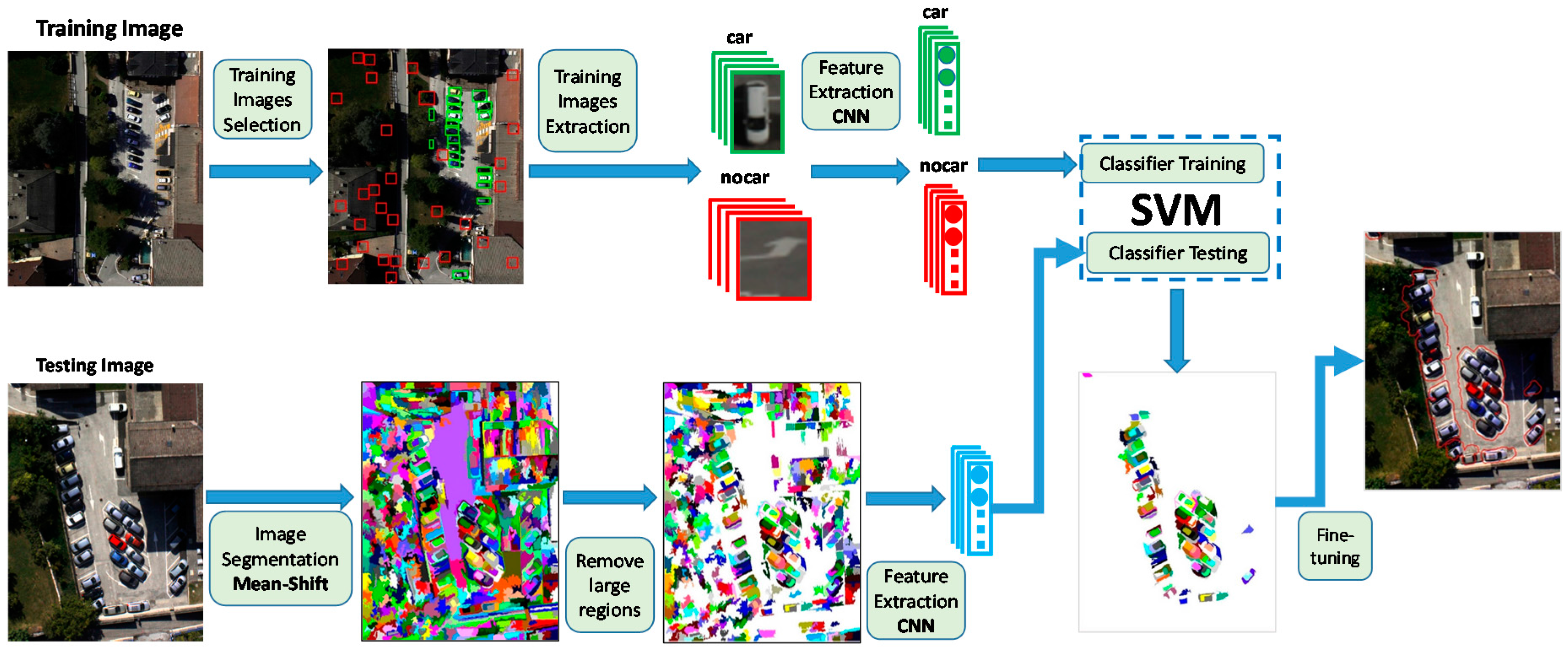
Figure 1. Flowchart of the proposed car counting method. CNN: convolutional neural network; SVM: support vector machine.
Remotesensing 09 00312 g001
Figure 2. (a) Original image; (b) Mean-shift algorithm result with parameters hr = 1, hs = 2, with a minimum region size of 50 pixels; and (c) Regions obtained after the filtering step.
Remotesensing 09 00312 g002aRemotesensing 09 00312 g002b
Figure 3. Overview of the architecture of the VGG-16 pre-trained CNN and its use for feature extraction. ReLU: rectified linear unit.
Remotesensing 09 00312 g003
Figure 4. A small region can be any part of a car, like the roof or the windshield. (a) Examples of true positives; and (b) examples of false positives.
Remotesensing 09 00312 g004
Figure 5. Detection results of Test Image 3. (a) Original image; (b) positively classified regions; (c) detection mask results after morphological operation; and (d) detection mask superimposed on image.
Remotesensing 09 00312 g005
Figure 6. Samples of small isolated regions where some are isolated parked cars (true positive) while others are false positives.
Remotesensing 09 00312 g006
Figure 7. Six rectangular sliding windows were further inspected for each small isolated window. (a) The small isolated positive region; (b) vertical sliding windows; and (c) horizontal sliding windows.
Remotesensing 09 00312 g007
Figure 8. Training images (ac) with a total of 136 cars annotated. Training patches for the “no car” class were selected randomly from the remaining background.
Remotesensing 09 00312 g008
Figure 9. Training samples images collected: (a) 136 car samples; and (b) 1863 no car samples.
Remotesensing 09 00312 g009
Figure 10. Detection results of the proposed algorithm for Test Images 1–5 together with their ground truths. Particularly difficult cars that were detected by the proposed algorithm are highlighted with yellow boxes.
Remotesensing 09 00312 g010
Table 1. Detection results for the test images. FP: false positive; TP: true positive.
Test ImageSizeRegionsWithin RangeCars PresentTPFPPaccUaccAcc
Image 12626 × 4680466640065647483.9%92.2%88.0%
Image 22424 × 38963114248331261083.9%72.2%78.0%
Image 33456 × 5184462312821914773.7%66.7%70.2%
Image 43456 × 5184647321651613081.3%100.0%90.6%
Image 53456 × 51846666199454280.0%66.7%73.3%
Table 2. Example of sensitivity analysis with respect to the window size parameter for Test Image 2.
Window Size in Pixels% of Average Car SizeTPFPPaccUaccAccCars Present
60 × 6030%18260.0%90.0%75.0%30
80 × 8040%24180.0%96.0%88.0%30
100 × 10050%25183.3%96.2%89.7%30
120 × 12060%26386.7%89.7%88.2%30
140 × 14070%27390.0%90.0%90.0%30
160 × 16080%29396.7%90.6%93.6%30
180 × 18090%26586.7%83.9%85.3%30
200 × 200100%27890.0%77.1%83.6%30
Table 3. Comparison to state-of-the art methods.
Proposed MethodMethod in [9]
Test ImageSizeCars PresentTPFPAccTime (s)Cars PresentTPFPAcc
Image 12626 × 46805143487.9%159251351073.2%
Image 22424 × 389631261078.0%81531201560.8%
Image 33456 × 51841914770.2%41619163059.5%
Image 43456 × 51841512090.0%72615141769.2%
Image 53456 × 518432258.3%657323935.8%
Total1199723 11987111