Detection of Flavescence dorée Grapevine Disease Using Unmanned Aerial Vehicle (UAV) Multispectral Imagery

Abstract

Flavescence dorée is a grapevine disease affecting European vineyards which has severe economic consequences and containing its spread is therefore considered as a major challenge for viticulture. Flavescence dorée is subject to mandatory pest control including removal of the infected vines and, in this context, automatic detection of Flavescence dorée symptomatic vines by unmanned aerial vehicle (UAV) remote sensing could constitute a key diagnosis instrument for growers. The objective of this paper is to evaluate the feasibility of discriminating the Flavescence dorée symptoms in red and white cultivars from healthy vine vegetation using UAV multispectral imagery. Exhaustive ground truth data and UAV multispectral imagery (visible and near-infrared domain) have been acquired in September 2015 over four selected vineyards in Southwest France. Spectral signatures of healthy and symptomatic plants were studied with a set of 20 variables computed from the UAV images (spectral bands, vegetation indices and biophysical parameters) using univariate and multivariate classification approaches. Best results were achieved with red cultivars (both using univariate and multivariate approaches). For white cultivars, results were not satisfactory either for the univariate or the multivariate. Nevertheless, external accuracy assessment show that despite problems of Flavescence dorée and healthy pixel misclassification, an operational Flavescence dorée mapping technique using UAV-based imagery can still be proposed.

1. Introduction

Flavescence dorée (FD) is a serious phytoplasma-borne disease widespread in many European countries [1]. The FD disease is transmitted from between grapevines in the field by the leafhopper Scaphoideus titanus Ball. (Hemiptera: Cicadellidae) [2,3] which is native to North America and was introduced in Europe in the late 1950s [4]. This leafhopper feeds and reproduces almost exclusively on grapevines (Vitis vinifera L., Vitaceae) and is the only known vector of FD. The main symptoms of the disease appear in late summer and remain visible until mid-autumn when: (a) the canes droop because of a lack of lignification in the new shoots; (b) the leaves become yellowish in white cultivars or reddish in red ones (discoloration intensity is variable and may affect the entire grapevine, only one shoot, or a small number of shoots) and (c) drying of the inflorescence and berries occurs [5]. Finally, the infected plants generally stop producing grapes and often die after a few years. Another phytoplasma grapevine disease, called Bois noir, may show similar symptoms and the diagnostic is based on specific molecular analysis. Given the epidemic potential of the disease and the severe damage caused in major vine- and wine- producing European countries, FD is a quarantined disease in the European and Mediterranean Plant Protection Organization (EPPO) region (Directive 77/1993 amended 92/103). Therefore, FD is subject to the following mandatory control procedures: (a) use of healthy plant material; (b) spray of insecticides against the vector; and (c) uprooting of the infected plants to remove sources of FD phytoplasma [1,6]. In France, when a vineyard plot has more than 20% of the vines infected by the FD disease, the entire plot must be removed. Despite all of these prophylactic procedures, FD is still spreading in Europe and is considered, with grapevine trunk diseases, as one of the most economically important disease of the European grapevine in its principal wine-production areas [1,7]. Among the main costs for growers, the removal of FD-infected grapevines constitutes a substantial cost. In most French vineyard regions, despite considerable efforts, the final area surveyed to detect infected plants is insufficient to eradicate all sources of FD phytoplasma. Vineyard surveys are usually made by foot (or using quad vehicle) and can result in mechanical damage and, as symptoms are not easy to detect, FD can be confused with other diseases or plant deficiences [8].

Remote sensing (RS) data has been frequently cited as a rapid, non-destructive, and cost-effective tool for plant disease detection in different contexts and with different plant species [9,10,11,12]. Indeed, several diseases can affect plant physiology, leading to modifications on biophysical and biochemical characteristics of tissues and differences in leaf optical properties [13,14,15,16]. RS techniques adopted in the plant disease literature are often based on well known, or specifically designed, vegetation indices (VI) that are tested and calibrated as indicators for the detection a given disease [12,14,15,17,18,19,20,21,22]. In these studies, the potential of hyperspectral imagery is often highlighted, but several difficulties are associated with this kind of data (financial costs, amount of data, specific processing tasks).

Grapevine disease detection remains a challenging topic. Ideally, the spatial resolution should be adapted to detect even a single infected plant over an entire vineyard plot. In addition, sensor bands must cover the useful portions of the electromagnetic spectrum in order to discriminate healthy from infected plants and, sometimes, to be able to detect different intensities of the disease. The efficiency of RS data to detect foliar symptoms has already be studied of other grapevine diseases like Phylloxera [17], Leaf roll virus [23], Plasmopora viticola [24] or Esca [12]. Because of the structural characteristics of vineyards, these studies often use high and very high spatial resolution images, with pixel dimensions ranging from a few meters (with satellite imagery) to a few centimeters (with unmanned aerial vehicle (UAV) imagery). UAV imagery is particularly adapted for vineyard monitoring owing to its very high spatial resolution (often below 10 cm) and flexible mission planning [25,26]. UAV imagery is of great interest for FD detection as the symptoms are often distributed in small patches and might only be visible during short periods in a year.

Given the importance of the FD disease in French and European vineyards, several research projects related to different aspects of the disease are currently underway. However, to the best of our knowledge, the potential of UAV remotely-sensed data to detect the Flavescence dorée symptoms has not yet been assessed.

This paper evaluates the potential to detect FD grapevine disease using UAV multispectral imagery by testing the capacity of three types of UAV-derived variables (spectral bands, vegetation indices and biophysical parameters) to detect FD symptoms in red and white cultivars.

The rest of the paper is organized as follows: Section 2 presents the data acquisition, processing and analysis. Section 3 describes and discusses the main experimental results obtained with univariate and multivariate classification approaches. Conclusions and perspectives are drawn in Section 4.

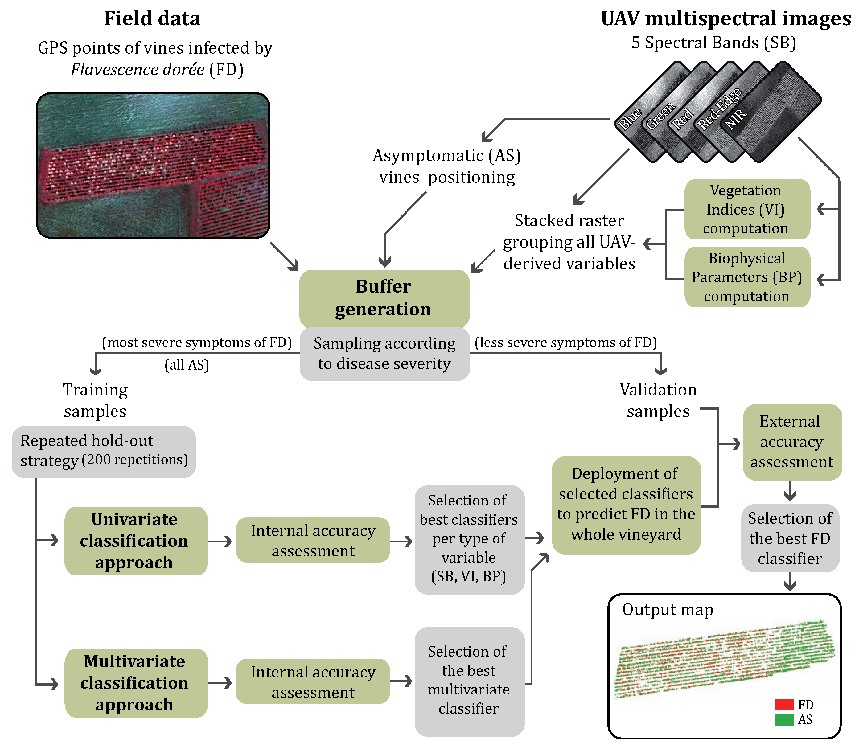
2. Materials and Methods

2.1. Data Acquisition

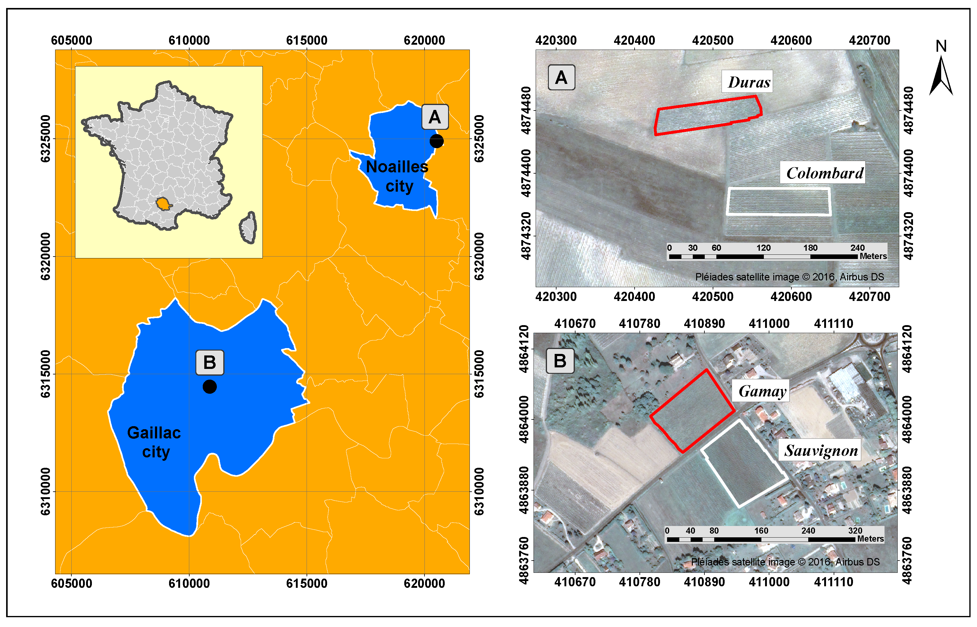
2.1.1. Experimental Sites

The research was conducted in the Gaillac Appellation d’Origine Contrôlée (AOC) area in Southwest France. Four vineyards infected by FD disease were selected over two different sites A and B (see Figure 1). They are not irrigated and usually contain inter-row herbaceous vegetation. Vine and row spacing are around 1 m and 2 m, respectively. Two vineyards consisted of white cultivars, Sauvignon and Colombard, and the other two vineyards featured red cultivars, Gamay and Duras. Red cultivars were more severely infected by the FD disease than the white ones.

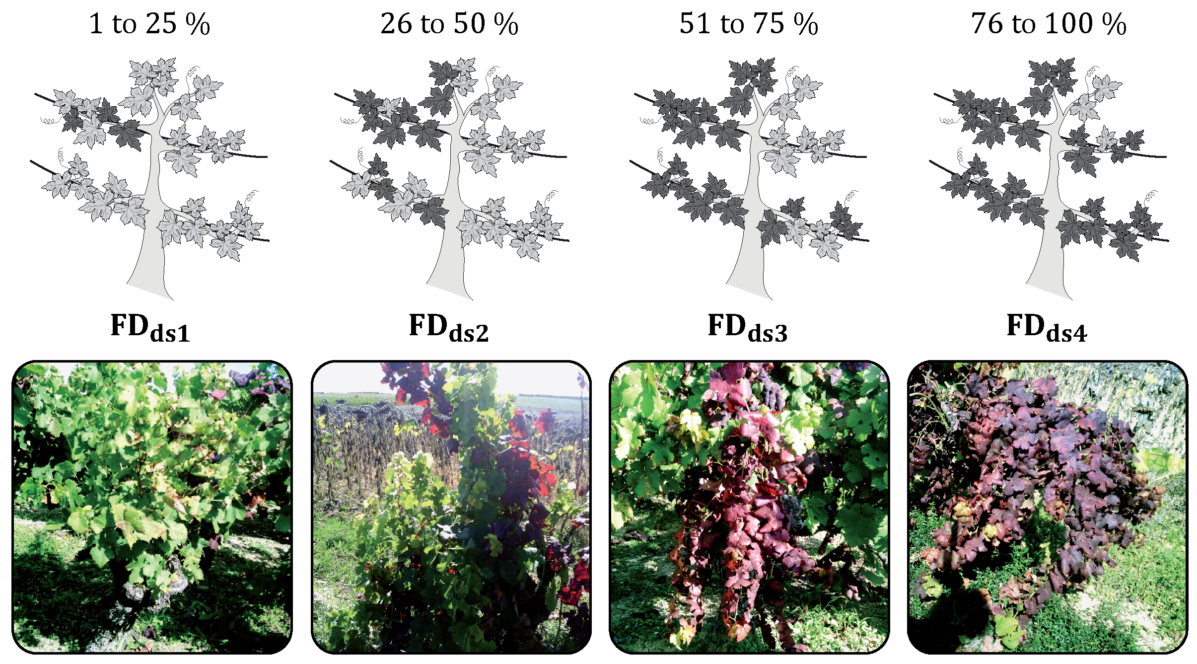
2.1.2. Field Data Acquisition

Concurrent field and UAV flight campaigns were conducted in September 2015 when the FD symptoms were fully expressed. This time corresponded to the final stage of maturation of the berries (i.e., a few days before fruit harvesting).

Field data acquisition consisted of collecting the precise location of all the vines presenting FD symptoms in the four vineyards. This task was performed with a portable differential Global Positionning System - GPS (Trimble Geo7X) providing highly accurate positioning (horizontal precision of 0.02 m). For each GPS point, Flavescence dorée disease severity (FD_ds) was recorded. According to [27], disease severity is the area (relative or absolute) of the sampling unit (leaf, fruit, etc.) showing symptoms of disease and is often expressed as a percentage or proportion. In this work, the sampling unit is the vine and the disease severity corresponds to the percentage of the vine presenting visual symptoms of the FD disease during the field campaign. More in detail, Flavescence dorée disease severity (FD_ds), was reported as one of the four categories (FD_ds1, FD_ds2, FD_ds3, FD_ds4) as illustrated in Figure 2.

In addition to FD_ds, plant length (along the row) and width (perpendicular to the row) were measured for all the GPS points in the less affected vineyards (Sauvignon and Colombard) and for each 15 GPS points in the most affected vineyards (Gamay and Duras).

Table 1. Field data characteristics for the four selected vineyards (Gamay, Sauvignon, Duras and Colombard) in the Gaillac Appellation d’Origine Contrôlée (AOC) area during September 2015.

	Gamay	Sauvignon	Duras	Colombard
Berry color	red	white	red	white
Vineyard size (ha)	1.1	1.2	0.4	0.4
Row orientation	45.0°	135.0°	80.0°	100.0°
Number of positioned vines	389	9	264	40
Mean plant length (m)	1.34	1.40	1.15	1.68
Mean plant width (m)	0.48	0.92	1.02	0.84
Number of FDds1 (1% to 25%)	170	0	68	1
Number of FDds2 (26% to 50%)	103	7	44	3
Number of FDds3 (51% to 75%)	45	2	44	7
Number of FDds4 (76% to 100%)	71	0	108	29

summarizes the main characteristics of the data collected during the field campaign in the four vineyards.

2.1.3. UAV Multispectral Imagery Acquisition and Pre-Processing

The flight campaign was conducted by the Delair’Tech company on 21 September 2015 using a UAV platform (long range DT-18) able to fly by remote control or autonomously with the help of an integrated GPS receiver and a navigation system. UAV multispectral images were acquired with a DT-5Bands imaging instrument, based on the industry-leading MicaSense RedEdge^TM sensor. This sensor (see detailed description in

Table 2. UAV platform and sensor characteristics.

Characteristic Name	Description
Platform	Long range DT-18
Sensor	DT-5Bands
Sensor type	Global shutter—distortion free
Number of bands	5
Spectral wavelengths	Blue (455–495 nm)
	Green (540–580 nm)
	Red (658–678 nm)
	Red-Edge (707–727 nm)
	NIR (800–880 nm)
Dimension	3.6 mm × 4.8 mm
Automatic Gain Control	Yes
Resolution	960 × 1280 pixels
Focal length	5.5 mm
Field of view	47.2°
Output data	12-bit RAW
Image size	1.8 MB
Flight altitude Above Ground Level (AGL)	120 m
Image acquisition	5 images (each band)
Image triggering	Controlled by the autopilot
Ground resolution	0.08 m/pixel
Ground Picture Size	Width 105 m × Height 79 m at 120 m AGL
Surface area covered	3 ${\mathrm{km}}^2$ at 150 m AGL
Onboard storage	32 GB micro Secure Digital (SD) card
Calibrated panel	Included (with reflectance data)

) includes five independent high precision sensors to capture the vegetation response at five spectral bands (SB): blue, green, red, red-edge and near infrared (NIR). UAV flights were realized under clear sky conditions and with optimal illumination conditions in both sites (local time in Central European Summer Time–CEST): between 12:25 and 14:13 for the Duras and Colombard vineyards and between 14:17 and 14:59 for the Gamay and Sauvignon vineyards. Flight altitude was set at 120 m with a UAV flight speed of 6 m/s. These specific settings enabled an 85% image forward overlap and a 70% image side overlap for optimal photogrammetric processing.

Pix4D software (Available at: https://pix4d.com/) was used to manage and process the UAV images. Images covering the two sites were orthorectified (using a 0.08-m resolution digital elevation model), grouped into a mosaic, projected in World Geodetic System (WGS) 84/Universal Transfer Mercator (UTM) zone 31N coordinate system, and re-sampled at 0.10-m ground spatial resolution (see Figure 3). Pixel values were converted to surface reflectance in each spectral band, thanks to the calibrated ground panel used before and after the flight (to check stability of the illumination). The output product delivered for each site was a unique stacked raster file (GeoTiff format) containing five spectral bands.

2.2. Data Processing and Analysis

Field data and UAV imagery were conjointly processed in order to detect the symptoms of the Flavescence dorée in the four vineyards. Figure 4 shows the main steps of the methodological framework developed in this research. These steps are described in the following sub-sections.

2.2.1. Computing Vegetation Indices and Biophysical Parameters

A set of eleven vegetation indices (VI) and four biophysical parameters (BP) were calculated from the five spectral bands (SB) of the UAV images. These were chosen because of their potential relevance to discriminate symptomatic and asymptomatic vines infected by the Flavescence dorée disease.

Table 3. Summary of selected vegetation indices.

Index Name	Formula	References
Normalized difference vegetation index	$NDVI={\displaystyle \frac{NIR-Red}{NIR+Red}}$	[41]
Anthocyanin reflectance index	$ARI=Gree{n}^{-1}-RedEdg{e}^{-1}$	[28,42]
Modified anthocyanin reflectance index	$MARI=(Gree{n}^{-1}-RedEdg{e}^{-1})\times NIR$	[28,42,43]
Red-green index	$RGI={\displaystyle \frac{Red}{Green}}$	[28,44]
Anthocyanin content index	$ACI={\displaystyle \frac{Green}{NIR}}$	[45]
Modified anthocyanin content index	$MACI={\displaystyle \frac{NIR}{Green}}$	[28]
Chlorophyll index	$CI={\displaystyle \frac{NIR}{RedEdge}}-1$	[29,43]
Green-red vegetation index	$GRVI={\displaystyle \frac{Green-Red}{Green+Red}}$	[46,47]
Soil-adjusted vegetation index	$SAVI={\displaystyle \frac{(NIR-Red)\times (1+L)}{NIR+Red+L}}$	[48]
Green normalized difference vegetation index	$GNDVI={\displaystyle \frac{NIR-Green}{NIR+Green}}$	[49]
Difference vegetation index	$DVI=NIR-Red$	[50,51]

gives formulas and corresponding references for the vegetation indices selected. The selected VI were used for monitoring and mapping temporal and spatial variations of biomass and plant productivity (NDVI, SAVI, GNDVI) and for estimating the leaf pigments (ARI, MARI, RGI, ACI, MACI, CI, GRVI). Among them, NDVI have been already used to detect ESCA disease in vineyard [12]; Steele and Gitelson studied RGI, ARI, MARI for their potential to estimate anthocyanin [28] and CI for chlorophyll content in grapevine leaves [29]. Most of these VI are band ratios and so are robust to variation of the sun illumination (which was not significant here anyhow, thanks to the clear sky conditions). Biophysical parameters were generated using the Overland software for biophysical processing developed by Airbus DS Geo-Intelligence. The Overland tool was initially developed in order to retrieve vegetation parameters (leaf area index, LAI, chlorophyll, fCover) from satellite images, the produced maps serving as inputs to recommendation products towards the end-users (crop growers). It has been extensively tested and validated in this context [30]. In France, the Farmstar service is operational since 2002 and 80,000 crop fields subscribed to this service in 2016. The advantage of BP is that, unlike most VI, they do not depend on variables such as geometry of illumination or sensor characteristics. They are then often considered as very good candidates to replace classical vegetation indices for characterizing and monitoring green vegetation [31,32,33,34]. The parameters exploited here are presented in

Table 4. Summary of selected biophysical parameters.

Parameter Name	Acronym	Description	Unit and Typical Range
fCover	fCov	Fractional cover of green vegetation	0.0 to 1.0
		(interception in vertical view)
Leaf Chlorophyll content	Chl	Chlorophyll content in the leaves	20 to 80 $\mathsf{\mu }\mathrm{g}/\mathrm{c}{\mathrm{m}}^2$
		(per leaf unit area)
Leaf Anthocyanin content	Ant	Anthocyanin content in the leaves	0 to 12 $\mathsf{\mu }\mathrm{g}/\mathrm{c}{\mathrm{m}}^2$
		(per leaf unit area)
Leaf Carotenoid content	Car	Carotenoid content of the leaves	0 to 15 $\mathsf{\mu }\mathrm{g}/\mathrm{c}{\mathrm{m}}^2$
		(per leaf unit area)

. The Overland tool extracts vegetation parameters by inverting a canopy reflectance model [35] that is based on the coupling of the PROSPECT leaf model and the scattering by arbitrary inclined leaves (SAIL) canopy model [36]. PROSPECT is a physical model simulating directional–hemispherical reflectance and transmittance of leaves based on a set of biochemical constituents and a structure parameter [37]. The initial version of PROSPECT included chlorophyll and equivalent water thickness (EWT) as the only input parameters related to leaf chemical constituents. Several versions of the model have been developed to include a larger variety of input parameters related to leaf chemical constituents and properties, such as leaf mass per area (LMA). In terms of pigment content, two versions have been released to allow for separating the influence of different types of pigments on leaf optical properties. PROSPECT-5 [38] allowed separating the influence of chlorophyll and carotenoids on leaf optical properties. PROSPECT-D is the latest version of the model, and it allows separating the influence of chlorophyll, carotenoids and anthocyanins, along with EWT and LMA [39]. Therefore PROSPECT-D is able to simulate optical properties during the lifespan of the leaf and for a new range of conditions, including broadened juvenile and senescent stages, as well as environmental stresses induced by temperature, pollution and plant pathogens, which impact leaf pigment composition.

SAIL (scattering by arbitrary inclined leaves) [40] simulates the bidirectional reflectance factor of plant canopies, describing vegetation as a turbid medium characterized by leaf optical properties and structural properties such as leaf area index (LAI) and leaf angular distribution function (LADF). It also takes into account the spectral characteristics of the soil underneath vegetation, as well as the geometry of acquisition (sun and viewing directions). Various versions have been developed in order to add complexity to the original simplistic description of vegetation. This includes a combination of SAIL with geometrical models in order to describe horizontally and vertically heterogeneous vegetation, introduction of crown clumping, and hot spot effects. The coupled PROSPECT+SAIL model, called PROSAIL, inputs simulated leaf reflectance and transmittance from the PROSPECT model into the SAIL model to simulate the whole canopy reflectance [36]. For the specific case of UAV images, various modifications were made to the initial model. In particular, it can adapt to different cases of UAV acquisition conditions, including acquisitions made under a variable cloud cover (in which case cloud optical thickness is an actual variable of the model).

2.2.2. Buffer Generation and Sampling Strategy

Two processing steps were performed to extract FD pixels from UAV imagery. First, a site-specific mask was computed based on the output of a supervised classification. Supervised classification was performed with the support vector machine (SVM) algorithm [52], using a radial basis function (RBF) kernel. Four classes were used for training the SVM classifier: 1-bare soil, 2-shadow, 3-inter-row vegetation and 4-grapevine vegetation. Very high classification accuracy was achieved for the four vineyards (mean overall accuracy equalled 0.97 for the Gamay and Sauvignon and 0.99 for Duras and Colombard; mean values obtained from 100 repetitions using 10-fold cross-validation). Then, site-specific classification outputs were used to mask all UAV pixels except those classified as grapevine vegetation (hereafter called valid pixels). The second step consisted of generating a buffered area around each GPS point. A first buffer, named average buffer was computed as a rectangle taking into account row orientation and the mean values of length and width per vineyard (as shown in Table 1).

At this point, the dataset was composed of a collection of pixels extracted from the buffered areas (see methodological framework on Figure 4). Each pixel included 20 numerical variables (5 SB, 11 VI and 4 BP) and a categorical variable representing the disease severity observed in the field (FD_ds1, FD_ds2, FD_ds3 or FD_ds4).

Next, the collection of pixels for each vineyard was divided into two parts: (a) training samples and (b) validation samples. Training samples should be as pure as possible in order to avoid training a classifier with doubtful data. For this reason, FD vines showing the most severe symptoms were chosen as training samples for each vineyard. In addition, a second buffer, named reduced buffer, was computed for those vines (using the minimum values of plant width and length per vineyard). These precautions limited the number of mixed pixels within the training samples. In practice, a subset of the FD_ds4 vines presenting the most severe symptoms was selected. Due to the absence of FD_ds4 vines in the Sauvignon vineyard, FD_ds3 and FD_ds2 were instead used as training samples.

Table 5. Training and validation samples in each vineyard. The number of valid pixels is indicated between brackets.

		Gamay		Sauvignon		Duras		Colombard
		Train.	Val.	Train.	Val.	Train.	Val.	Train.	Val.
FDds1	number of vines	0	170	0	-	0	68	0	1
	(valid pixels)	(0)	(6243)	(0)	-	(0)	(5940)	(0)	(136)
FDds2	number of vines	0	103	7	-	0	44	0	3
	(valid pixels)	(0)	(3960)	(53)	-	(0)	(3867)	(0)	(354)
FDds3	number of vines	0	45	2	-	0	44	0	7
	(valid pixels)	(0)	(1709)	(14)	-	(0)	(4094)	(0)	(711)
FDds4	number of vines	24	47	0	-	58	50	21	8
	(valid pixels)	(287)	(1914)	(0)	-	(698)	(3987)	(244)	(762)
All FD	number of vines	24	367	9	-	58	206	21	19
	(valid pixels)	(287)	(13,826)	(67)	-	(698)	(17,888)	(244)	(1963)
AS	number of vines	24	-	9	-	58	-	21	-
	(valid pixels)	(293)	-	(77)	-	(676)	-	(260)	-

shows the amount of vines and valid pixels used as training or validation samples in each vineyard.

Finally, the training set was completed with asymptomatic vines (AS) identified by computer-assisted photointerpretation on UAV images. AS vines corresponded to plants not showing FD symptoms in the field and that were apparently healthy on UAV images. In order to provide a well-balanced training set, the same number of AS vines as FD vines (training) were selected per vineyard (see Table 5). The same procedure for computing the reduced buffer and extracting pixel values (SB, VI and BP) was applied to AS vines.

All the remaining FD vines were used as validation samples (pixels values extracted considering the average buffer per vineyard). Due to very low numbers of FD vines, no validation samples were selected for the Sauvignon vineyard.

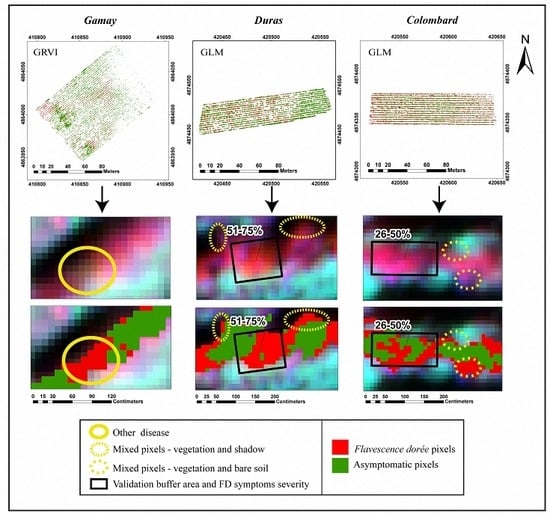
2.2.3. Detection of Flavescence dorée Symptoms on UAV Images

The objective here was to evaluate the reliability of Flavescence dorée disease detection using the variables derived from UAV images (SB, VI and BP) across the four selected vineyards. To this end, ArcMap (Version 10.2.2) and RStudio (Version 0.99.896 ) software were employed.

2.2.4. General Principle

Receiver operator characteristic (ROC) analysis was used to determine the capacity of each variable to discriminate FD or AS pixels. ROC curves have become a useful and well-studied tool for the evaluation of classifiers using remote sensing data [53].

The construction of a ROC curve, as applied to the detection of FD and AS at the pixel level, was considered a binary classification problem resulting from the thresholding of a variable (or classifier output). Here, a decision had to be made between two classes: FD or AS. Based on the data collected during the field campaign, four classification outcomes are possible (see

Table 6. Interpretation of potential classification outcomes.

		Reference Data
		Flavescence dorée (FD)	Asymptomatic (AS)
Classification	Flavescence dorée (FD)	True Positive	False Positive
		(FD pixel classified as FD)	(AS pixel classified as FD)
results	Asymptomatic (AS)	False Negative	True Negative
		(FD pixel classified as AS)	(AS pixel classified as AS)

).

Two indicators of classification performance, $sensitivity$ (or true positive rate) and $specificity$ (or true negative rate), are calculated based on Equations (1) and (2) respectively. These indicators are used to build the ROC curve with $sensitivity$ plotted as a function of $1-specificity$.

$$Sensitivity=TruePositive/(TruePositive+FalseNegative)$$

(1)

$$Specificity=TrueNegative/(TrueNegative+FalsePositive)$$

(2)

While testing a variable, the ROC curve is obtained by computing, for all possible threshold values (in a given interval and step), the corresponding values of $specificity$ and $sensitivity$. The optimal threshold corresponds to the point in the ROC curve where the sum of sensitivity and specificity is maximized. Based on the ROC curve, the area under the curve (AUC) is the metric used to assess the overall performance of the classifier. AUC ranges from 0.0 to 1.0, where the larger is the AUC, the higher are the $specificity$ and $sensitivity$ values. An ideal classifier corresponds to an AUC equal to 1.0 (no classification errors) whereas the AUC of a random classifier is equal to 0.5 (high number of errors).

2.2.5. Univariate and Multivariate Classification Approaches

In order to obtain more realistic estimates, all experiments were performed using a random repeated hold-out strategy (see internal accuracy assessment step in Figure 4). The number of repetitions was set to 200. For each run, 80% of the training samples were used for training the classifier and the remaining 20% for testing the accuracy. For both univariate and multivariate approaches, the experiments were carried out separately in each vineyard (Gamay, Sauvignon, Duras and Colombard).

A first ROC analysis, called ‘univariate’, was realized on each variable derived from the UAV images. The capacity of a given variable to discriminate FD or AS pixels was tested considering the optimal threshold computed from the ROC curve. According to AUC results, the best variables in each category (i.e., SB, VI and BP) were selected.

In parallel, another ROC analysis, called ‘multivariate’, was performed. Instead of analyzing separately each variable, we examined the binary response (FD or AS) of combined models. These models were constructed as generalized linear models (GLM) and the Akaike information criterion (AIC) was the metric used to evaluate their performance. AIC summarizes the trade-off between model accuracy and complexity [54,55]. Low AIC values for a model indicate a superior explanatory power. The GLM construction was coupled with a feature selection procedure. Starting from the full model (containing all the 20 UAV-derived variables), a backward elimination feature selection was performed to return the best GLM considering the AIC metric. As with the ‘univariate’ approach, a ROC analysis was applied to select the GLM optimal threshold and to estimate the classification performance in terms of $sensibility$, $specificity$, and AUC.

Each vineyard was then assigned a set of best classifiers selected via the internal accuracy assessment. Finally, these selected classifiers were trained with the whole training samples and deployed over the corresponding vineyards to predict the class (FD or AS) of the entire collection of valid pixels.

2.2.6. External Accuracy Assessment

External accuracy assessment was realized using the validation samples available for each vineyard (as shown in Table 5). Unlike training samples, validation samples were not related to pure patches of FD pixels. Instead, their buffered areas were composed of a rate of FD pixels with respect to AS pixels. As a consequence, the external accuracy assessment consisted of comparing rates of FD pixels (predicted by the selected classifiers) against the FD disease severity (FD_ds) observed in the field.

In order to get comparable information between field FD_ds and classifier-predicted FD rate, rates were first converted into four discrete classes (1, 2, 3 or 4), each corresponding to one of the four FD_ds classes. Considering that those classes are ordinal and equidistant, the external accuracy assessment was handled as a regression problem. The overall agreement between field and predicted classes for a given vineyard was verified through the root-mean-squared error (RMSE) as formalized in Equation (3). RMSE values of 1 or 3 respectively mean a difference of 1 or 3 FD_ds classes between field and predicted classes.

$$\mathrm{RMSE}=\sqrt{\frac{\sum {\left(ClassValu{e}_{\mathrm{predicted}}-ClassValu{e}_{\mathrm{field}}\right)}^2}{n}}$$

(3)

Even if the RMSE is a good metric to evaluate (punctually) the quality of the predictions and compare the performances of the classifiers, the number of validations samples was limited in most of the vineyards. Because of this, the external accuracy assessment was completed by a detailed visual analysis of the FD maps generated by the best classifier of each vineyard.

3. Results

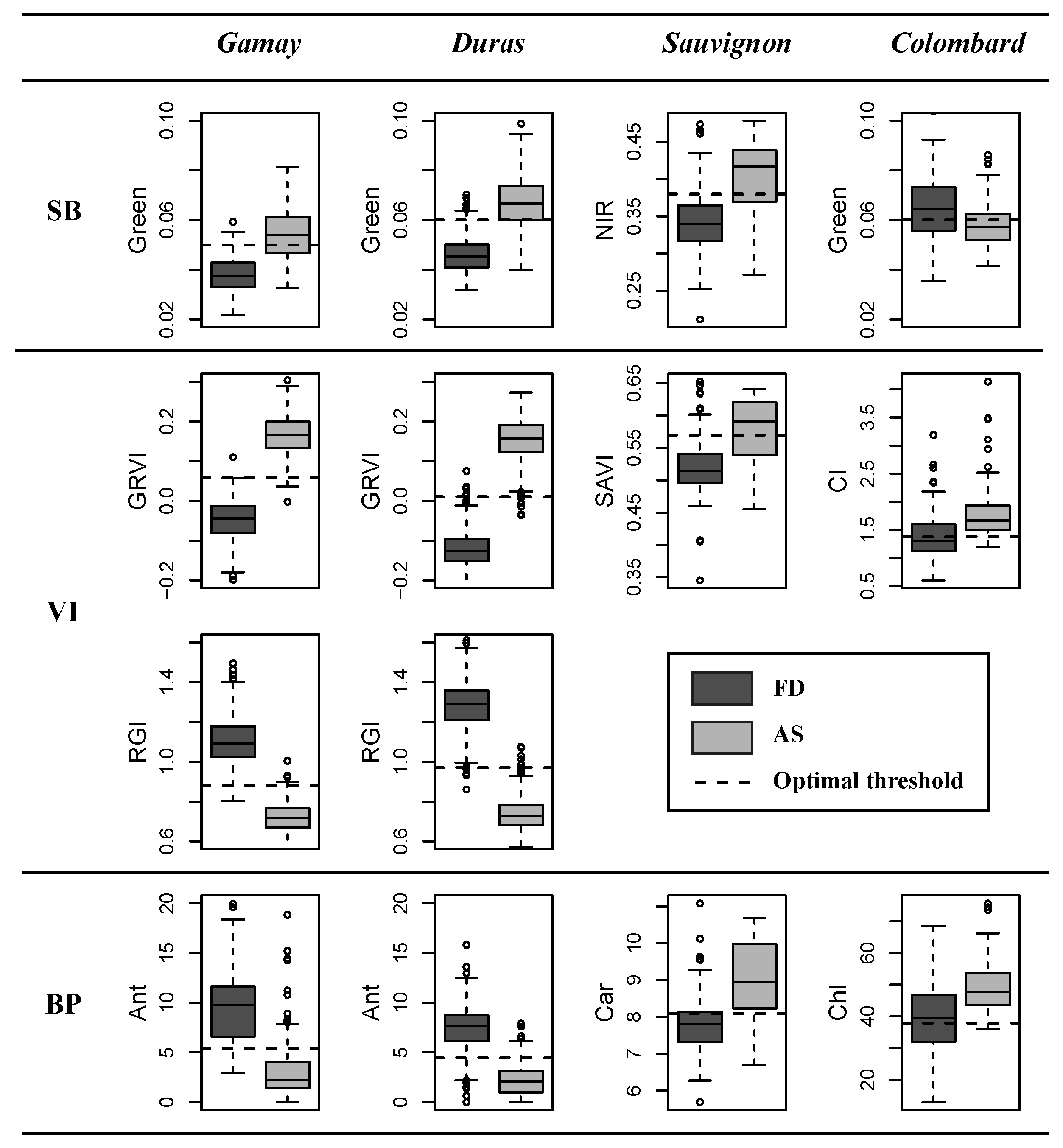
3.1. Univariate Accuracy Assessment

Table 7. Univariate accuracy assessment for each vineyard and cultivar. Mean area under the curve (AUC) and standard deviation (Std) was computed using a repeated holdout strategy (200 repetitions).

		Red Cultivars				White Cultivars
		Gamay		Duras		Sauvignon		Colombard
		Mean AUC	Std	Mean AUC	Std	Mean AUC	Std	Mean AUC	Std
SB	Blue	0.68	0.01	0.59	0.01	0.53	0.03	0.52	0.01
	Green	0.91	0.01	0.96	0.00	0.67	0.03	0.68	0.01
	Red	0.65	0.01	0.82	0.01	0.50	0.03	0.50	0.01
	RedEdge	0.70	0.01	0.52	0.01	0.66	0.02	0.63	0.01
	NIR	0.54	0.01	0.66	0.01	0.76	0.02	0.63	0.01
VI	NDVI	0.63	0.01	0.88	0.00	0.66	0.03	0.58	0.01
	ARI	0.94	0.00	0.98	0.00	0.64	0.02	0.67	0.01
	MARI	0.97	0.00	0.96	0.00	0.50	0.03	0.72	0.01
	RGI	1.00	0.00	1.00	0.00	0.75	0.02	0.76	0.01
	MACI	0.95	0.00	0.94	0.00	0.54	0.03	0.75	0.01
	ACI	0.95	0.00	0.94	0.00	0.53	0.02	0.75	0.01
	CI	0.71	0.01	0.75	0.01	0.64	0.02	0.78	0.01
	GRVI	1.00	0.00	1.00	0.00	0.75	0.02	0.76	0.01
	SAVI	0.50	0.01	0.76	0.01	0.76	0.02	0.63	0.01
	GNDVI	0.95	0.00	0.94	0.00	0.53	0.02	0.75	0.01
	DVI	0.52	0.01	0.71	0.01	0.76	0.02	0.63	0.01
BP	fCov	0.79	0.01	0.92	0.00	0.62	0.03	0.64	0.01
	Ant	0.94	0.00	0.97	0.00	0.65	0.02	0.55	0.01
	Car	0.81	0.01	0.85	0.01	0.80	0.02	0.49	0.01
	Chl	0.58	0.01	0.55	0.01	0.54	0.03	0.76	0.01

shows the mean AUC and standard deviation obtained from the ROC curves of the 20 variables studied (SB, VI and BP) for red (Gamay and Duras) and white (Sauvignon and Colombard) cultivars vineyards. For the two red cultivars vineyards, the best variables in each category are the same (Green for SB; GRVI and RGI for VI; Ant for BP). However, the best variables differ for the vineyards with the two white cultivars (Green or Red for SB; SAVI, DVI or CI for VI; Chl or Car for BP).

To characterize the performance of the best classifiers identified,

Table 8. Mean values of $sensitivity$ and $specificity$ for the best variables.

		Red Cultivars				White Cultivars
		Gamay		Duras		Sauvignon		Colombard
		Sens.	Spec.	Sens.	Spec.	Sens.	Spec.	Sens.	Spec.
SB	Green	0.89	0.74	0.94	0.85	-	-	0.46	0.81
	NIR	-	-	-	-	0.78	0.71	-	-
VI	RGI	1.00	0.98	0.99	0.99	-	-	-	-
	CI	-	-	-	-	-	-	0.58	0.89
	GRVI	0.99	0.98	0.99	0.99	-	-	-	-
	SAVI	-	-	-	-	0.81	0.67	-	-
	DVI	-	-	-	-	0.80	0.68	-	-
BP	Ant	0.88	0.82	0.90	0.92	-	-	-	-
	Car	-	-	-	-	0.72	0.74	-	-
	Chl	-	-	-	-	-	-	0.50	0.92

presents the specificity (Spec.) and sensitivity (Sens.) also computed from the ROC curves. Next, results are analyzed for each category of variables.

3.1.1. Spectral Bands

Given the three categories of variables, SB had the lowest power to discriminate between FD and AS pixels regardless of cultivar. Among the five available SBs, the Green band was the best classifier for the two red cultivars and the Colombard white cultivar while the NIR band was best for the Sauvignon white cultivar. For these two SB, mean AUC values and associated sensitivity and specificity were higher for the red cultivars than for the white. This was especially true for Colombard which had an AUC 0.68 and sensitivity of 0.46, suggesting poor performance of the Green band. However, in both cases, misclassification of FD and AS pixels remained. For example, using the Green band for Duras resulted in the highest AUC and values for sensitivity and specificity of 0.94 and 0.85, respectively. Despite this, it was estimated that 6% of true FD and 15% of true AS pixels would be misclassified.

3.1.2. Vegetation Indices

For red and white cultivars, VI performed better than SB to discriminate FD and AS pixels. For the two red cultivars, RGI and GRVI—both derived from the green and red bands—were the two best classifiers. The mean AUC was equal to 1 and the sensitivity and specificity were equal or superior to 0.98 indicating a very high power of separability of FD and AS pixels. Classification performance was poorer for the two white cultivars. The best mean AUC was obtained with different VI and differed with the cultivar. For Sauvignon, it was the SAVI and DVI with an AUC of 0.76. For Colombard, it was the CI with an AUC of 0.78. In both cases, sensitivity and specificity did not reach satisfying values. The amount of true FD pixels misclassified as AS pixels (1.00-$Sensitivity$) ranged between 19% and 42%. The amount of true AS pixels misclassified as FD pixels (1.00-$Specificity$) varied between 11% and 33%.

3.1.3. Biophysical Parameters

BP performed better than SB but worse than VI for all cultivars. For the two red cultivars, very good results were obtained with Ant (close to the one obtained with GRVI and RGI), especially for Duras with a mean AUC of 0.97 and associated sensitivity and specificity of 0.90 and 0.92 respectively. For the two white cultivars, results similar to those seen with the VI were observed. The best mean AUC were obtained with different BP according to the cultivar (Car with an AUC of 0.80 for Sauvignon; Chl with an AUC of 0.76 for Colombard). Values of sensitivity and specificity indicated that classifying FD and AS pixels with these BP still resulted in high levels of error. For example, the amount of pixels misclassified as AS pixels (1.00-Sensitivity) was estimated between 28% and 50%.

To sum up, Figure 5 presents the box plots of the FD and AS pixels with the best classifier per vineyard (in column) and per category of variable (in row). The optimal threshold values calculated with all training data is symbolized with a black dashed line. For variables with an AUC equal or close to 1 (RGI and GRVI for Duras and Gamay), a low covering up between FD and AS pixels was observed indicating their very high potential of FD discrimination. For variables with an AUC lower than 0.8 (all variables selected for white cultivars), the confusion between FD and AS pixels was clearly visible meaning a potentially high level of misclassification. Finally, interval and distribution of values of variables were not homogeneous according the type of cultivar (red or white). As a consequence, even if the same best classifier (GRVI) was found for the red cultivars, the optimal threshold value was specific for each vineyard (0.06 for Gamay and 0.01 for Duras).

3.2. Multivariate Accuracy Assessment

3.2.1. Features Selection

Table 9. Multivariate accuracy assessment per vineyard. Mean and standard deviation computed from repeated holdout strategy (200 repetitions). AIC: Akaike information criterion.

		Red Cultivars		White Cultivars
		Gamay	Duras	Sauvignon	Colombard
Full model	Mean AIC	38	81	113	334
	Num. of variables	20	20	20	20
Simplified model	Mean AIC	20	61	101	326
	Num. of variables	9	7	10	12
	Gain (% AIC reduction)	47	26	11	2
Simplified model AUC	Mean	1.00	1.00	0.95	0.95
	Std	0.00	0.00	0.01	0.01
Simplified model sensitivity	Mean	0.99	0.99	0.80	0.82
	Std	0.01	0.01	0.11	0.06
Simplified model specificity	Mean	0.97	0.99	0.85	0.90
	Std	0.02	0.01	0.11	0.06

presents the results of the backward elimination method used for each vineyard to select the most interesting of the 20 initial variables for use in the GLM to discriminate FD and AS pixels. Compared to the full model, all simplified models reduced the AIC between 2% and 47% indicating a systematic improvement of the power of explanation. The number of variables was significantly reduced and differed according to the vineyard, ranging between 9 for Gamay and 12 for Colombard.

Table 10. Selected variables per vineyard with the backward elimination method.

Type of Model	Cultivar	List of variables
Full model	(all)	[Blue + Green + RedEdge + NIR + NDVI + ARI + RGI + MACI + ACI
		+ CI + GRVI + SAVI + GNDVI + DVI + GLCV + Ant + Car + Chl]
Simplified models	Gamay	[Blue + NDVI + AVI + GNDVI + MACI + ACI + CI + GRVI + Car]
	Sauvignon	[Green + RedEdge + NIR + NDVI + RGI + ACI + GRVI + DVI + fCov + Car]
	Duras	[Blue + NIR + RGI + GRVI + DVI + Chl + Car]
	Colombard	[RedEdge + NIR + NDVI + ARI + RGI + ACI + MACI + CI + GRVI + SAVI + GNDVI + Chl]

describes the simplified GLMs for each vineyard. First, GRVI was always present in the simplified models regardless of cultivar. This confirmed what was previously observed in the ‘univariate’ analysis—a high potential for this VI to discriminate FD and AS pixels. Second, for red cultivars, the BP Car and the Blue band were in both models. The same result was observed for the white cultivars. Two SB (Red Edge and NIR) and four VI (GRVI, NDVI, RGI and ACI) were retained in the simplified GLM. Except for the NIR, in the case of the Sauvignon vineyard, none of these variables for red and white cultivars were found to be the best classifier in the ‘univariate’ analysis.

3.2.2. GLM Performance Assessment

The ROC analysis is applied on the simplified GLMs. Table 9 shows mean and standard deviation for AUC, sensitivity and specificity for each vineyard. The performance of the ‘multivariate’ approach was assessed by comparing these values with ones obtained from the ‘univariate’ analyses. Mean AUC values were equal to 1 for red cultivars with associated sensitivity and specificity of 0.99 suggesting a high-performing model. Nevertheless, the quality of FD and AS discrimination was the same across the ‘univariate’ and ‘multivariate’ classification approaches. For the white cultivars, however, the three metrics were significantly better with the ‘multivariate’ approach. The mean AUC value of 0.95 observed for both Sauvignon and Colombard represents a 20% increase compared to mean AUCs obtained from the best classifiers for these cultivars in the ‘univariate’ analysis. Even with improved sensitivity and specificity, these values indicate remaining FD and AS misclassification. Finally, the best classifier was provided by the GLM for three vineyards (Duras, Sauvignon and Colombard). For Gamay, GRVI and RGI perform slightly better than the GLM but differences were not significant.

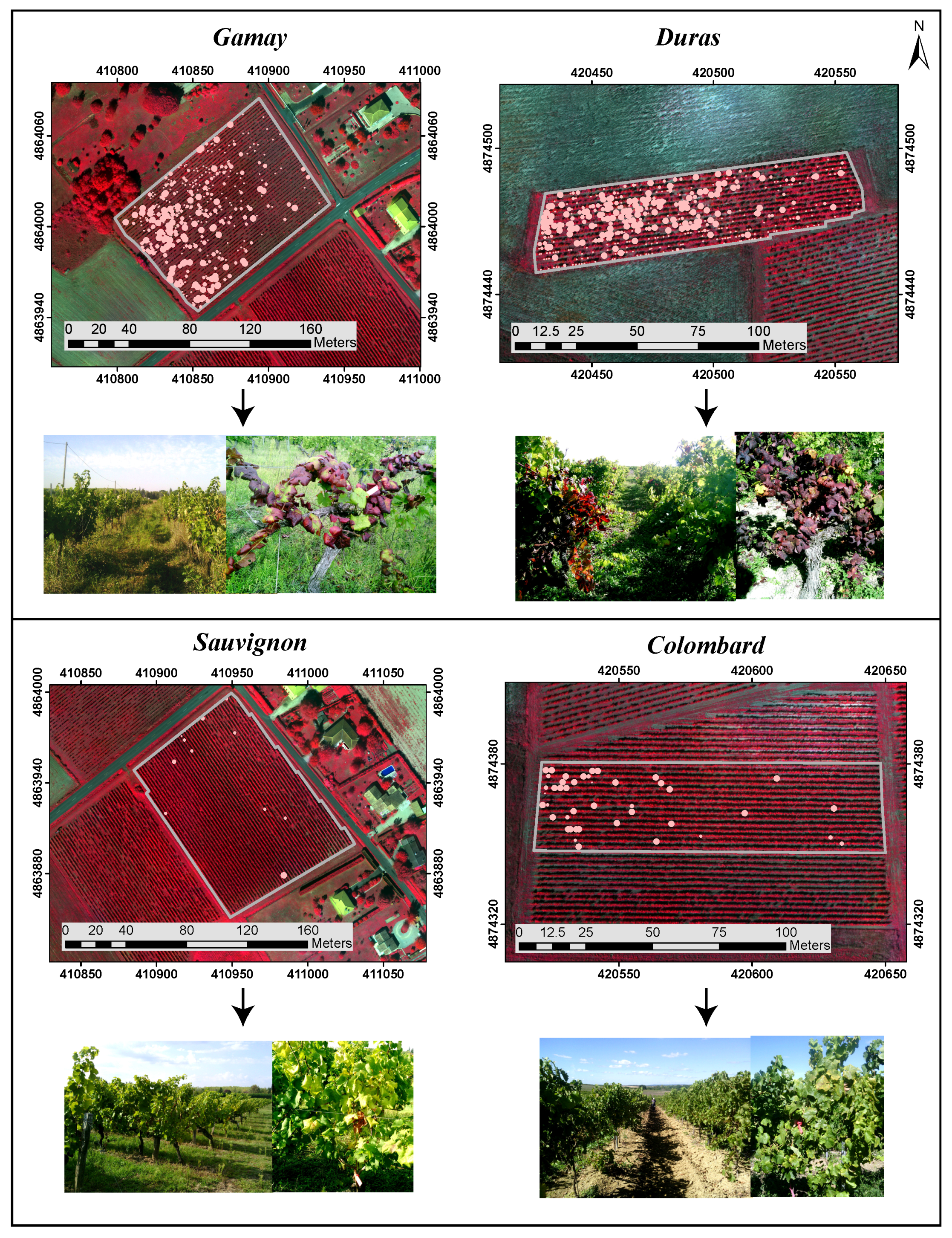
3.3. Application to Whole Vineyards and External Accuracy Assessment

Table 11. Validation results per vineyard (external accuracy assessment). RMSE: root-mean-square error. n: number of validation sample.

	Gamay		Duras		Colombard
Ranked Position	Classifier	RMSE (n = 365)	Classifier	RMSE (n = 206)	Classifier	RMSE (n = 19)
1	GRVI	1.24	GLM	1.16	GLM	1.28
2	RGI	1.24	GRVI	1.21	CI	1.76
3	GLM	1.27	RGI	1.21	Green	1.99
4	Green	1.38	Green	1.25	Chl	2.28
5	Ant	1.50	Ant	1.26

presents, for the three vineyards for which validation data were available, the results of the comparison between the rates of FD pixels predicted by the selected classifiers against the FD disease severity FD_ds observed in the field. In general, for the two red and one white cultivars, the RMSE indicated a difference of one FD_ds class. For the red cultivars, the GLM classifier performed equally well to the best classifiers found in the ‘univariate’ analysis (with a RMSE between 1.16 and 1.27). For the Colombard cultivar, the GLM classifier was significantly better (GLM RMSE of 1.28 vs. other classifiers RMSE between 1.76 and 2.28).

The external accuracy assessment step was completed by visually analyzing the FD maps realized with the best classifiers. Figure 6 presents for each vineyard (in column) a general overview of the classification result for all pixels labeled as ’grapevine vegetation’ (first row) and three subsets illustrating the main situations causing misclassification of true FD and AS pixels (second row). From these maps, two major observations were made. First, true FD areas were effectively predicted as FD for the three vineyards. Second, overestimation of FD pixels existed in all cases but was more obvious for white than red cultivars. In this study, the problem of false FD pixels can be explained by: (1) confusion with other diseases symptoms as illustrated in Figure 6 (second row—left); (2) confusion with AS mixed pixels containing either grapevine vegetation and shadow (Figure 6, second row—center) or vegetation and bare soil (Figure 6, second row—right).

4. Discussion

4.1. Univariate and Multivariate Analyses

From the ‘univariate’ analysis, we observed first that, regardless of the category, classifying FD and AS pixels with one variable yielded better results for red cultivar vineyards. Moreover, for all the best classifiers, sensitivity and specificity estimates obtained with the optimal threshold show that confusion between FD and AS pixels was less important for red than white cultivars though present in both cases. This is not surprising as leaves reddening on red cultivars was actually much more visible in field than leaves yellowing on white cultivars (Figure 3). Consequently, FD symptoms on white cultivars were characterized by a spectral response closer to AS pixels compared to red cultivars as shown in Figure 5. We also showed that, of the three variable categories, VI had generally the best power of discrimination between FD and AS pixels for red and white cultivars even if, in some cases, SB or BP might also be of value. For red cultivars, the best classifiers obtained were based on either the green and red spectral bands or the Ant biophysical parameter. Given the fact that FD disease is manifested by leaves with abnormal red coloring from an increase of anthocyanin concentration, these results corroborate findings from previous studies [42,43,56] that demonstrated high correlations between the green and red spectral bands and leaf chorophyl and anthocyanin composition. For the white Colombard cultivar, results highlight the potential of CI or Chl, both developed to estimate leaves chlorophyll content and relate it to a vegetation problem [38,43].

Results from the ‘multivariate’ analysis showed that combining variables in a GLM does not necessarily provide a better classifier than using individual variables to discriminate FD pixels on red cultivars whereas, for white cultivars, the best results were obtained only with a GLM. Depending on the classification approach chosen, the potential for SB/VI/BP to discriminate FD and AS pixels varies. Some variables appear more efficient when used in a GLM (e.g., Car, Blue for red cultivars) whereas others perform better alone (e.g., Ant for red cultivars).

Complementary work is definitely needed to improve the robustness of the conclusions drawn here over the four vineyards studied. This is particularly important for white cultivars since the number of pure pixels was quite low (case of Sauvignon which was less infected than the other vineyards, see Table 5) and increasing the number of samples in future analyses is then necessary. For red cultivars, the very interesting results obtained also need to be confirmed over same and other cultivars.

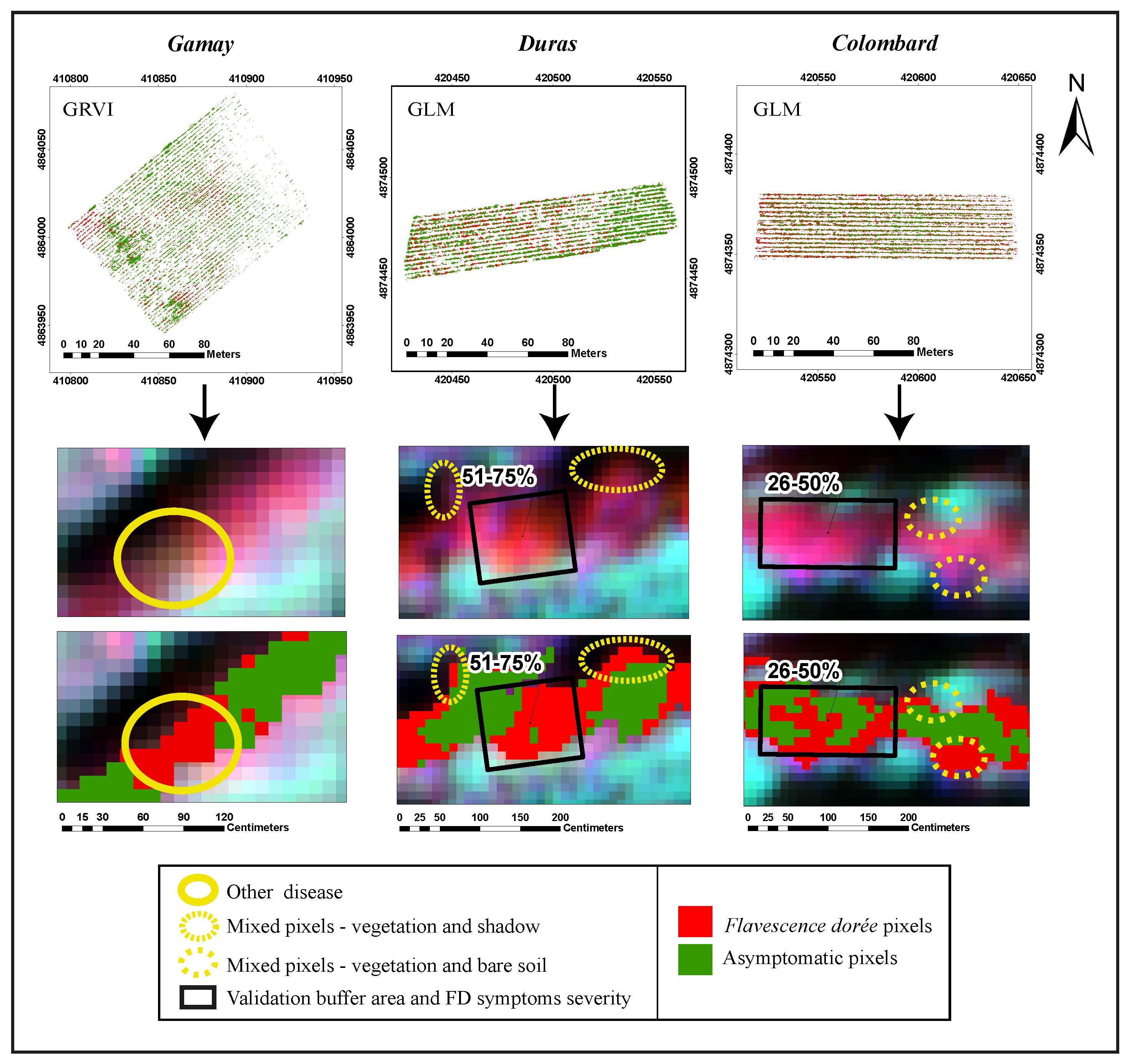
4.2. Application to Whole Vineyards and External Accuracy Assessment

Figure 6 presents for each vineyard (in column) a general overview of the classification result for all pixels labeled as ’grapevine vegetation’ (first row) and three subsets (second row) illustrating the main situations causing misclassification of true FD and AS pixels (second row). Even with the best classifiers, problems of true FD and AS pixel misclassifications remain as indicated by the FD_ds class difference between field and selected classifiers. The visual analysis of the FD maps realized with the best classifiers (selected from univariate or multivariate approaches) highlighted that main cause of misclassifications concern false FD pixels. Using higher spatial resolution (inferior to 8 cm) could improve the results when false FD pixels are confused with AS mixed pixels containing either grapevine vegetation and shadow.

When false FD pixels are confused with pixels presenting other similar colorations (either due stress or other diseases), adding one or several corresponding class(es) could be a way to improve the results. Additional field data, including observations for other diseases and stresses, are then clearly needed to verify if such classifiers could be useful to also discriminate FD from other diseases or nutritional disorders leading to similar leaves symptoms. It is only in this way that we can determine whether the use of UAV multispectral imagery is capable of specifically detecting the FD disease or whether its potential is limited to act as an alarm for anomalous coloring that would need to be checked in field to determine its origin.

4.3. Reproductibility of the Method

The method used to classify FD pixels was based on ROC curves. One of the main limitations of this method was the spatiotemporal consistency of the threshold. Values applied in here depended on the dataset and they are then probably specific to both year and vineyard. Such an approach means that a systematic calibration step is necessary, which limits the potentiality of this methodology. A calibration step is indeed not often possible in an operational context as data collection for this task is time- and labor-intensive. Complementary work (same cultivars and new cultivars in the same and another vine region) is necessary to really test the specificity of the thresholds to both year and vineyard.

5. Conclusions and Perspectives

Flavescence doree, with its rapid spread and the severe damage potential in major vine- and wine- producing European countries, is a major worldwide concern for grape producers. Finding a reliable operational method to identify FD-infected areas via remote sensing would improve the efficiency of removing infected plants and greatly limit the subsequent spread of the disease.

In this context, this study presents the potential of 20 variables (5 spectral bands, 11 vegetation indices and 4 biophysical parameters) computed from UAV multispectral imagery to remotely discriminate FD symptomatic from asymptomatic areas in four vineyards (red and white cultivars) in Southwest France. Receiver operator characteristic (ROC) analysis was used to determine the capacity of each variable to discriminate FD from AS pixels using both univariate and multivariate classification approaches. Contrasting results were obtained depending on red or white cultivars. On one hand, for the two white cultivars studied (Colombard and Cabernet Sauvignon), none of the variables tested (alone or combined into a GLM) provided satisfactory FD discrimination with a level of misclassification ranging between 10% and 20%. On the other hand, for the red cultivars (Gamay and Duras), two vegetation indices based on the green and red spectral bands—RGI and GRVI—and one biophysical parameter—Ant—linked to leaves anthocyanin concentration, showed a very high power of separability of FD and AS pixels. Level of misclassification was at worst 12%. Nevertheless, optimal thresholds vary for the two red cultivars studied in this work and this may limit the reproducibility of the proposed method. Whatever the cultivars (red or white), external accuracy assessment showed a systematic FD overestimation at parcel scale. Two main reasons were identified: FD pixels were confused either with pixels containing AS grapevine vegetation and shadow or pixels affected by other diseases presenting similar changes in leaf coloration.

Results are of great interest as no similar work on FD disease has yet been performed. However, in order to provide a reliable tool for FD management in the vine and wine production system, complementary investigation is needed to improve the robustness of the conclusions drawn here over the vineyards studied. This requires an increasing number of samples in future analyses, particularly for white cultivars for which the vineyards studied were little affected by the disease. For red cultivars, the very interesting results obtained also need to be confirmed with the same and other cultivars, over the same and different regions. Moreover, a challenge clearly remains to find a specific method to discriminate Flavescence doree from other vineyard diseases presenting similar changes in leaf coloration and this implies an exhaustive view of plot conditions. With these perspectives in mind, an intensive field campaign was completed in late summer 2016 over the Gaillac and the Minervois vineyard areas in Southwest France. Future work will mainly attempt to: (1) Confirm the high power of separability of FD and AS pixels obtained with the RGI and GRVI vegetation indices and the Ant biophysical parameter over other cultivars and another vine-growing region; (2) Test the specificity of the selected variables by adding a new class corresponding to grapevine trunk diseases; and (3) Use hyperspectral measurements carried out at the leaf scale in order to improve knowledge about the spectral response of symptomatic leaves (FD and grapevine trunk diseases), and to identify the most useful narrow bands for FD detection. Depending on these results, it might be possible to propose a specific spectral index based on actual UAV spectral bands, or to suggest specifications in terms of the number and width of bands to adapt existing sensors, or build future sensors for enhanced FD detection.

References

1. Chuche, J.; Thiéry, D. Biology and ecology of the Flavescence dorée vector Scaphoideus titanus: A review. Agron. Sustain. Dev. 2014, 34, 381. [Google Scholar] [CrossRef]
2. Schvester, D.; Carle, P.; Moutous, G. Sur la transmission de la Flavescence dorée des vignes par une cicadelle. Comptes Rendus des Séances de l’Académie d’Agriculture de France 1961, 47, 1021–1024. [Google Scholar]
3. Mori, N.; Bressan, A.; Martin, M.; Guadagnini, M.; Girolami, V.; Bertaccini, A. Experimental transmission by Scaphoideus titanus Ball of two Flavescence doree—Type phytoplasmas. VITIS J. Grapevine Res. 2002, 41, 99. [Google Scholar]
4. Bonfils, J.; Schvester, D. The leafhoppers (Homoptera: Auchenorrhyncha) and their relationship with vineyards in south-western France. Ann. Epiphyt. 1960, 11, 325–336. [Google Scholar]
5. Caudwell, A. Identification D’une Nouvelle Maladie à Virus de la Vigne, “la Flavescence dorée”, étude des Phénomènes de Localisation des Symptômes et de Rétablissement. Ph.D. Thesis, Institut National de la Recherche Agronomique, Paris, France, 1964. [Google Scholar]
6. Pavan, F.; Mori, N.; Bigot, G.; Zandigiacomo, P. Border effect in spatial distribution of Flavescence dorée affected grapevines and outside source of Scaphoideus titanus vectors. Bull. Insectol. 2012, 65, 281–290. [Google Scholar]
7. Jaunisses à phytoplasmes de la vigne. 2006. Available online: http://www.vignevin.com/fileadmin/users/ifv/publications/A_telecharger/JaunissesPhytoplasmesVigne.pdf (accessed on 30 December 2016).
8. GDON. Guide flavescence—Aide au diagnostic de la Flavescence dorée GDON du sauternais et des Graves; Technical Report; GDON du Sauternais et des Graves: Bordeaux, France, 2014. [Google Scholar]
9. Kazmi, S.J.H.; Usery, E.L. Application of remote sensing and GIS for the monitoring of diseases: A unique research agenda for geographers. Remote Sens. Rev. 2001, 20, 45–70. [Google Scholar] [CrossRef]
10. Franke, J.; Menz, G. Multi-temporal wheat disease detection by multi-spectral remote sensing. Precis. Agric. 2007, 8, 161–172. [Google Scholar] [CrossRef]
11. Sankaran, S.; Mishra, A.; Ehsani, R.; Davis, C. A review of advanced techniques for detecting plant diseases. Comput. Electron. Agric. 2010, 72, 1–13. [Google Scholar] [CrossRef]
12. Gennaro, S.F.D.; Battiston, E.; Marco, S.D.; Facini, O.; Matese, A.; Nocentini, M.; Palliotti, A.; Mugnai, L. Unmanned Aerial Vehicle (UAV)-based remote sensing to monitor grapevine leaf stripe disease within a vineyard affected by esca complex. Phytopathol. Mediterr. 2016, 55, 262–275. [Google Scholar]
13. Carter, G.A.; Knapp, A.K. Leaf optical properties in higher plants: Linking spectral characteristics to stress and chlorophyll concentration. Am. J. Bot. 2001, 88, 677–684. [Google Scholar] [CrossRef] [PubMed]
14. Naidu, R.A.; Perry, E.M.; Pierce, F.J.; Mekuria, T. The potential of spectral reflectance technique for the detection of Grapevine leafroll-associated virus-3 in two red-berried wine grape cultivars. Comput. Electron. Agric. 2009, 66, 38–45. [Google Scholar] [CrossRef]
15. Mahlein, A.K.; Oerke, E.C.; Steiner, U.; Dehne, H.W. Recent advances in sensing plant diseases for precision crop protection. Eur. J. Plant. Pathol. 2012, 133, 197–209. [Google Scholar] [CrossRef]
16. Yang, C.M.; Cheng, C.H.; Chen, R.K. Changes in spectral characteristics of rice canopy infested with brown planthopper and leaffolder. Crop Sci. 2007, 47, 329–335. [Google Scholar] [CrossRef]
17. Johnson, L.F.; Roczen, D.; Youkhana, S. Vineyard canopy density mapping with IKONOS satellite imagery. In Proceedings of the Third International Conference on Geospatial Information in Agriculture and Forestry, Denver, CO, USA, 5–7 November 2001. [Google Scholar]
18. Mirik, M.; Jones, D.; Price, J.A. Satellite Remote sensing of wheat infected by wheat streak mosaic virus. Plant Dis. 2011, 95, 4–12. [Google Scholar] [CrossRef]
19. Huang, W.; Lamb, D.W.; Niu, Z.; Zhang, Y.; Liu, L.; Wang, J. Identification of yellow rust in wheat using in-situ spectral reflectance measurements and airborne hyperspectral imaging. Precis. Agric. 2007, 8, 187–197. [Google Scholar] [CrossRef]
20. Reynolds, G.J.; Windels, C.E.; MacRae, I.V.; Laguette, S. Remote sensing for assessing Rhizoctonia crown and root rot severity in sugar beet. Plant Dis. 2012, 96, 497–505. [Google Scholar] [CrossRef]
21. Stilwell, A.R.; Hein, G.L.; Zygielbaum, A.I.; Rundquist, D.C. Proximal sensing to detect symptoms associated with wheat curl mite-vectored viruses. Int. J. Remote Sens. 2013, 34, 4951–4966. [Google Scholar] [CrossRef]
22. Zhang, M.; Qin, Z.; Liu, X.; Ustin, S.L. Detection of stress in tomatoes induced by late blight disease in California, USA, using hyperspectral remote sensing. Int. J. Appl. Earth Obs. Geoinf. 2003, 4, 295–310. [Google Scholar] [CrossRef]
23. MacDonald, S.L.; Staid, M.; Staid, M.; Cooper, M.L. Remote hyperspectral imaging of grapevine leafroll-associated virus 3 in cabernet sauvignon vineyards. Comput. Electron. Agric. 2016, 130, 109–117. [Google Scholar] [CrossRef]
24. Mazzetto, F.; Calcante, A.; Mena, A.; Vercesi, A. Integration of optical and analogue sensors for monitoring canopy health and vigour in precision viticulture. Precis. Agric. 2010, 11, 636–649. [Google Scholar] [CrossRef]
25. Colomina, I.; Molina, P. Unmanned aerial systems for photogrammetry and remote sensing: A review. ISPRS J. Photogramm. Remote Sens. 2014, 92, 79–97. [Google Scholar] [CrossRef]
26. Matese, A.; Toscano, P.; Di Gennaro, S.F.; Genesio, L.; Vaccari, F.P.; Primicerio, J.; Belli, C.; Zaldei, A.; Bianconi, R.; Gioli, B. Intercomparison of UAV, aircraft and satellite remote sensing platforms for precision viticulture. Remote Sens. 2015, 7, 2971–2990. [Google Scholar] [CrossRef]
27. Bock, C.H.; Nutter, F.W., Jr. Detection and measurement of plant disease symptoms using visible-wavelength photography and image analysis. CAB Rev. 2011, 6, 1–15. [Google Scholar] [CrossRef]
28. Steele, M.R.; Gitelson, A.A.; Rundquist, D.C.; Merzlyak, M.N. Nondestructive estimation of anthocyanin content in grapevine leaves. Am. J. Enol. Viticult. 2009, 60, 87–92. [Google Scholar]
29. Steele, M.R.; Gitelson, A.A.; Rundquist, D.C. A comparison of two techniques for nondestructive measurement of chlorophyll content in grapevine leaves. Agron. J. 2008, 100, 779–782. [Google Scholar] [CrossRef]
30. Blondlot, A.; Gate, P.; Poilvé, H. Providing operational nitrogen recommendations to farmers using satellite imagery. In Proceedings of the 5th European Conference on Precision Agriculture, Uppsala, Sweden, 9–12 June 2005; pp. 345–352. [Google Scholar]
31. Lacaze, R.; Baret, F.; Camacho, F.; d’Andrimont, R.; Freitas, S.C.; Pacholczyk, P.; Poilvé, H.; Smets, B.; Tansey, K.; Wagner, W. Geoland2—Towards an operational GMES land monitoring core service: The biogeophysical parameter core mapping service. In Proceedings of the 34th International Symposium on Remote Sensing of Environment, Sydney, Australia, 10–14 April 2011. [Google Scholar]
32. Chen, F.; Weber, K.T.; Anderson, J.; Gokhale, B. Comparison of MODIS fPAR products with Landsat-5 TM-derived fPAR over semiarid rangelands of Idaho. GISci. Remote Sens. 2010, 47, 360–378. [Google Scholar] [CrossRef]
33. Meroni, M.; Rembold, F.; Verstraete, M.M.; Gommes, R.; Schucknecht, A.; Beye, G. Investigating the relationship between the inter-annual variability of satellite-derived vegetation phenology and a proxy of biomass production in the Sahel. Remote Sens. 2014, 6, 5868–5884. [Google Scholar] [CrossRef]
34. Roumiguié, A.; Jacquin, A.; Sigel, G.; Poilvé, H.; Hagolle, O.; Daydé, J. Validation of a forage production index (FPI) derived from MODIS fCover time-series using high-resolution satellite imagery: Methodology, results and opportunities. Remote Sens. 2015, 7, 11525–11550. [Google Scholar] [CrossRef]
35. Poilvé, H. geoland2 BioPar Methods Compendium MERIS FR Biophysical Products; Technical Report BP-RP-BP038; VITO: Toulouse, France, 2010. [Google Scholar]
36. Jacquemoud, S.; Verhoef, W.; Baret, F.; Bacour, C.; Zarco-Tejada, P.J.; Asner, G.P.; François, C.; Ustin, S.L. PROSPECT+ SAIL models: A review of use for vegetation characterization. Remote Sens. Environ. 2009, 113, S56–S66. [Google Scholar] [CrossRef]
37. Jacquemoud, S.; Baret, F. PROSPECT: A model of leaf optical properties spectra. Remote Sens. Environ. 1990, 34, 75–91. [Google Scholar] [CrossRef]
38. Féret, J.B.; François, C.; Asner, G.P.; Gitelson, A.A.; Martin, R.E.; Bidel, L.P.; Ustin, S.L.; le Maire, G.; Jacquemoud, S. PROSPECT-4 and 5: Advances in the leaf optical properties model separating photosynthetic pigments. Remote Sens. Environ. 2008, 112, 3030–3043. [Google Scholar] [CrossRef]
39. Féret, J.B.; Noble, S.; Gitelson, A.; Jacquemoud, S. PROSPECT-Dynamic: Modeling leaf optical properties through a complete lifecycle. Remote Sens. Environ. 2017, 193, 204–215. [Google Scholar] [CrossRef]
40. Verhoef, W. Light scattering by leaf layers with application to canopy reflectance modeling: The SAIL model. Remote Sens. Environ. 1984, 16, 125–141. [Google Scholar] [CrossRef]
41. Rouse, J., Jr.; Haas, R.H.; Schell, J.A.; Deering, D.W. Monitoring vegetation systems in the Great Plains with ERTS. In Proceedings of the NASA Goddard Space Flight Center 3d ERTS-1 Symposium, Washington, DC, USA, 10–14 December 1973. [Google Scholar]
42. Gitelson, A.A.; Merzlyak, M.N.; Chivkunova, O.B. Optical properties and nondestructive estimation of anthocyanin content in plant leaves. Photochem. Photobiol. 2001, 74, 38–45. [Google Scholar] [CrossRef]
43. Gitelson, A.A.; Keydan, G.P.; Merzlyak, M.N. Three-band model for noninvasive estimation of chlorophyll, carotenoids, and anthocyanin contents in higher plant leaves. Geophys. Res. Lett. 2006, 33, L11402. [Google Scholar] [CrossRef]
44. Gamon, J.A.; Surfus, J.S. Assessing leaf pigment content and activity with a reflectometer. New Phytol. 1999, 143, 105–117. [Google Scholar] [CrossRef]
45. Van den Berg, A.K.; Perkins, T.D. Nondestructive estimation of anthocyanin content in autumn sugar maple leaves. HortScience 2005, 40, 685–686. [Google Scholar]
46. Gitelson, A.A.; Kaufman, Y.J.; Stark, R.; Rundquist, D. Novel algorithms for remote estimation of vegetation fraction. Remote Sens. Environ. 2002, 80, 76–87. [Google Scholar] [CrossRef]
47. Motohka, T.; Nasahara, K.N.; Oguma, H.; Tsuchida, S. Applicability of green-red vegetation index for remote sensing of vegetation phenology. Remote Sens. 2010, 2, 2369–2387. [Google Scholar] [CrossRef]
48. Huete, A.R. A soil-adjusted vegetation index (SAVI). Remote Sens. Environ. 1988, 25, 295–309. [Google Scholar] [CrossRef]
49. Gitelson, A.A.; Kaufman, Y.J.; Merzlyak, M.N. Use of a green channel in remote sensing of global vegetation from EOS-MODIS. Remote Sens. Environ. 1996, 58, 289–298. [Google Scholar] [CrossRef]
50. Richardson, A.J.; Wiegand, C.L. Distinguishing vegetation from soil background information. Photogramm. Eng. Remote Sens. 1977, 43, 1541–1552. [Google Scholar]
51. Tucker, C.J. Red and photographic infrared linear combinations for monitoring vegetation. Remote Sens. Environ. 1979, 8, 127–150. [Google Scholar] [CrossRef]
52. Huang, C.; Davis, L.S.; Townshend, J.R.G. An assessment of support vector machines for land cover classification. Int. J. Remote Sens. 2002, 23, 725–749. [Google Scholar] [CrossRef]
53. Saatchi, S.; Buermann, W.; Ter Steege, H.; Mori, S.; Smith, T.B. Modeling distribution of Amazonian tree species and diversity using remote sensing measurements. Remote Sens. Environ. 2008, 112, 2000–2017. [Google Scholar] [CrossRef]
54. Akaike, H. A new look at the statistical model identification. IEEE Trans. Autom. Control 1974, 19, 716–723. [Google Scholar] [CrossRef]
55. Collett, D. Modelling Binary Data; Chapman and Hall: London, UK, 1991. [Google Scholar]
56. Blackburn, G.A.; Steele, C.M. Towards the remote sensing of matorral vegetation physiology: Relationships between spectral reflectance, pigment, and biophysical characteristics of semiarid bushland canopies. Remote Sens. Environ. 1999, 70, 278–292. [Google Scholar] [CrossRef]
Figure 1. Location of the two study sites selected in southwestern France (A,B). Each site contains two vineyards of white (white polygons) and red cultivars (red polygons).
Remotesensing 09 00308 g001
Figure 2. Disease severity categories used in the field to report the percentage of a given vine presenting the symptoms of the Flavescence dorée. Four ordinal categories were established to express the Flavescence dorée disease severity (FDds1, FDds2, FDds3, FDds4).
Remotesensing 09 00308 g002
Figure 3. UAV images in false colors of the four selected vineyards (Gamay, Duras, Sauvignon and Colombard) acquired in September 2015 and localization of all infected grapevine. The size of the pink circles, which correspond to the ground-truth, varies according to the disease severity. The two pictures under each UAV image give an overview of the vineyard and show an example of an infected grapevine (with 76% to 100% of the vine presenting Flavescence dorée (FD) symptoms).
Remotesensing 09 00308 g003
Figure 4. Methodological framework with the main steps of data acquisition, processing and analysis. SB: spectral bands.
Remotesensing 09 00308 g004
Figure 5. Boxplots and optimal thresholds for selected variables for each vineyard.
Remotesensing 09 00308 g005
Figure 6. General overview of the classification result for all pixels labeled as ’grapevine vegetation’ over Gamay, Duras and Colombard vineyards (first row). Three subsets (second row) illustrate the main situations (other disease and mixed pixels) causing misclassifications of true FD and AS pixels. GLM: generalized linear models.
Remotesensing 09 00308 g006