Article

Spectroscopic Estimation of Biomass in Canopy Components of Paddy Rice Using Dry Matter and Chlorophyll Indices

National Engineering and Technology Center for Information Agriculture (NETCIA), Jiangsu Key Laboratory for Information Agriculture, Jiangsu Collaborative Innovation Center for Modern Crop Production, Nanjing Agricultural University, One Weigang, Nanjing 210095, China
*
Authors to whom correspondence should be addressed.
Remote Sens. 2017, 9(4), 319; https://doi.org/10.3390/rs9040319
Submission received: 28 December 2016 / Revised: 15 March 2017 / Accepted: 27 March 2017 / Published: 28 March 2017
(This article belongs to the Special Issue Remote Sensing of Above Ground Biomass)

Abstract

:
Crop biomass is a critical variable for characterizing crop growth development, understanding dry matter partitioning, and predicting grain yield. Previous studies on the spectroscopic estimation of crop biomass focused on the use of various spectral indices based on chlorophyll absorption features and found that they often became saturated at high biomass levels. Given that crop biomass is commonly expressed as the dry weight of canopy components per unit ground area, it may be better estimated using the spectral indices that directly characterize dry matter absorption. This study aims to evaluate a group of four dry matter indices (DMIs) by comparison with a group of four chlorophyll indices (CIs) for estimating the biomass of individual components (e.g., leaves, stems) and their combinations with the field data collected from a two-year rice cultivation experiment. The Red-edge Chlorophyll Index (CIRed-edge) of the CI group exhibited the best relationship with leaf biomass (R2 = 0.82) for the whole growing season and with total biomass (R2 = 0.81), but only for the growth stages before heading. However, the Normalized Difference Index for Leaf Mass per Area (NDLMA) of the DMI group showed the best relationships with both stem biomass (R2 = 0.81) and total biomass (R2 = 0.81) for the whole season. This research demonstrated the suitability of dry matter indices and provided physical explanations for the superior performance of dry matter indices over chlorophyll indices for the estimation of whole-season total biomass.

Graphical Abstract

1. Introduction

Rice has a critical role in ensuring food security for the largest population in the world [1]. Timely monitoring of rice growth status is crucial for global food security and agricultural sustainability [2]. Specifically, biomass can be used as an indicator of grain yield, growth status, and gross primary production [3,4]. Furthermore, the information on rice biomass is desired for calculating critical nitrogen (N) concentrations and also the nitrogen nutrition index, which is an important variable for in-season nitrogen management [5]. The traditional approach for measuring rice biomass by manually collecting physical samples is time consuming, labor intensive, and prone to errors. As a non-destructive approach, remote sensing has been successfully used to estimate the biomass of rice and other crops since the late 1990s [6,7].
The majority of previous studies on the remote estimation of crop biomass are based on several methods, including spectral vegetation indices (VIs) [6,7,8,9], multivariate regression [9,10], integration of remotely sensed data and crop growth models [11,12,13] or radiation use efficiency models [14], fusion of optical and radar data [15], and three-dimensional analysis of point cloud data [16,17]. The data-model integration methods are built on the physiological process of crop growth and can be used for estimating crop biomass under various growth and climate conditions, but much effort is required for parameterizing crop models and determining the optimal data assimilating strategy [18]. Crop biomass can be estimated with active remotely sensed data acquired from radar or LiDAR (light detection and ranging) instruments, but those data sources are often expensive and need extensive experiences for data processing [19]. Among all those methods, the use of various spectral VIs has been the most common one due to the simplicity of calculation and the widespread accessibility of spectral data. In the past two decades, most of the VIs for crop biomass estimation are calculated from either multispectral data collected with handheld sensors (e.g., CropScan, GreenSeeker, and Crop Circle) and satellite imagery (e.g., Landsat, RapidEye, and WorldView-2) or hyperspectral data collected with field spectroradiometers (e.g., ASD FieldSpec and Ocean Optics SD2000). The commonly used spectral indices from these data include the Normalized Difference Vegetation Index, NDVI [20,21], the Green NDVI [22], the Modified Chlorophyll Absorption in Reflectance Index, MCARI [23], the Red-edge Chlorophyll Index, CIRed-edge [23], red and red-edge reflectance-based indices [24,25], and near-infrared based indices [26]. In particular, the VIs derived from hyperspectral data are often variable between studies as a result of optimization in the form of NDVI with two new wavelengths for a specific data set, such as (R708 − R565)/(R708 + R565) [9], (R1301 − R1706)/(R1301 + R1706) [27], and (R752 − R549)/(R752 + R549) [28]. Those studies paid considerable attention to various types of indices originally designed for the detection of chlorophyll content, which was based on the chlorophyll absorption features in the red region.
As the crop biomass expressed in most studies is the dry weight of crop components per unit ground area, the physical variable that should be detected directly is actually the dry matter content instead of the chlorophyll content. However, it is still a common practice to use various chlorophyll indices for estimating crop biomass [7,8,9,10,11,12,13,14,15,16]. The estimation with these indices was indirect and its performance relied on the relationship between the biomass and chlorophyll content or leaf area index of crops [29,30]. If one uses the appropriate dry matter indices, a direct estimation should become possible and the estimation of crop biomass may be improved. Although a large number of VIs have been reported for estimating foliar chlorophyll content [31,32], only a few narrow-band indices have been developed specifically for detecting dry matter content. They were assessed with experimental and simulated data and proved to work well across a wide range of species [33,34]. These dry matter indices use one or two bands in the shortwave infrared (SWIR) region to characterize the dry matter absorption centered at 1.7 μm [35], and do not use any band in the visible and red edge regions as the chlorophyll indices do. To date, few studies have explicitly evaluated their performance for the estimation of crop biomass and the comparison of them to the commonly used chlorophyll indices. It is unclear whether and in what condition dry matter indices are more appropriate than chlorophyll indices for estimating crop biomass.
In addition, the biomass to be estimated with VIs is often from all the aboveground components of crops, including leaves, stems, and panicles or fruits. The aboveground biomass was found to be nonlinearly related to the chlorophyll indices [9,22,26]. These nonlinear relationships could be due to the poor sensitivity of chlorophyll indices to the aboveground biomass at high biomass levels and could lead to large uncertainties in the biomass estimation. Because of the strong interest in the aboveground biomass, the common practice in the community is still to estimate the biomass of all individual components as a whole using various chlorophyll indices [30]. This problem may be alleviated by exploiting dry matter indices for the spectroscopic estimation and decomposing the aboveground biomass into individual components such as leaf biomass and stem biomass for the evaluation.
Given the smaller amount of mass per unit ground area in leaf biomass than in total biomass, the poor sensitivity of VIs to total biomass at high levels may be better understood by an additional examination of the leaf biomass. The recent research by Kross et al. [25] represented one of the few attempts of this kind and investigated this possibility in corn and soybean crops. Although a number of studies have focused on the estimation of total biomass specifically in rice [6,23,24,27,28], none of them have taken the investigation of individual components in total biomass into consideration. Therefore, particular attention should be paid to the difference in performance between the spectroscopic estimation of total biomass and those of biomass for individual components in rice. Moreover, those pertinent investigations included very few or even no data samples collected after the heading stage and were unable to cover the whole growing season of rice. Considering the high biomass at the post-heading stages of the season, it becomes important to determine whether the models for biomass estimations could be fitted across all critical stages or only for specific stages of the whole season.
The objectives of this study were to evaluate the performance of dry matter indices in comparison with chlorophyll indices for the estimation of leaf biomass, stem biomass, and total biomass in rice and to evaluate the feasibility of fitting a single index-based model across all growth stages of the growing season. Eight spectral indices selected from the literature for such a purpose were evaluated with a large number of samples collected from a two-year experiment for the whole growing season of rice.

2. Materials and Methods

2.1. Experimental Design

The experiment was designed for two consecutive years with the same treatments, involving different rice cultivars, planting densities, and nitrogen (N) rates. The crops were grown in 2014 and 2015 in the same fields at the experimental station of the National Engineering and Technology Center for Information Agriculture (NETCIA), Rugao, Jiangsu, China (120°19′E, 32°14′N). There were four N rate treatments (0, 100, 200, and 300 kg·N·ha−1) with the density of 0.30 m × 0.15 m for the minimum and maximum rates and two densities (0.30 m × 0.15 m and 0.50 m × 0.15 m) for the intermediate rates. The N fertilizers were applied in the form of urea: 40% as basal fertilizer before transplanting, 10% at the tillering stage, 30% at the jointing stage, and 20% at the booting stage. The two rice cultivars involved were Y liangyou 1 (Indica rice, V1) and Wuyunjing 24 (Japonica rice, V2). Each plot was 5 m × 6 m in size. A total of 36 plots (12 cultivation conditions with three replications) were grown for the whole study in each year.

2.2. Spectral Measurements

Spectral reflectance was measured with an ASD FieldSpec Pro spectrometer (Analytical Spectral Devices, Boulder, CO, USA) with a 25° field of view at a height of 1.0 m above the rice canopy. The spectral range was 350–2500 nm, with a 1.4 nm sampling interval between 350 and 1050 nm and a 2 nm sampling interval between 1000 and 2500 nm. Spectral measurements were taken from 11:00 a.m. to 1:00 p.m. local time. There were three observation points fixed in each plot and each point was measured five times with the ASD spectrometer. The mean of those measurements was calculated to represent the reflectance spectrum of each plot. Calibration measurements were done with a white reference panel every ten minutes. A summary of the sampling dates is listed in Table 1.

2.3. Biomass Measurements

The samples of all canopy components at each growth stage were collected within one day of the spectral measurements. For each plot, three hills of plants at the center of the spectral sampling area were cut at the ground surface. All green leaves and panicles when present were separated from the stems. All components were oven-dried at 105 °C for 30 min and then at 80 °C for about 24 h until a constant weight was obtained. A total of 359 leaf samples, 359 stem samples, and 96 panicle samples were collected in the two years at the growth stages of early tillering, late tillering, jointing, early booting, late booting, heading, early filling, and late filling (Table 2).

2.4. Calculation of Spectral Indices and Estimation of Biomass

Two groups of vegetation indices (VIs) (Table 3) were calculated with the spectral data. One was the group of chlorophyll indices (CIs), including the Red-edge Chlorophyll Index, CIred edge [36], the ratio of Transformed Chlorophyll Absorption in Reflectance Index to Optimized Soil-Adjusted Vegetation Index, TCARI/OSAVI [37], the Normalized Difference Vegetation Index, NDVI [38], and the Enhanced Vegetation Index, EVI [39]. They were selected to represent the red-edge based indices, soil-resistant indices, and the two most commonly used vegetation indices. The other was the group of dry matter indices (DMIs), including the Normalized Difference index for the Leaf Mass per Area, NDLMA [33], the Normalized Dry Matter Index, NDMI [34], the Normalized Difference Lignin Index, NDLI [40], and the Normalized Difference Index for leaf canopy biomass, NDBleaf [41]. The DMIs represented all significant developments in dry matter estimation reported in the literature and were less commonly used in the community due to the use of SWIR bands. To keep the balance between the two groups, this study retained only those four chlorophyll indices although more were available in the literature. The selection of four indices for each group ensured that reasonable representations and adequate attention was paid to their specific relationships with the biomass for the individual and multiple components.
The data collected from the two-year experiment were pooled to examine the relationships between the eight vegetation indices and the biomass of different components or component combinations. Linear and nonlinear (exponential) models were developed to fit those relationships. The predictive capability of those models were assessed by the Root Mean Square Error (RMSE) using a k-fold (k = 10) cross-validation procedure.

3. Results

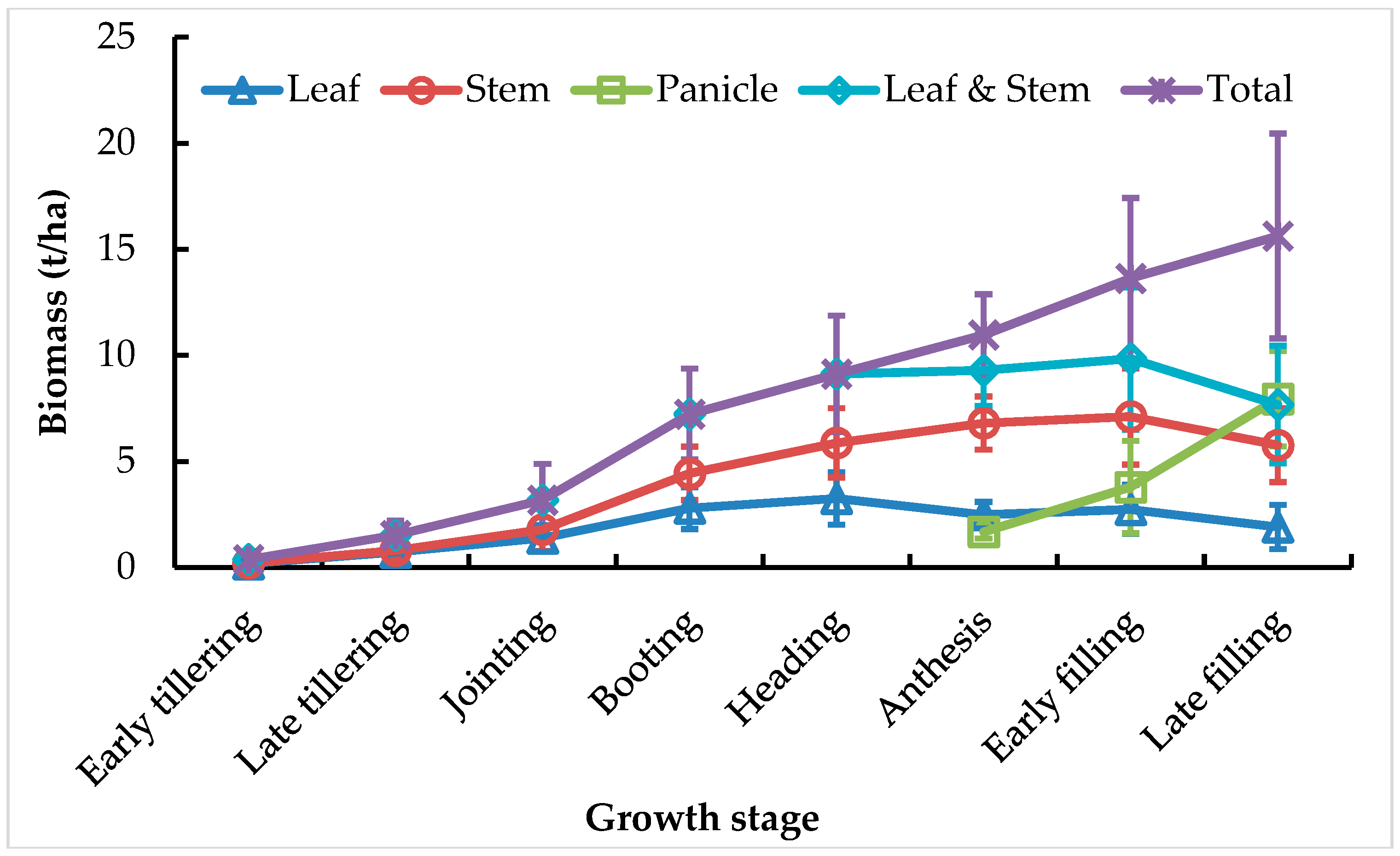
3.1. Variation in Biomass of Individual and Multiple Components over the Growing Season

The temporal patterns of biomass measurements across the stages are displayed in Figure 1. The leaf biomass increased gradually from the early tillering stage to the late booting stage and decreased to the minimum at the late filling stage. The stem biomass kept increasing until the early filling stage and also decreased at the late filling stage. The difference between mean leaf biomass and mean stem biomass was greater for the post-heading (heading included) stages than that for the pre-heading (heading excluded) stages. Panicle biomass increased from the heading stage to the late filling stage and exceeded stem biomass at the late filling stage. The biomass of leaves and stems increased rapidly from the early tillering stage to the heading stage and remained almost stable until the decrease from the early filling stage to the late filling stage. The total biomass increased with the growth stage for the whole season.

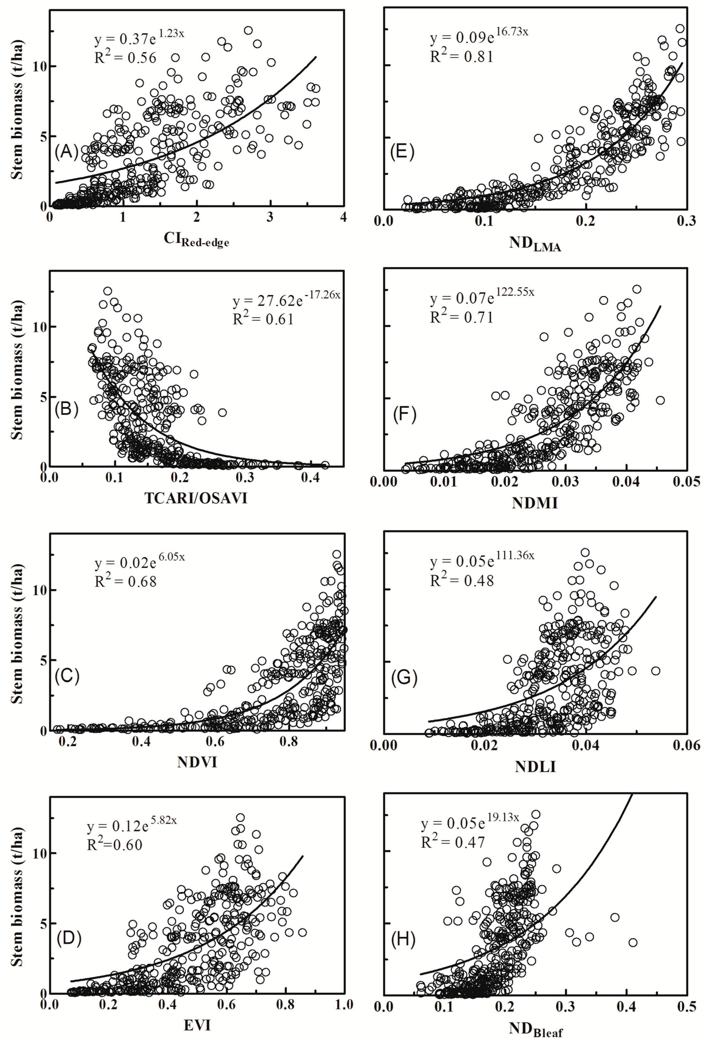
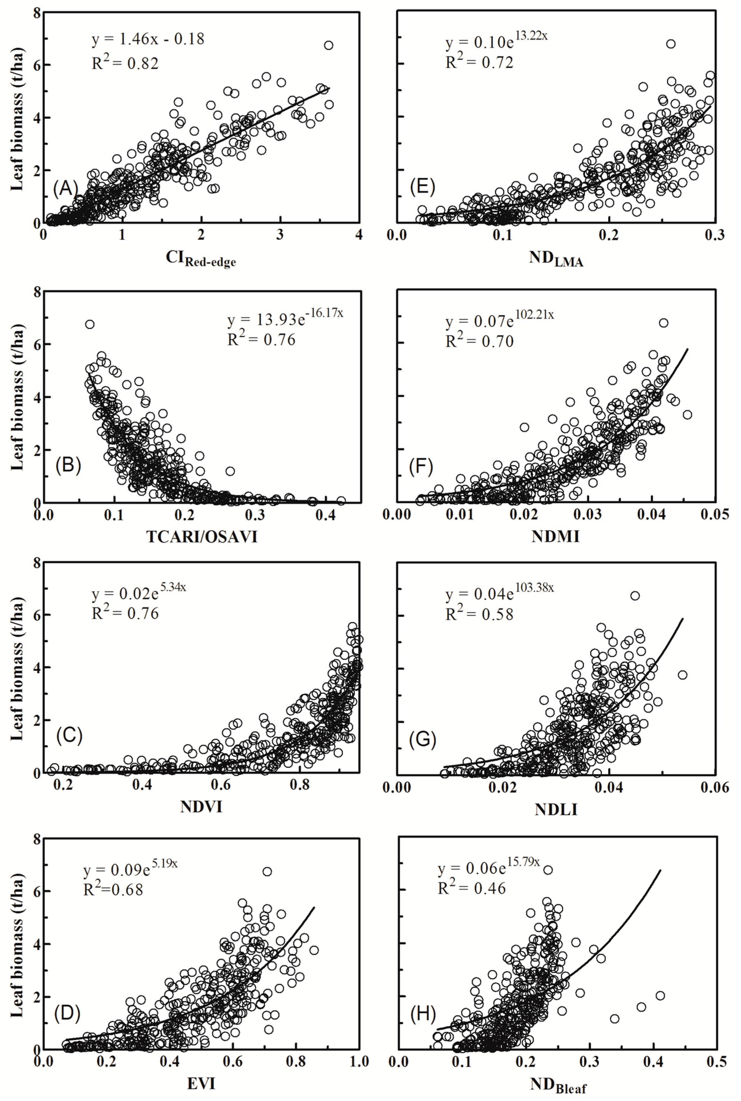
3.2. Relationships between Vegetation Indices and Biomass of Individual Components

The best-fit functions for the relationships between the vegetation indices and leaf biomass were mostly nonlinear with R2 values ranging from 0.68 to 0.82 for chlorophyll indices and from 0.46 to 0.72 for dry matter indices. Only the CIred edge from the CI group exhibited linear relationships with the leaf biomass (Figure 2A), even with the best goodness of fit of all indices examined. The TCARI/OSAVI and the NDVI exhibited a strong relationship with the leaf biomass but the sensitivity decreased considerably when the leaf biomass exceeded 1 t/ha (Figure 2B,C). The relationships of the leaf biomass with EVI (Figure 2D) and all indices from the DMI group showed similar asymptotic patterns, but with various degrees of the scattering of data points from the nonlinear fits. Within the DMI group, the NDLMA and the NDMI showed better fits with leaf biomass than the NDLI and the NDBleaf (Figure 2E–H).
Unlike leaf biomass, stem biomass was nonlinearly related to all of the eight spectral indices. The relationships of the stem biomass with CIRed-edge showed an even higher scattering of data points than those with the NDVI and the EVI (Figure 3A–D). The sensitivity of NDVI to the stem biomass became poor when the stem biomass exceeded 2.5 t/ha. The NDLMA from the DMI group showed the strongest relationship (R2 = 0.81, p < 0.001) with stem biomass than any other index evaluated (Figure 3E–H). This indicates that the best chlorophyll index examined is more suitable than the best dry matter index for the estimation of leaf biomass, but not for the estimation of stem biomass. In contrast to the leaf biomass and stem biomass, the panicle biomass was not significantly related to any of the spectral indices (data not shown).

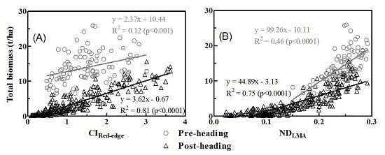
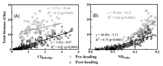
3.3. Relationships between Vegetation Indices and Biomass of Multiple Components

The relationships of the spectral indices with the biomass of the leaf and stem components showed similar patterns to those with the leaf biomass (Table 4), exhibiting linear best-fits for the CIRed-edge and nonlinear best-fits for other indices. The goodness of fits decreased after the addition of the stem biomass for all chlorophyll indices, particularly for the CIRed-edge. In contrast, the goodness of fit for three of the four DMIs increased with the R2 for the NDLMA being the greatest (0.72 to 0.79).
With regards to the total biomass of the aboveground components, all the best-fit functions were nonlinear and the best fit of all was with the NDLMA (R2 = 0.81) (Table 4). This suggests that the best dry matter index examined is a better indicator of the biomass across the whole season than the best chlorophyll index for multiple components. Closer examinations of the nonlinear relationships showed that the nonlinearity for the NDLMA across the whole season encompassed two linear fits divided by the growth stage, with one for pre-heading and the other for the post-heading stages. From the transition of the pre-heading phase to the post-heading phase, the change in total biomass appeared faster with the NDLMA (pre-heading: slope = 44.89; post-heading: slope = 99.26) but became slower with the CIRed-edge (pre-heading: slope = 3.62; post-heading: slope = 2.37) as measured by the slopes of the regression lines (Figure 4). The CIRed-edge exhibited the highest correlation (R2 = 0.81) of all indices with the total biomass for the stages before heading (Figure 4A), followed by the NDLMA (R2 = 0.75). For the stages after heading, the NDLMA exhibited the highest correlation (R2 = 0.46) (Figure 4B), which was substantially greater than the correlations with any other chlorophyll index (R2 ranging from 0.06 to 0.19).

3.4. Model Validation

For the estimation of leaf biomass with the best-fit models as shown in Figure 2, the CIRed-edge exhibited the lowest RMSE (RMSE = 0.56 t/ha) which was lower than those obtained with the NDLMA (RMSE = 0.75 t/ha) and other indices. For the estimation of stem biomass, the lowest RMSE was produced by the NDLMA among all indices (Table 5). The NDLMA also exhibited the lowest RMSE values for the estimation of the leaf and stem biomass (RMSE = 1.99 t/ha) and of the total biomass across all growth stages (RMSE = 3.07 t/ha). In the CI group, the CIRed-edge performed best with an RMSE of 2.42 t/h for the estimation of the leaf and stem biomass but produced the highest RMSE (8.29 t/ha) for the total biomass. While calibrating linear models by two groups of growth stages, the NDLMA still produced the most accurate estimation of the total biomass for the post-heading group(RMSE = 3.19 t/ha) and the second most accurate estimation for the pre-heading group (RMSE = 1.75 t/ha), which was close to the most accurate estimation with the CIRed-edge (RMSE = 1.51 t/ha).

4. Discussion

4.1. Why Did Dry Matter Indices Work Better Than Chlorophyll Indices?

As the chlorophyll in green leaves is a major absorber of solar radiation within crop canopies, chlorophyll indices are widely used for estimating crop growth parameters such as leaf area index [20] and leaf nitrogen content [9,42] based on their correlations with the leaf chlorophyll content. The CIRed-edge is one such index and relies primarily on the sensitivity of red edge bands to chlorophyll absorption [36]. Our results demonstrated that the chlorophyll indices performed well in the estimation of leaf biomass but not better than the dry matter index NDLMA in the estimation of the total biomass, due to their difficulties in accounting for the variation in stem biomass.
Since the biomass in this study was the mass of dry matter per unit ground area, the relationships of crop biomass with chlorophyll indices were indirect but those with dry matter indices were direct. Although the CIRed-edge exhibited significant relationships with leaf biomass, the strength decreased when the stem biomass was included. The explicit examination of the relationships of stem biomass and total biomass with the CIRed-edge confirmed the breakdown of this indirect connection.
The stable performance of the NDLMA for estimating the biomass of individual and multiple organs in rice canopies suggested that the use of a sensitive dry matter index was a successful choice. On one hand, the NDLMA was originally designed by Féret et al. [33] as an indicator of leaf dry matter content and involved a combination of one NIR band (1320 nm) and one SWIR band (1722 nm). Swain et al. [43] also found that this SWIR band was sensitive to dry matter content as used in their index, NDMI. These dry matter indices expectedly performed better than the chlorophyll indices for the estimation of total biomass. A recent study by Jin et al. [18] showed the better performance of the NDMI for biomass estimation than a few chlorophyll indices, but did not consider the NDLMA. Gnyp et al. [27] determined (R1301 − R1706)/(R1301 + R1706), of which the two bands were approximately 20 nm offset from their counterparts in the NDLMA, as their best wavelength combination for the estimation of the total biomass in rice. An analysis of our data demonstrated that their index performed similarly (R2 = 0.81) as did the NDLMA, but exhibited a different model. Although Gnyp et al. [27] did not explicitly link the optimized index to dry matter detection, the successful performance of this index reinforced the suitability of dry matter indices for biomass estimation.
On the other hand, it is common practice to use a spectral index with higher sensitivity to a constituent for detecting low concentrations, but with lower sensitivity to this constituent for detecting high concentrations, as a strategy to avoid optical saturation [36,44]. From the pre-heading phase to the post-heading phase, the total biomass increased to a much higher level (more than doubled) but the CIRed-edge failed to respond to this physiological process (Figure 4A). Compared to the red edge band (700 nm) in the CIRed-edge and the TCARI/OSAVI, the SWIR band (1722 nm) used in the NDLMA and the NDMI exhibited higher reflectance and could be more efficient for detecting dry matter signals from stems that are located deeper in the canopy than the leaves at the top. Although stems could barely be visible from the top of the canopy, dry matter signals could come from the multiple scattering of photons between leaves and stems.

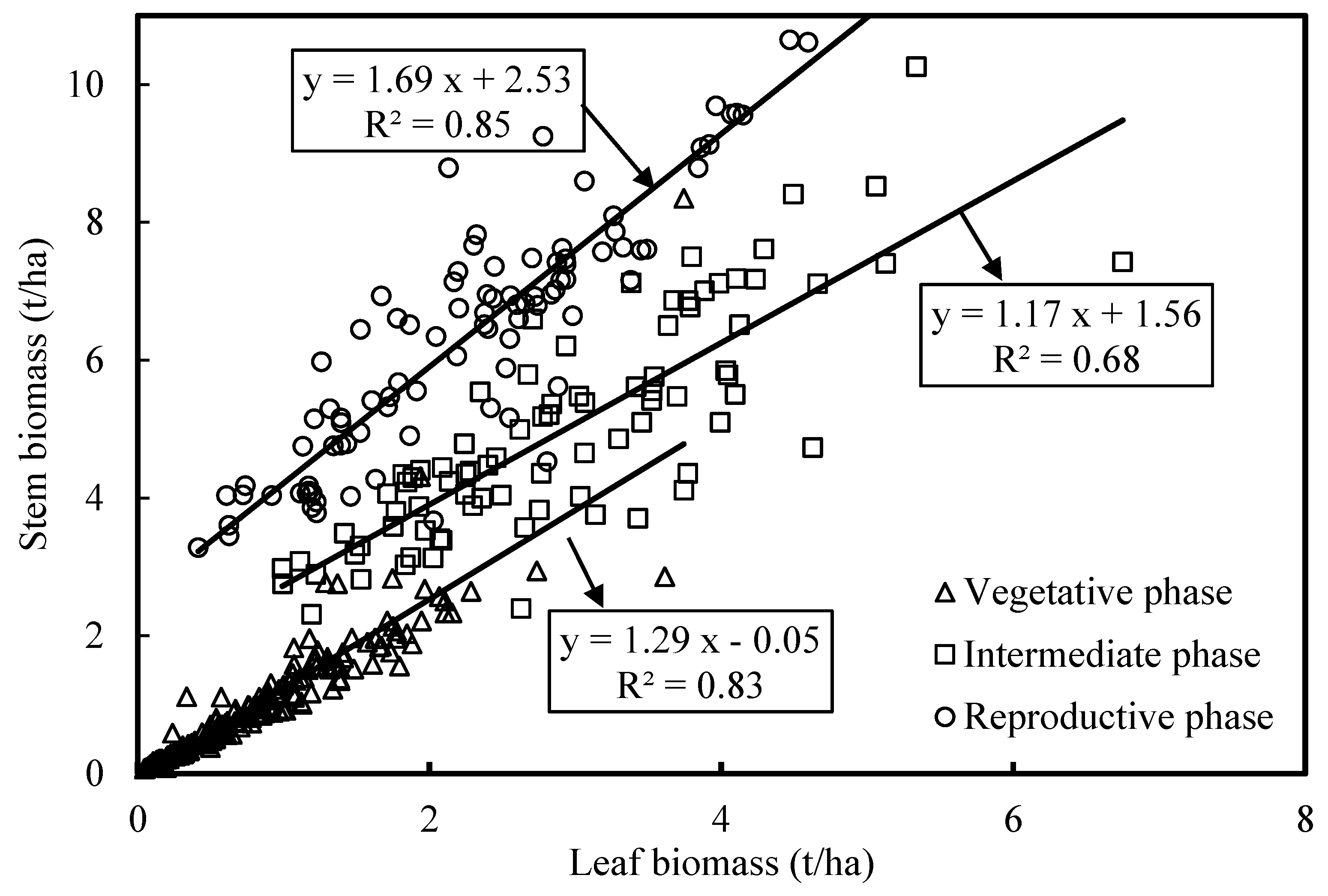
4.2. Partitioning of Aboveground Biomass between Canopy Components

The total biomass of the aboveground components of the canopy is a critical parameter for quantifying nitrogen deficiencies and the harvest index in crops [45,46,47]. Starting from the booting stage, rice plants transitioned to the reproductive growth phase, which is dominated by grain development with the translocation of dry matter from leaves and stems to panicles. Stem biomass contributed the most to the total biomass for all stages except at the start and the end of the growing season.
To this end, most studies for precision agriculture purposes focus on the remote estimation of total biomass but the estimation of individual components comprising the total biomass is poorly understood. To the best of our knowledge, this study provided the first attempt for the remote estimation for individual components towards a better understanding of the remote estimation of the total biomass. The relationships between the leaf biomass and vegetation indices could be explained by the absorption by dry matter in the leaves or by chlorophyll which is closely related to the leaf biomass of green crops. However, the relationships between stem biomass and vegetation indices could probably be explained by dry matter absorption and the allometric relationships between stem biomass and leaf biomass, given the low exposure of standing stems to the sensor. This leaf vs. stem biomass relationship was strong for the rice plants, but varied with the growth stage (Figure 5).
Our analysis indicated the leaf vs. stem relationships existed separately for at least three periods (i.e., vegetative, intermediate, and reproductive stages) comprising the whole season, with more significant differences in the offset than in the slope between these linear models. The partitioning of aboveground biomass among the leaf, stem, and panicle components of rice is dependent on the growth stage [48], therefore it was unrealistic to apply a single relationship for the whole growing season. This stage-specific relationship could probably explain the worse performance of the CIRed-edge in the estimation of stem biomass than that of leaf biomass. While a single linear function could explain the relationship between the leaf biomass and the CIRed-edge across all stages, even a nonlinear function could not well explain the relationship between the CIRed-edge and stem biomass (Figure 3A). As the NDLMA was used to directly detect the dry matter signals from all aboveground components of the rice plants, the partitioning pattern of dry matter among canopy components did not significantly affect the performance of the NDLMA in the estimation of stem biomass and total biomass. The non-significant relationship between panicle biomass and spectral indices suggested the limited contribution of the rice panicles to canopy spectral reflectance. Since the panicles were located on the upper layer of the crops, it was difficult for them to trap photons and therefore be detected by the sensor from above the canopy.

4.3. Potential for Satellite Observations

Most previous studies on the estimation of crop biomass used vegetation indices constructed with spectral bands in the visible and NIR regions, due to the limitation of the wavelength configuration of satellite instruments [25,28]. With the red edge indices derived from RapidEye image data, Kross et al. [25] also found linear fitting for the leaf biomass and nonlinear fitting for the total biomass in soybean and corn crops. Their finding from satellite observations was consistent with our results regarding the CIRed-edge derived from ground-based canopy reflectance spectra.
Our results suggested that the red edge indices were better suited for the estimation of leaf biomass than regular NDVI-like indices (without red edge bands) because of the high sensitivity of red edge indices to leaf biomass across all growth stages. For satellite mapping of crop leaf biomass, the red edge indices can be computed from multispectral images acquired from the instruments such as WorldView-2 [28], RapidEye [25], Sentinel-2 [49], and the Medium Resolution Imaging Spectrometer, MERIS [50]. These satellite-based red edge indices also have the potential for accurate estimation of total biomass for pre-heading stages. If the satellite mapping of the total biomass for the whole rice season is required, the bands for the NDLMA are preferred in order to avoid unsatisfactory estimates for the post-heading stages. Once the upcoming hyperspectral satellite missions such as the Environmental Mapping and Analysis Program, EnMap [51] and the Hyperspectral Infrared Imager, HyspIRI [52] are launched into orbit, the NDLMA and other optimal dry matter indices will be available for monitoring the aboveground biomass of rice and even other crops for the whole growing season.

5. Conclusions

This study reports on an investigation of the relationships between vegetation indices and the biomass of individual components and component combinations in rice canopies. Eight indices commonly used for the estimation of chlorophyll and dry matter contents were evaluated with field data collected from a two-year experiment. The CIRed-edge of the chlorophyll index group exhibited the best relationship (linear) of all with the leaf biomass for the whole rice season, and with total biomass, but only for the growth stages before heading due to the poor sensitivity to the large amount of total biomass after heading. The NDLMA of the dry matter index group showed the best relationships (nonlinear) with both stem biomass and total biomass for the whole season. Therefore, the use of canopy sensors that record NDVI or red-edge index data will either be limited to the monitoring of leaf biomass for the whole season or to that of total biomass for the stages before heading. The findings may serve as a guide to choose sensors with appropriate spectral coverages for monitoring the leaf biomass and total biomass for the growing season of rice.
With the detailed analysis of biomass estimation by the components in rice, this research provided physical explanations for the superior performance of the dry matter indices over the chlorophyll indices for the estimation of whole-season total biomass. The dry matter indices, particularly the NDLMA, can serve as useful spectral indicators of biomass for understanding the dry matter or carbon partitioning among aboveground components and the formation of grain yield of rice and other crops. They have great potential for the mapping of crop aboveground biomass for the whole growing season when spectroscopic data from upcoming hyperspectral satellite missions become available.

Acknowledgments

This research was funded by the National Key R&D Program (2016YFD0300601), the Fundamental Research Funds for the Central Universities (KYRC201401), the National Natural Science Foundation of China (31470084), Jiangsu Distinguished Professor Program, Special Program for Agriculture Science and Technology from Ministry of Agriculture in China (201303109), and the Academic Program Development of Jiangsu Higher Education Institutions (PAPD). Field assistance from graduate students Xiang Zhou and Xinqiang Deng is appreciated.

Author Contributions

T.C., X.Y., Y.T., W.C., and Y.Z. conceived and designed the experiments; D.L., K.Z., and H.Z. performed the experiments; T.C., R.S., and D.L. analyzed the data; D.L. provided analysis tools, T.C., R.S., and K.Z. wrote the paper.

Conflicts of Interest

The authors declare no conflict of interest.

References

  1. Cantrell, R.P.; Reeves, T.G. The cereal of the world’s poor takes center stage. Science 2002, 296, 53–53. [Google Scholar] [CrossRef] [PubMed]
  2. Zhao, G.; Miao, Y.; Wang, H.; Su, M.; Fan, M.; Zhang, F.; Jiang, R.; Zhang, Z.; Liu, C.; Liu, P. A preliminary precision rice management system for increasing both grain yield and nitrogen use efficiency. Field Crop. Res. 2013, 154, 23–30. [Google Scholar] [CrossRef]
  3. Harrell, D.; Tubana, B.; Walker, T.; Phillips, S. Estimating rice grain yield potential using normalized difference vegetation index. Agron. J. 2011, 103, 1717–1723. [Google Scholar] [CrossRef]
  4. Peng, Y.; Gitelson, A.A. Application of chlorophyll-related vegetation indices for remote estimation of maize productivity. Agric. For. Meteorol. 2011, 151, 1267–1276. [Google Scholar] [CrossRef]
  5. Chen, P.; Haboudane, D.; Tremblay, N.; Wang, J.; Vigneault, P.; Li, B. New spectral indicator assessing the efficiency of crop nitrogen treatment in corn and wheat. Remote Sens. Environ. 2010, 114, 1987–1997. [Google Scholar] [CrossRef]
  6. Thenkabail, P.S.; Smith, R.B.; De Pauw, E. Hyperspectral vegetation indices and their relationships with agricultural crop characteristics. Remote Sens. Environ. 2000, 71, 158–182. [Google Scholar] [CrossRef]
  7. Casanova, D.; Epema, G.F.; Goudriaan, J. Monitoring rice reflectance at field level for estimating biomass and lai. Field Crop Res. 1998, 55, 83–92. [Google Scholar] [CrossRef]
  8. Serrano, L.; Filella, I.; Penuelas, J. Remote sensing of biomass and yield of winter wheat under different nitrogen supplies. Crop Sci. 2000, 40, 723–731. [Google Scholar] [CrossRef]
  9. Hansen, P.M.; Schjoerring, J.K. Reflectance measurement of canopy biomass and nitrogen status in wheat crops using normalized difference vegetation indices and partial least squares regression. Remote Sens. Environ. 2003, 86, 542–553. [Google Scholar] [CrossRef]
  10. Fu, Y.Y.; Yang, G.J.; Wang, J.H.; Song, X.Y.; Feng, H.K. Winter wheat biomass estimation based on spectral indices, band depth analysis and partial least squares regression using hyperspectral measurements. Comput. Electron. Agric. 2014, 100, 51–59. [Google Scholar] [CrossRef]
  11. Dong, T.F.; Liu, J.G.; Qian, B.D.; Jing, Q.; Croft, H.; Chen, J.M.; Wang, J.F.; Huffman, T.; Shang, J.L.; Chen, P.F. Deriving maximum light use efficiency from crop growth model and satellite data to improve crop biomass estimation. IEEE J. Sel. Top. Appl. Earth Obs. Remote Sens. 2017, 10, 104–117. [Google Scholar] [CrossRef]
  12. He, B.B.; Li, X.; Quan, X.W.; Qiu, S. Estimating the aboveground dry biomass of grass by assimilation of retrieved lai into a crop growth model. IEEE J. Sel. Top. Appl. Earth Obs. Remote Sens. 2015, 8, 550–561. [Google Scholar] [CrossRef]
  13. Jego, G.; Pattey, E.; Liu, J.G. Using leaf area index, retrieved from optical imagery, in the stics crop model for predicting yield and biomass of field crops. Field Crop. Res. 2012, 131, 63–74. [Google Scholar] [CrossRef]
  14. Liu, J.G.; Pattey, E.; Miller, J.R.; McNairn, H.; Smith, A.; Hu, B.X. Estimating crop stresses, aboveground dry biomass and yield of corn using multi-temporal optical data combined with a radiation use efficiency model. Remote Sens. Environ. 2010, 114, 1167–1177. [Google Scholar] [CrossRef]
  15. Jin, X.L.; Yang, G.J.; Xu, X.G.; Yang, H.; Feng, H.K.; Li, Z.H.; Shen, J.X.; Zhao, C.J.; Lan, Y.B. Combined multi-temporal optical and radar parameters for estimating lai and biomass in winter wheat using HJ and RadarSAT-2 data. Remote Sens. 2015, 7, 13251–13272. [Google Scholar] [CrossRef]
  16. Bendig, J.; Bolten, A.; Bennertz, S.; Broscheit, J.; Eichfuss, S.; Bareth, G. Estimating biomass of barley using Crop Surface Models (CSMs) derived from UAV-based RGB imaging. Remote Sens. 2014, 6, 10395–10412. [Google Scholar] [CrossRef]
  17. Eitel, J.U.H.; Magney, T.S.; Vierling, L.A.; Brown, T.T.; Huggins, D.R. Lidar based biomass and crop nitrogen estimates for rapid, non-destructive assessment of wheat nitrogen status. Field Crop. Res. 2014, 159, 21–32. [Google Scholar] [CrossRef]
  18. Jin, X.; Kumar, L.; Li, Z.; Xu, X.; Yang, G.; Wang, J. Estimation of winter wheat biomass and yield by combining the AquaCrop model and field hyperspectral data. Remote Sens. 2016, 8, 972. [Google Scholar] [CrossRef]
  19. Wiseman, G.; McNairn, H.; Homayouni, S.; Shang, J.L. Radarsat-2 polarimetric SAR response to crop biomass for agricultural production monitoring. IEEE J. Sel. Top. Appl. Earth Obs. Remote Sens. 2014, 7, 4461–4471. [Google Scholar] [CrossRef]
  20. Li, F.; Etc, Y.M.; Li, F. Estimating winter wheat biomass and nitrogen status using an active crop sensor. Intell. Autom. Soft Comput. 2010, 16, 1221–1230. [Google Scholar]
  21. Wang, L.A.; Zhou, X.; Zhu, X.; Dong, Z.; Guo, W. Estimation of biomass in wheat using random forest regression algorithm and remote sensing data. Crop J. 2016, 4, 212–219. [Google Scholar] [CrossRef]
  22. Prabhakara, K.; Hively, W.D.; McCarty, G.W. Evaluating the relationship between biomass, percent groundcover and remote sensing indices across six winter cover crop fields in Maryland, United States. Int. J. Appl. Earth Obs. Geoinf. 2015, 39, 88–102. [Google Scholar] [CrossRef]
  23. Cao, Q.; Miao, Y.; Wang, H.; Huang, S.; Cheng, S.; Khosla, R.; Jiang, R. Non-destructive estimation of rice plant nitrogen status with crop circle multispectral active canopy sensor. Field Crop. Res. 2014, 154, 133–144. [Google Scholar] [CrossRef]
  24. Kanke, Y.; Tubaña, B.; Dalen, M.; Harrell, D. Evaluation of red and red-edge reflectance-based vegetation indices for rice biomass and grain yield prediction models in paddy fields. Precis. Agric. 2016, 17, 507–530. [Google Scholar] [CrossRef]
  25. Kross, A.; Mcnairn, H.; Lapen, D.; Sunohara, M.; Champagne, C. Assessment of rapideye vegetation indices for estimation of leaf area index and biomass in corn and soybean crops. Int. J. Appl. Earth Obs. Geoinf. 2015, 34, 235–248. [Google Scholar] [CrossRef]
  26. Gnyp, M.L.; Bareth, G.; Li, F.; Lenz-Wiedemann, V.I.S.; Koppe, W.; Miao, Y.; Hennig, S.D.; Jia, L.; Laudien, R.; Chen, X.; et al. Development and implementation of a multiscale biomass model using hyperspectral vegetation indices for winter wheat in the north China plain. Int. J. Appl. Earth Obs. Geoinf. 2014, 33, 232–242. [Google Scholar] [CrossRef]
  27. Gnyp, M.L.; Miao, Y.X.; Yuan, F.; Ustin, S.L.; Yu, K.; Yao, Y.K.; Huang, S.Y.; Bareth, G. Hyperspectral canopy sensing of paddy rice aboveground biomass at different growth stages. Field Crop. Res. 2014, 155, 42–55. [Google Scholar] [CrossRef]
  28. Marshall, M.; Thenkabail, P. Advantage of hyperspectral EO-1 Hyperion over multispectral IKONOS, GeoEye-1, WorldView-2, Landsat ETM+, and MODIS vegetation indices in crop biomass estimation. ISPRS J. Photogramm. Remote Sens. 2015, 108, 205–218. [Google Scholar] [CrossRef]
  29. Babar, M.A.; Reynolds, M.P.; van Ginkel, M.; Klatt, A.R.; Raun, W.R.; Stone, M.L. Spectral reflectance to estimate genetic variation for in-season biomass, leaf chlorophyll, and canopy temperature in wheat. Crop Sci. 2006, 46, 1046. [Google Scholar] [CrossRef]
  30. Stroppiana, D.; Boschetti, M.; Brivio, P.A.; Bocchi, S. Plant nitrogen concentration in paddy rice from field canopy hyperspectral radiometry. Field Crop. Res. 2009, 111, 119–129. [Google Scholar] [CrossRef]
  31. Inoue, Y.; Guerif, M.; Baret, F.; Skidmore, A.; Gitelson, A.; Schlerf, M.; Darvishzadeh, R.; Olioso, A. Simple and robust methods for remote sensing of canopy chlorophyll content: A comparative analysis of hyperspectral data for different types of vegetation. Plant Cell Environ. 2016, 39, 2609–2623. [Google Scholar] [CrossRef] [PubMed]
  32. le Maire, G.; François, C.; Dufrêne, E. Towards universal broad leaf chlorophyll indices using prospect simulated database and hyperspectral reflectance measurements. Remote Sens. Environ. 2004, 89, 1–28. [Google Scholar] [CrossRef]
  33. Féret, J.B.; François, C.; Gitelson, A.; Asner, G.P.; Barry, K.M.; Panigada, C.; Richardson, A.D.; Jacquemoud, S. Optimizing spectral indices and chemometric analysis of leaf chemical properties using radiative transfer modeling. Remote Sens. Environ. 2011, 115, 2742–2750. [Google Scholar] [CrossRef]
  34. Wang, L.; Qu, J.J.; Hao, X.; Hunt, E.R., Jr. Estimating dry matter content from spectral reflectance for green leaves of different species. Int. J. Remote Sens. 2011, 32, 7097–7109. [Google Scholar] [CrossRef]
  35. Kokaly, R.F.; Asner, G.P.; Ollinger, S.V.; Martin, M.E.; Wessman, C.A. Characterizing canopy biochemistry from imaging spectroscopy and its application to ecosystem studies. Remote Sens. Environ. 2009, 113, S78–S91. [Google Scholar] [CrossRef]
  36. Gitelson, A.A.; Gritz, Y.; Merzlyak, M.N. Relationships between leaf chlorophyll content and spectral reflectance and algorithms for non-destructive chlorophyll assessment in higher plant leaves. J. Plant Physiol. 2003, 160, 271–282. [Google Scholar] [CrossRef] [PubMed]
  37. Haboudane, D.; Miller, J.R.; Tremblay, N.; Zarco-Tejada, P.J.; Dextraze, L. Integrated narrow-band vegetation indices for prediction of crop chlorophyll content for application to precision agriculture. Remote Sens. Environ. 2002, 81, 416–426. [Google Scholar] [CrossRef]
  38. Rouse, J.W., Jr.; Haas, R.H.; Schell, J.A.; Deering, D.W. Monitoring vegetation systems in the great plains with ERTS. In Third Earth Resources Technology Satellite-1 Symposium-Volume I: Technical Presentations; NASA SP-351; NASA: Washington, DC, USA, 1974; pp. 309–317. [Google Scholar]
  39. Huete, A.R.; Liu, H.Q.; Batchily, K.; Leeuwen, W.V. A comparison of vegetation indices over a global set of tm images for eos-modis. Remote Sens. Environ. 1997, 59, 440–451. [Google Scholar] [CrossRef]
  40. Serrano, L.; Peñuelas, J.; Ustin, S.L. Remote sensing of nitrogen and lignin in Mediterranean vegetation from AVIRIS data : Decomposing biochemical from structural signals. Remote Sens. Environ. 2002, 81, 355–364. [Google Scholar] [CrossRef]
  41. le Maire, G.; Francois, C.; Soudani, K.; Berveiller, D.; Pontailler, J.; Breda, N.; Genet, H.; Davi, H.; Dufrene, E. Calibration and validation of hyperspectral indices for the estimation of broadleaved forest leaf chlorophyll content, leaf mass per area, leaf area index and leaf canopy biomass. Remote Sens. Environ. 2008, 112, 3846–3864. [Google Scholar] [CrossRef]
  42. Cho, M.A.; Skidmore, A.K. A new technique for extracting the red edge position from hyperspectral data: The linear extrapolation method. Remote Sens. Environ. 2006, 101, 181–193. [Google Scholar] [CrossRef]
  43. Swain, K.C.; Thomson, S.J.; Jayasuriya, H.P.W. Adoption of an unmanned helicopter for low-altitude remote sensing to estimate yield and total biomass of a rice crop. Trans. ASAE 2010, 53, 21–27. [Google Scholar] [CrossRef]
  44. Blackburn, G.A. Hyperspectral remote sensing of plant pigments. J. Exp. Bot. 2007, 58, 855–867. [Google Scholar] [CrossRef] [PubMed]
  45. Ata-Ul-Karim, S.T.; Yao, X.; Liu, X.J.; Cao, W.X.; Zhu, Y. Development of critical nitrogen dilution curve of japonica rice in yangtze river reaches. Field Crop. Res. 2013, 149, 149–158. [Google Scholar] [CrossRef]
  46. Yao, X.; Ata-Ul-Karim, S.T.; Zhu, Y.; Tian, Y.C.; Liu, X.J.; Cao, W.X. Development of critical nitrogen dilution curve in rice based on leaf dry matter. Eur. J. Agron. 2014, 55, 20–28. [Google Scholar] [CrossRef]
  47. Lemaire, G.; Jeuffroy, M.-H.; Gastal, F. Diagnosis tool for plant and crop n status in vegetative stage theory and practices for crop N management. Eur. J. Agron. 2008, 28, 614–624. [Google Scholar] [CrossRef]
  48. Yang, J.C.; Peng, S.B.; Zhang, Z.J.; Wang, Z.Q.; Visperas, R.M.; Zhu, Q.S. Grain and dry matter yields and partitioning of assimilates in japonica/indica hybrid rice. Crop Sci. 2002, 42, 766–772. [Google Scholar] [CrossRef]
  49. Drusch, M.; Del Bello, U.; Carlier, S.; Colin, O.; Fernandez, V.; Gascon, F.; Hoersch, B.; Isola, C.; Laberinti, P.; Martimort, P. Sentinel-2: ESA’s optical high-resolution mission for GMES operational services. Remote Sens. Environ. 2012, 120, 25–36. [Google Scholar] [CrossRef]
  50. Dash, J.; Curran, P.J. Evaluation of the MERIS terrestrial chlorophyll index (MTCI). Adv. Space Res. 2007, 39, 100–104. [Google Scholar] [CrossRef]
  51. Guanter, L.; Kaufmann, H.; Segl, K.; Foerster, S.; Rogass, C.; Chabrillat, S.; Kuester, T.; Hollstein, A.; Rossner, G.; Chlebek, C.; et al. The EnMAP spaceborne imaging spectroscopy mission for earth observation. Remote Sens. 2015, 7, 8830–8857. [Google Scholar] [CrossRef]
  52. Lee, C.M.; Cable, M.L.; Hook, S.J.; Green, R.O.; Ustin, S.L.; Mandl, D.J.; Middleton, E.M. An introduction to the NASA Hyperspectral InfraRed Imager (HyspIRI) mission and preparatory activities. Remote Sens. Environ. 2015, 167, 6–19. [Google Scholar] [CrossRef]
Figure 1. Temporal profiles of biomass for individual components and multiple components (t/ha) over the whole growing season of rice.
Remotesensing 09 00319 g001
Figure 2. Leaf biomass (t/ha) plotted against vegetation indices: (A) CIRed-edge; (B) TCARI/OSAVI; (C) NDVI; (D) EVI; (E) NDLMA; (F) NDMI; (G) NDLI and (H) NDBleaf. The solid line is the best-fit function for the data points. All regressions are statistically significant (p < 0.001).
Remotesensing 09 00319 g002
Figure 3. Stem biomass (t/ha) plotted against vegetation indices: (A) CIRed-edge; (B) TCARI/OSAVI; (C) NDVI; (D) EVI; (E) NDLMA; (F) NDMI; (G) NDLI and (H) NDBleaf. The solid line is the best-fit function for the data points. All regressions are statistically significant (p < 0.001).
Remotesensing 09 00319 g003
Figure 4. Total biomass (t/ha) plotted against vegetation indices: (A) CIRed-edge and (B) NDLMA. The black triangles and grey circles represent the data from the pre-heading and post-heading stages, respectively.
Remotesensing 09 00319 g004
Figure 5. Relationships between leaf biomass and stem biomass of rice for vegetative (i.e., tillering, jointing), intermediate (i.e., booting, heading), and reproductive (i.e., filling) phases.
Remotesensing 09 00319 g005
Table 1. Summary of data collection dates for the two-year experiment.
YearEarly TilleringLate TilleringJointingEarly BootingLate BootingHeadingEarly FillingLate Filling
201410 July20 July30 July/21 August2 September/21 September
201510 July22 July30 July14 August26 August/9 September27 September
Note: / means no data at that stage due to poor weather conditions.
Table 2. Summary of rice biomass measurements (units of t/ha) for individual components and combinations of components in rice canopies.
Canopy ComponentNo. of SamplesMean ± SDMinimumMaximumGrowth Stage
Leaf3591.66 ± 1.330.046.75All stages
Stem3593.30 ± 2.930.0712.54All stages
Panicle965.09 ± 3.110.8312.80Post-heading
Leaf + stem3594.95 ± 4.150.1117.84All stages
Leaf + stem + panicle (Total)3596.32 ± 5.960.1125.94All stages
Table 3. List of vegetation indices used in this study.
IndexFormulationReference
Red-edge Chlorophyll Index C I r e d   e d g e = R 800 R 720 1 [36]
Ratio of Transformed Chlorophyll Absorption in Reflectance Index to Optimized Soil-Adjusted Vegetation Index T C A R I / O S A V I = 3 [ ( R 700 R 670 ) 0.2 ( R 700 R 550 ) ( R 700 / R 670 ) ] ( 1 + 0.16 ) ( R 800 R 670 ) / ( R 800 + R 670 + 0.16 ) [37]
Normalized Difference Vegetation Index N D V I = R 800 R 680 R 800 + R 680 [38]
Enhanced Vegetation Index E V I = 2.5 R 800 R 680 1 + R 800 + 6 R 680 7.56 R 440 [39]
Normalized Difference index for LMA * N D L M A = R 1368 R 1722 R 1368 + R 1722 [33]
Normalized Dry Matter Index N D M I = R 1649 R 1722 R 1649 + R 1722 [34]
Normalized Difference Lignin Index N D L I = log ( 1 R 1754 ) log ( 1 R 1680 ) log ( 1 R 1754 ) + log ( 1 R 1680 ) [40]
Normalized Difference Index for leaf canopy biomass N D B l e a f = R 1540 R 2160 R 1540 + R 2160 [41]
* The 1368 nm band was replaced by the 1320 nm band in this study to avoid the atmospheric water vapor contamination in canopy spectra.
Table 4. Coefficients of determination (R2) for the relationships between the vegetation indices and biomass of various components.
Vegetation IndexLeaf Biomass (t/ha)Stem Biomass (t/ha)Leaf + Stem Biomass (t/ha)Total Biomass (t/ha)
LinearNonlinearLinearNonlinearLinearNonlinearNonlinearLinear (Before Heading)Linear (After Heading)
NDVI0.530.760.440.680.490.720.680.470.16
EVI0.600.680.470.600.540.630.590.560.19
CIRed-edge0.820.670.550.560.660.600.510.810.12 ***
TCARI/OSAVI0.580.760.380.610.460.660.560.550.06 *
NDLMA0.680.720.760.810.770.790.810.750.46
NDMI0.680.700.630.710.680.720.690.680.25
NDLI0.490.580.330.480.390.520.460.450.07 **
NDBleaf0.440.460.410.470.440.480.490.490.09 **
Note: The number (or numbers) in bold denotes the maximum in each column. Significance level: * p < 0.05, ** p < 0.01, *** p < 0.001, others p < 0.0001.
Table 5. Accuracy assessment with the Root Mean Squared Error (RMSE) values for the estimation of rice biomass with vegetation indices. All values were obtained using a 10-fold cross validation procedure.
Vegetation IndexLeaf Biomass (t/ha)Stem Biomass (t/ha)Leaf + Stem Biomass (t/ha)Total Biomass (t/ha)
LinearNonlinearLinearNonlinearLinearNonlinearNonlinearLinear (Before Heading)Linear (After Heading)
NDVI0.920.772.202.132.962.714.792.553.95
EVI0.840.952.132.602.823.455.652.313.92
CIRed-edge0.561.681.984.252.425.898.291.514.04
TCARI/OSAVI0.870.732.322.353.062.965.482.354.18
NDLMA0.750.761.451.491.992.033.071.753.19
NDMI0.750.751.782.132.342.714.891.963.72
NDLI0.951.062.412.853.243.816.112.594.18
NDBleaf1.002.882.279.783.1212.2819.982.494.57
Note: The number in bold denotes the minimum in each column.

