
Assessment of Atmospheric Correction Methods for Sentinel-2 MSI Images Applied to Amazon Floodplain Lakes

 , , , , and
Abstract
:
1. Introduction
2. Materials
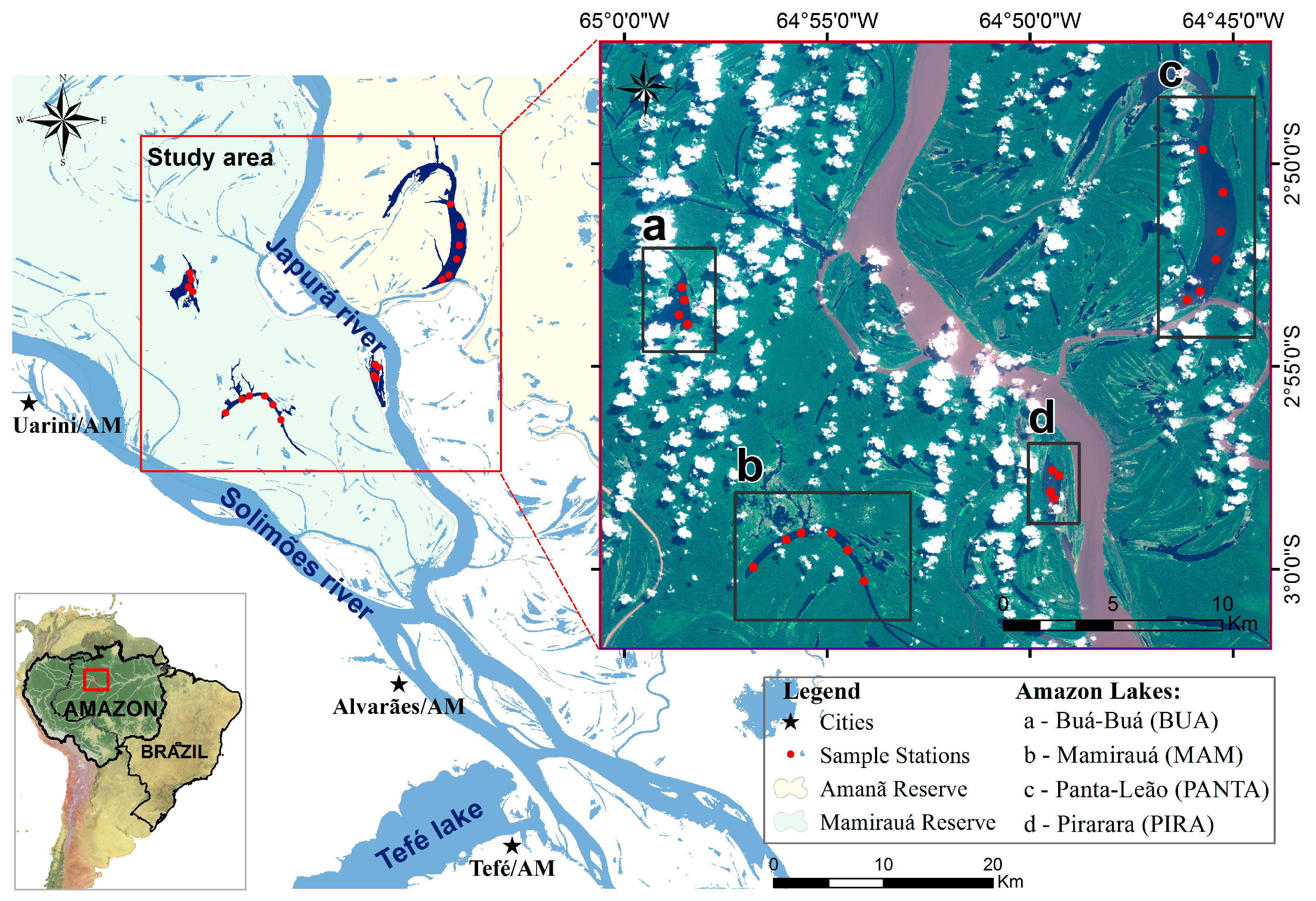
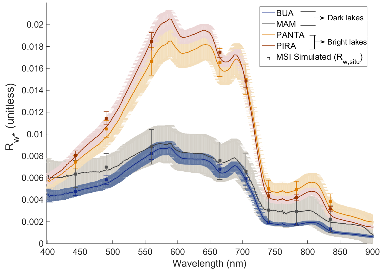
2.1. Site Description and Field Data
2.2. MSI/Sentinel-2 Data
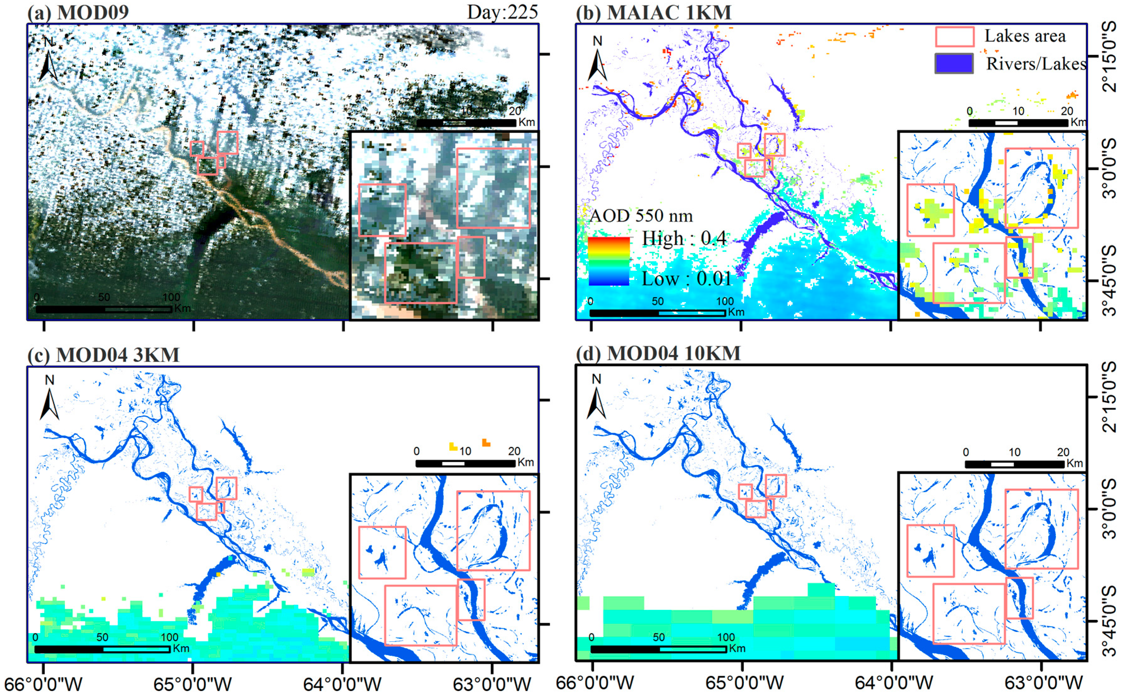
2.3. MAIAC Atmospheric Data
3. Methods
3.1. 6SV Model + MAIAC Atmospheric Products
3.2. ACOLITE Algorithm
3.3. Sen2Cor Algorithm
3.4. Adjacency Effect Correction
4. Results and Discussion
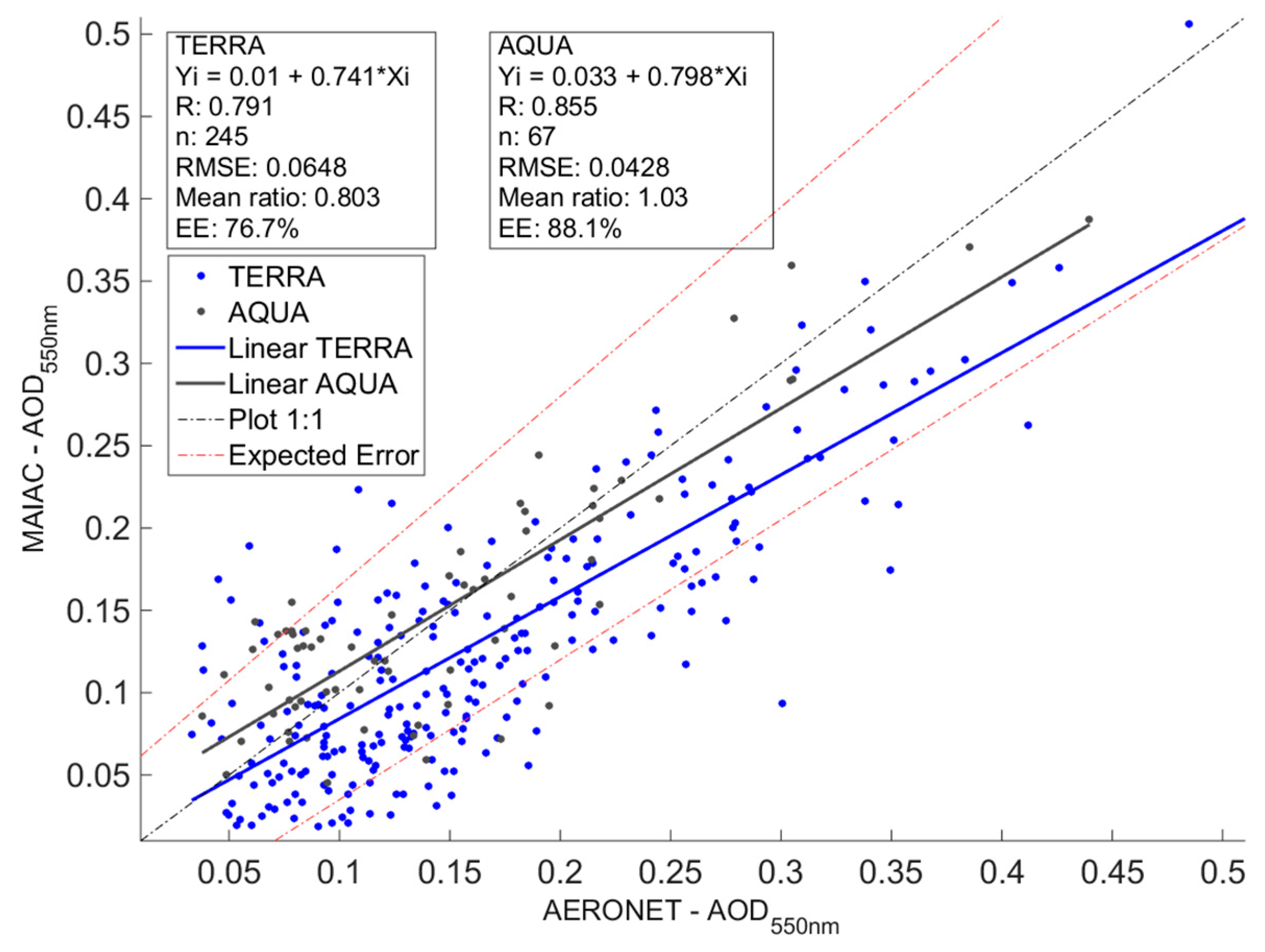
4.1. Evaluation of MAIAC AOD550
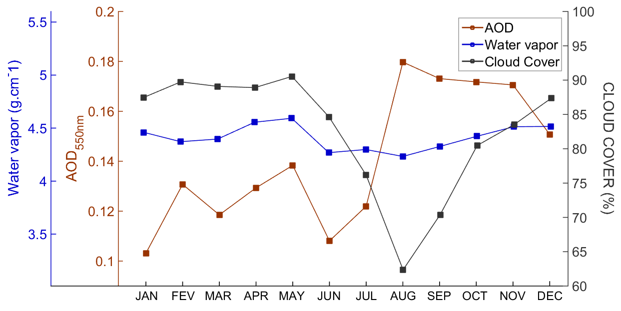
4.2. Background of Atmospheric Constituents
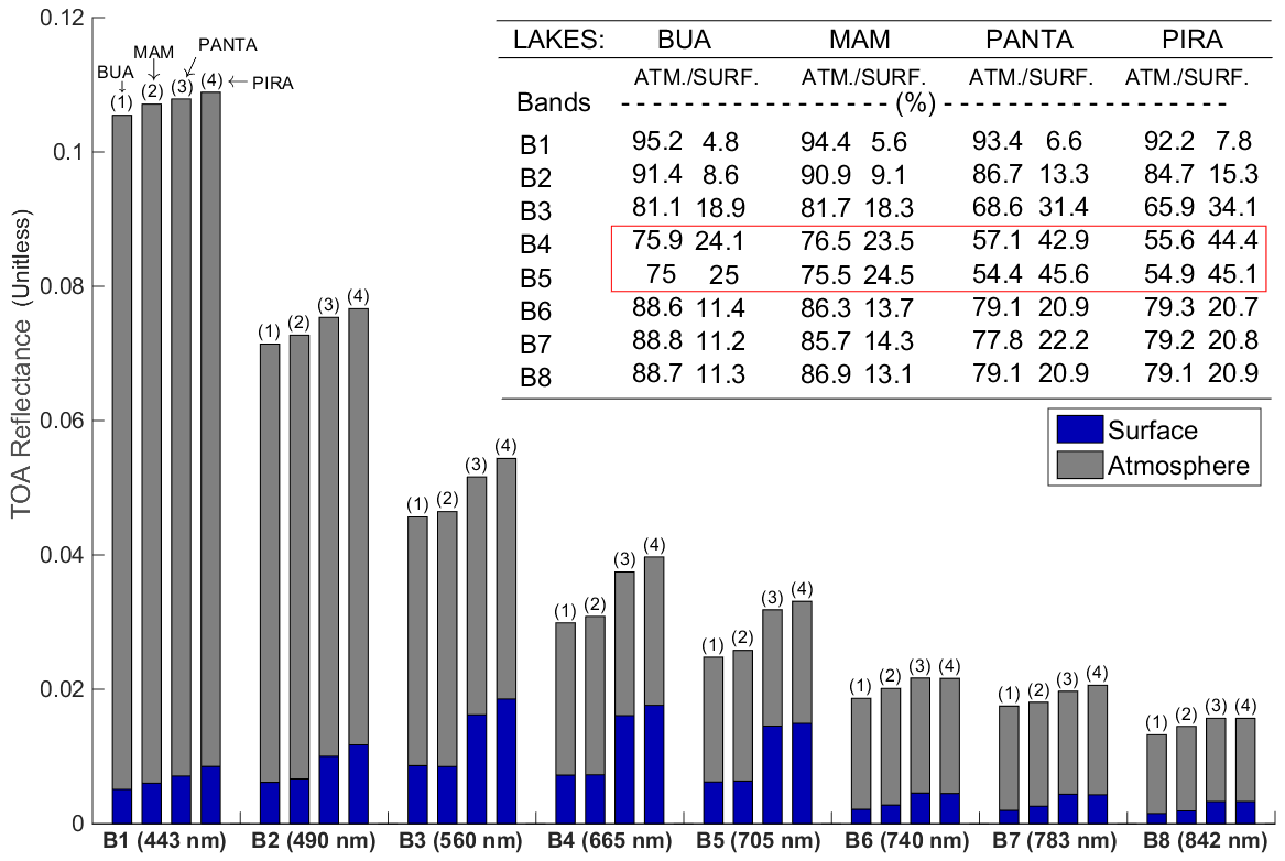
4.3. TOA Simulation Analysis
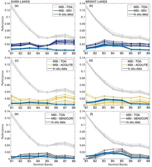
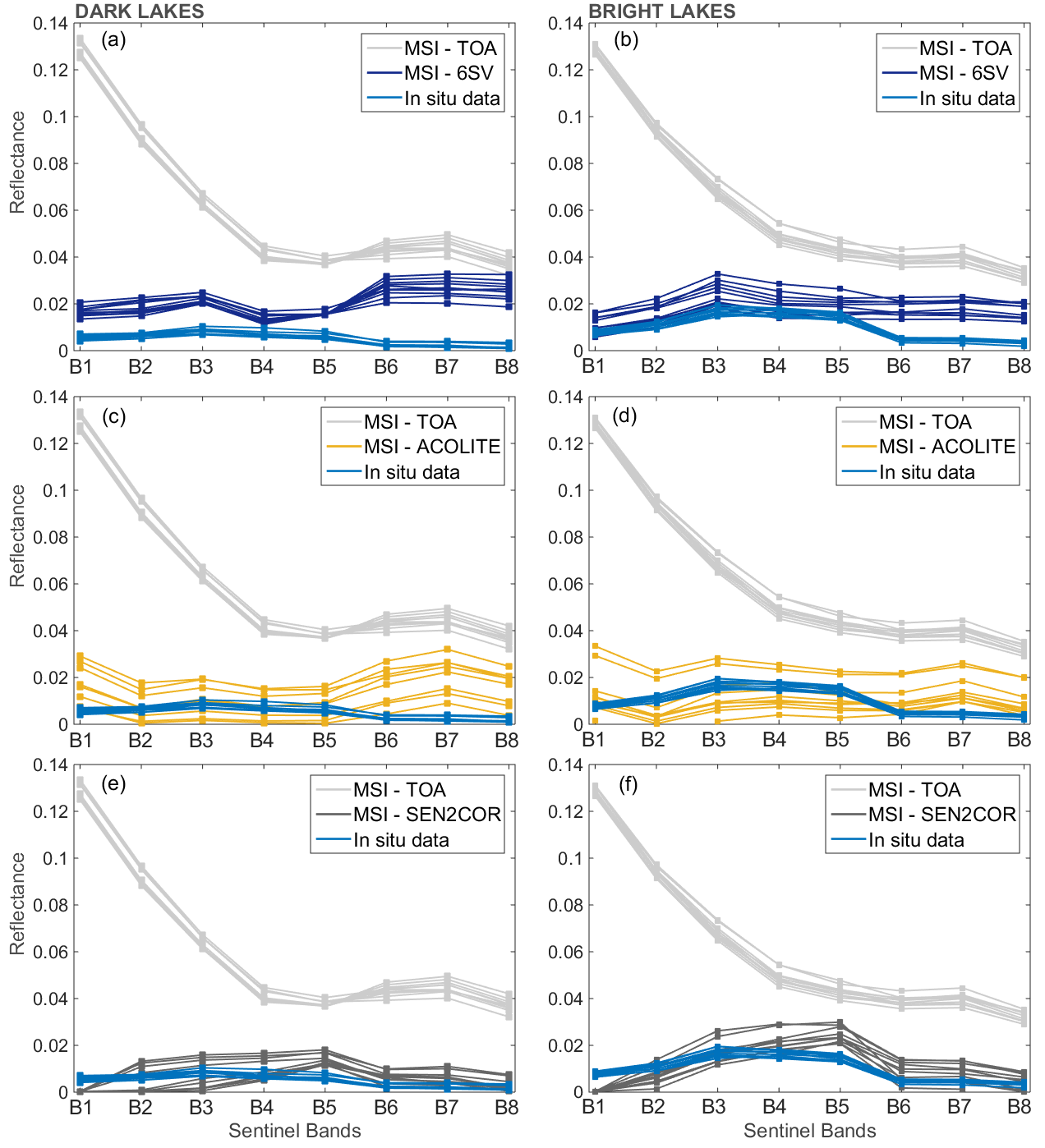
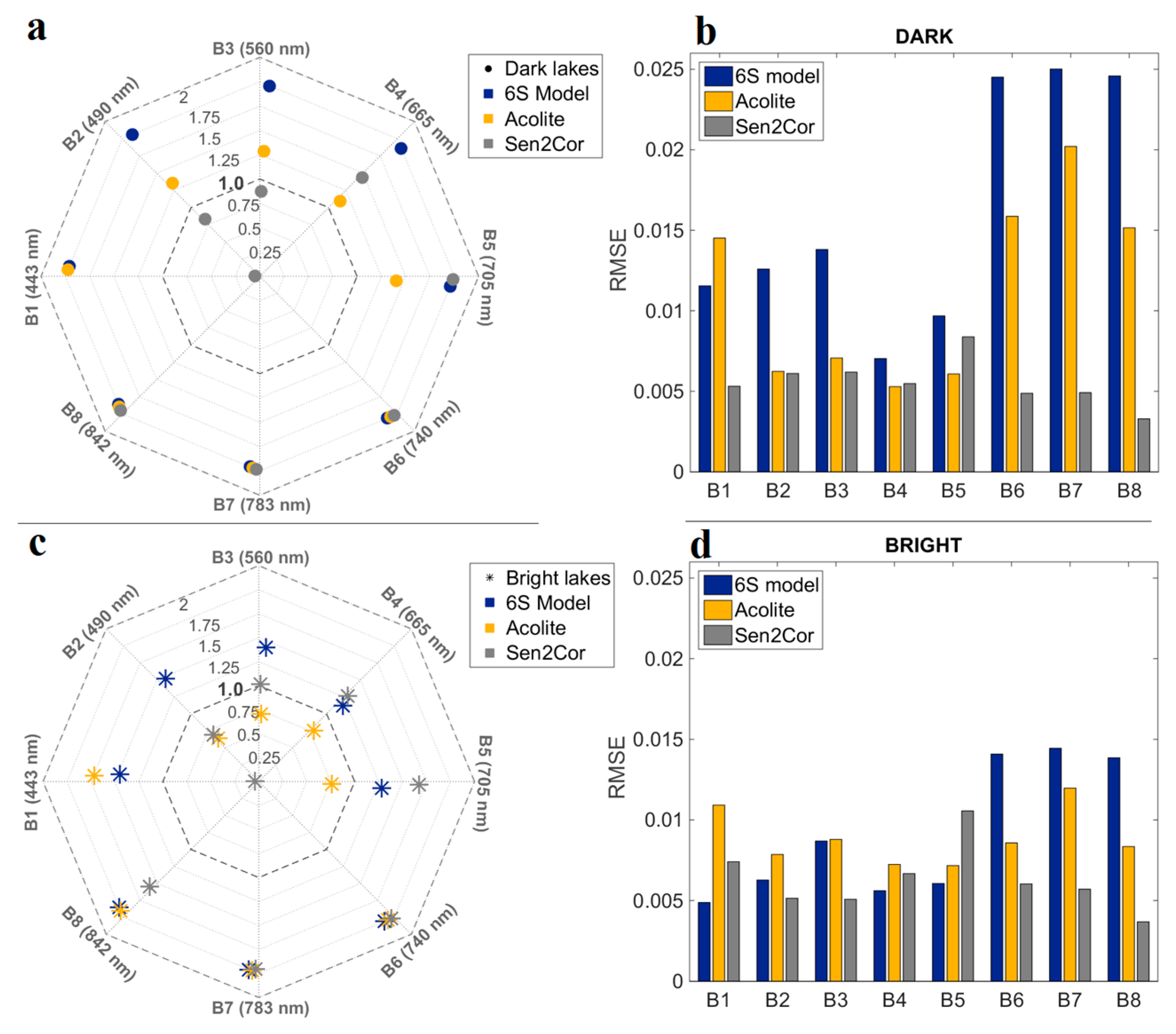
4.4. Inter-Comparison of Atmospheric Correction Methods
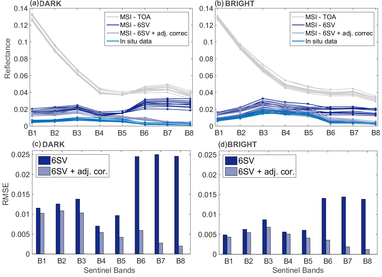
4.5. Adjacency Effect Correction
5. Conclusions
Acknowledgments
Author Contributions
Conflicts of Interest
References
- Dudgeon, D.; Arthington, A.H.; Gessner, M.O.; Kawabata, Z.-I.; Knowler, D.J.; Lévêque, C.; Naiman, R.J.; Prieur-Richard, A.-H.; Soto, D.; Stiassny, M.L.J.; et al. Freshwater biodiversity: Importance, threats, status and conservation challenges. Biol. Rev. 2006, 81, 163–182. [Google Scholar] [PubMed]
- Vörösmarty, C.J.; McIntyre, P.B.; Gessner, M.O.; Dudgeon, D.; Prusevich, A.; Green, P.; Glidden, S.; Bunn, S.E.; Sullivan, C.A.; Liermann, C.R.; et al. Global threats to human water security and river biodiversity. Nature 2010, 467, 555–561. [Google Scholar] [CrossRef] [PubMed]
- Abell, R.; Thieme, M.L.; Revenga, C.; Bryer, M.; Kottelat, M.; Bogutskaya, N.; Coad, B.; Mandrak, N.; Balderas, S.C.; Bussing, W.; et al. Freshwater ecoregions of the world: A new map of biogeographic units for freshwater biodiversity conservation. Bioscience 2008, 58, 403–414. [Google Scholar] [CrossRef]
- Mertes, L.; Smith, M.; Adams, J. Estimating suspended sediment concentrations in surface waters of the Amazon River wetlands from Landsat images. Remote Sens. Environ. 1993, 43, 281–301. [Google Scholar] [CrossRef]
- Park, E.; Latrubesse, E.M. Modeling suspended sediment distribution patterns of the Amazon River using MODIS data. Remote Sens. Environ. 2014, 147, 232–242. [Google Scholar] [CrossRef]
- Lobo, F.L.; Costa, M.P.F.; Novo, E.M.L.M. Time-series analysis of Landsat-MSS/TM/OLI images over Amazonian waters impacted by gold mining activities. Remote Sens. Environ. 2014, 157, 170–184. [Google Scholar] [CrossRef]
- Espinoza Villar, R.; Martinez, J.M.; Guyot, J.L.; Fraizy, P.; Armijos, E.; Crave, A.; Bazán, H.; Vauchel, P.; Lavado, W. The integration of field measurements and satellite observations to determine river solid loads in poorly monitored basins. J. Hydrol. 2012, 444, 221–228. [Google Scholar] [CrossRef]
- Bukata, R.P.; Jerome, J.H.; Kondratyev, A.S.; Pozdnyakov, D.V. Optical Properties and Remote Sensing of Inland and Coastal Waters; CRC Press: Boca Raton, FL, USA, 1995. [Google Scholar]
- Palmer, S.C.J.; Kutser, T.; Hunter, P.D. Remote sensing of inland waters: Challenges, progress and future directions. Remote Sens. Environ. 2015, 157, 1–8. [Google Scholar] [CrossRef]
- Drusch, M.; Del Bello, U.; Carlier, S.; Colin, O.; Fernandez, V.; Gascon, F.; Hoersch, B.; Isola, C.; Laberinti, P.; Martimort, P.; et al. Sentinel-2: ESA’s Optical High-Resolution Mission for GMES Operational Services. Remote Sens. Environ. 2012, 120, 25–36. [Google Scholar] [CrossRef]
- Dörnhöfer, K.; Göritz, A.; Gege, P.; Pflug, B.; Oppelt, N. Water Constituents and Water Depth Retrieval from Sentinel-2A—A First Evaluation in an Oligotrophic Lake. Remote Sens. 2016, 8, 941. [Google Scholar] [CrossRef]
- Toming, K.; Kutser, T.; Laas, A.; Sepp, M.; Paavel, B.; Nõges, T. First Experiences in Mapping Lake Water Quality Parameters with Sentinel-2 MSI Imagery. Remote Sens. 2016, 8, 640. [Google Scholar] [CrossRef]
- Hedley, J.; Roelfsema, C.; Koetz, B.; Phinn, S. Capability of the Sentinel 2 mission for tropical coral reef mapping and coral bleaching detection. Remote Sens. Environ. 2012, 120, 145–155. [Google Scholar] [CrossRef]
- Malthus, T.J.; Hestir, E.L.; Dekker, A.G.; Brando, V.E. The case for a global inland water quality product. In Proceedings of the 2012 IEEE International Geoscience and Remote Sensing Symposium, Munich, Germany, 22–27 July 2012; pp. 5234–5237. [Google Scholar]
- Malenovský, Z.; Rott, H.; Cihlar, J.; Schaepman, M.E.; García-Santos, G.; Fernandes, R.; Berger, M. Sentinels for science: Potential of Sentinel-1, -2, and -3 missions for scientific observations of ocean, cryosphere, and land. Remote Sens. Environ. 2012, 120, 91–101. [Google Scholar] [CrossRef]
- Gao, B.C.; Montes, M.J.; Davis, C.O.; Goetz, A.F.H. Atmospheric correction algorithms for hyperspectral remote sensing data of land and ocean. Remote Sens. Environ. 2009, 113, S17–S24. [Google Scholar] [CrossRef]
- International Ocean Colour Coorperating Group (IOCCG). Atmospheric Correction for Remotely-Sensed Ocean-Colour Products; International Ocean Colour Coorperating Group (IOCCG): Cape Town, South Africa, 2010. [Google Scholar]
- Okin, G.S.; Gu, J. The impact of atmospheric conditions and instrument noise on atmospheric correction and spectral mixture analysis of multispectral imagery. Remote Sens. Environ. 2015, 164, 130–141. [Google Scholar] [CrossRef]
- Hadjimitsis, D.G.; Clayton, C.R.I.; Hope, V.S. An assessment of the effectiveness of atmospheric correction algorithms through the remote sensing of some reservoirs. Int. J. Remote Sens. 2004, 25, 3651–3674. [Google Scholar] [CrossRef]
- Main-Knorn, M.; Pflug, B.; Debaecker, V.; Louis, J. Calibration and validation plan for the L2A processor and products of the Sentinel-2 Mission. ISPRS Int. Arch. Photogramm. Remote Sens. Spat. Inf. Sci. 2015, 40, 1249–1255. [Google Scholar] [CrossRef]
- Vanhellemont, Q.; Ruddick, K. Acolite for Sentinel-2: Aquatic applications of MSI imagery. In Proceedings of the ESA Living Planet Symposium, Pragur, Czech Republic, 9–13 May 2016. [Google Scholar]
- Shi, W.; Wang, M. An assessment of the black ocean pixel assumption for MODIS SWIR bands. Remote Sens. Environ. 2009, 113, 1587–1597. [Google Scholar] [CrossRef]
- Vermote, E.F.; Tanré, D.; Deuzé, J.L.; Herman, M.; Morcrette, J.J. Second simulation of the satellite signal in the solar spectrum, 6S: An overview. IEEE Trans. Geosci. Remote Sens. 1997, 35, 675–686. [Google Scholar]
- Taylor, M.; Kazadzis, S.; Amiridis, V.; Kahn, R.A. Global aerosol mixtures and their multiyear and seasonal characteristics. Atmos. Environ. 2015, 116, 112–129. [Google Scholar] [CrossRef]
- Holben, B.N.; Eck, T.F.; Slutsker, I.; Tanré, D.; Buis, J.P.; Setzer, A.; Vermote, E.; Reagan, J.A.; Kaufman, Y.J.; Nakajima, T.; et al. AERONET—A federated instrument network and data archive for aerosol characterization. Remote Sens. Environ. 1998, 66, 1–16. [Google Scholar] [CrossRef]
- King, M.D.; Menzel, W.P.; Kaufman, Y.J.; Tanre, D.; Gao, B.-C.; Platnick, S.; Ackerman, S.A.; Remer, L.A.; Pincus, R.; Hubanks, P.A. Cloud and aerosol properties, precipitable water, and profiles of temperature and water vapor from MODIS. IEEE Trans. Geosci. Remote Sens. 2003, 41, 442–458. [Google Scholar] [CrossRef]
- Lyapustin, A.; Wang, Y.; Laszlo, I.; Kahn, R.; Korkin, S.; Remer, L.; Levy, R.; Reid, J.S. Multiangle implementation of atmospheric correction (MAIAC): 2. Aerosol algorithm. J. Geophys. Res. Atmos. 2011, 116, 1–15. [Google Scholar] [CrossRef]
- Hilker, T.; Lyapustin, A.I.; Tucker, C.J.; Sellers, P.J.; Hall, F.G.; Wang, Y. Remote sensing of tropical ecosystems: Atmospheric correction and cloud masking matter. Remote Sens. Environ. 2012, 127, 370–384. [Google Scholar] [CrossRef]
- Kiselev, V.; Bulgarelli, B.; Heege, T. Sensor independent adjacency correction algorithm for coastal and inland water systems. Remote Sens. Environ. 2015, 157, 85–95. [Google Scholar] [CrossRef]
- Sterckx, S.; Knaeps, S.; Kratzer, S.; Ruddick, K. SIMilarity Environment Correction (SIMEC) applied to MERIS data over inland and coastal waters. Remote Sens. Environ. 2015, 157, 96–110. [Google Scholar] [CrossRef]
- Ramalho, E.E.; Macedo, J.; Vieira, T.M.; Valsecchi, J.; Calvimontes, J.; Marmontel, M.; Queiroz, H.L. Ciclo hidrológico nos ambientes de várzea. Uakari 2009, 5, 61–87. [Google Scholar]
- Affonso, A.G.; Queiroz, H.L.; Novo, E.M.L.M. Abiotic variability among different aquatic systems of the central Amazon floodplain during drought and flood events. Braz. J. Biol. 2015, 75, 60–69. [Google Scholar]
- Affonso, A.G.; Queiroz, H.L.; De Novo, E.M.L.d.M. Limnological characterization of floodplain lakes in Mamirauá Sustainable Development Reserve, Central Amazon (Amazonas State, Brazil). Acta Limnol. Bras. 2011, 23, 95–108. [Google Scholar] [CrossRef]
- Henderson, P.A.; Hamilton, W.D.; Crampton, W.G.R. Evolution and Diversity in Amazonian Floodplain Communities. In Dynamics of Tropical Communities: 37th Symposium of the British Ecological Society; Cambridge University Press: Cambridge, UK, 1998; pp. 384–398. [Google Scholar]
- Maccord, P.F.L.; Silvano, R.A.M.; Ramires, M.S.; Clauzet, M.; Begossi, A. Dynamics of artisanal fisheries in two Brazilian Amazonian reserves: Implications to co-management. Hydrobiologia 2007, 583, 365–376. [Google Scholar] [CrossRef]
- Castello, L.; Viana, J.P.; Watkins, G.; Pinedo-Vasquez, M.; Luzadis, V.A. Lessons from Integrating Fishers of Arapaima in Small-Scale Fisheries Management at the Mamirauá Reserve, Amazon. Environ. Manag. 2009, 43, 197–209. [Google Scholar] [CrossRef] [PubMed]
- Mobley, C.D. Estimation of the Remote-Sensing Reflectance from Above-Surface Measurements. Appl. Opt. 1999, 38, 7442. [Google Scholar] [CrossRef] [PubMed]
- Mobley, C.D. Polarized reflectance and transmittance properties of windblown sea surfaces. Appl. Opt. 2015, 54, 4828. [Google Scholar] [PubMed]
- Gascon, F.; Cadau, E.; Colin, O.; Hoersch, B.; Isola, C.; López Fernández, B.; Martimort, P. Copernicus Sentinel-2 mission: Products, algorithms and Cal/Val. Proc. SPIE 2014. [Google Scholar] [CrossRef]
- Clevers, J.G.P.W.; Gitelson, A.A. Remote estimation of crop and grass chlorophyll and nitrogen content using red-edge bands on Sentinel-2 and -3. Int. J. Appl. Earth Obs. Geoinf. 2013, 23, 344–351. [Google Scholar] [CrossRef]
- Baillarin, S.J.; Meygret, A.; Dechoz, C.; Petrucci, B.; Lacherade, S.; Tremas, T.; Isola, C.; Martimort, P.; Spoto, F. Sentinel-2 level 1 products and image processing performances. In Proceedings of the 2012 IEEE International Geoscience and Remote Sensing Symposium, Munich, Germany, 22–27 July 2012; pp. 7003–7006. [Google Scholar]
- Kloiber, S.M.; Brezonik, P.L.; Olmanson, L.G.; Bauer, M.E. A procedure for regional lake water clarity assessment using Landsat multispectral data. Remote Sens. Environ. 2002, 82, 38–47. [Google Scholar]
- Olmanson, L.G.; Bauer, M.E.; Brezonik, P.L. A 20-year Landsat water clarity census of Minnesota’s 10,000 lakes. Remote Sens. Environ. 2008, 112, 4086–4097. [Google Scholar] [CrossRef]
- Sriwongsitanon, N.; Surakit, K.; Thianpopirug, S. Influence of atmospheric correction and number of sampling points on the accuracy of water clarity assessment using remote sensing application. J. Hydrol. 2011, 401, 203–220. [Google Scholar] [CrossRef]
- Tebbs, E.J.; Remedios, J.J.; Harper, D.M. Remote sensing of chlorophyll-a as a measure of cyanobacterial biomass in Lake Bogoria, a hypertrophic, saline–alkaline, flamingo lake, using Landsat ETM+. Remote Sens. Environ. 2013, 135, 92–106. [Google Scholar] [CrossRef]
- Remer, L.A.; Kaufman, Y.J.; Tanré, D.; Mattoo, S.; Chu, D.A.; Martins, J.V.; Li, R.-R.; Ichoku, C.; Levy, R.C.; Kleidman, R.G.; et al. The MODIS Aerosol Algorithm, Products, and Validation. J. Atmos. Sci. 2005, 62, 947–973. [Google Scholar] [CrossRef]
- Gao, B.-C.; Kaufman, Y.J. Water vapor retrievals using Moderate Resolution Imaging Spectroradiometer (MODIS) near-infrared channels. J. Geophys. Res. Atmos. 2003. [Google Scholar] [CrossRef]
- Hubanks, P.; Platnick, S.; King, M. MODIS Atmosphere L3 Gridded Product Algorithm Theoretical Basis Document (ATBD); Users Guide, ATBDMOD-30; NASA: Greenbelt, MD, USA, 2015.
- Jiménez-Muñoz, J.C.; Sobrino, J.A.; Mattar, C.; Franch, B. Atmospheric correction of optical imagery from MODIS and Reanalysis atmospheric products. Remote Sens. Environ. 2010, 114, 2195–2210. [Google Scholar]
- Lyapustin, A.; Korkin, S.; Wang, Y.; Quayle, B.; Laszlo, I. Discrimination of biomass burning smoke and clouds in MAIAC algorithm. Atmos. Chem. Phys. 2012, 12, 9679–9686. [Google Scholar] [CrossRef]
- Vermote, E.F.; Kotchenova, S. Atmospheric correction for the monitoring of land surfaces. J. Geophys. Res. 2008. [Google Scholar] [CrossRef]
- Vermote, E.; Justice, C.; Claverie, M.; Franch, B. Preliminary analysis of the performance of the Landsat 8/OLI land surface reflectance product. Remote Sens. Environ. 2016, 185, 46–56. [Google Scholar] [CrossRef]
- Kotchenova, S.Y.; Vermote, E.F.; Matarrese, R.; Klemm, F.J., Jr. Validation of a vector version of the 6S radiative transfer code for atmospheric correction of satellite data Part I: Path radiance. Appl. Opt. 2007, 46, 4455–4464. [Google Scholar] [CrossRef] [PubMed]
- Vanhellemont, Q.; Ruddick, K. Turbid wakes associated with offshore wind turbines observed with Landsat 8. Remote Sens. Environ. 2014, 145, 105–115. [Google Scholar] [CrossRef]
- Vanhellemont, Q.; Ruddick, K. Advantages of high quality SWIR bands for ocean colour processing: Examples from Landsat-8. Remote Sens. Environ. 2015, 161, 89–106. [Google Scholar] [CrossRef]
- Pahlevan, N.; Lee, Z.; Wei, J.; Schaaf, C.B.; Schott, J.R.; Berk, A. On-orbit radiometric characterization of OLI (Landsat-8) for applications in aquatic remote sensing. Remote Sens. Environ. 2014, 154, 272–284. [Google Scholar] [CrossRef]
- Franz, B.A.; Bailey, S.W.; Kuring, N.; Werdell, P.J. Ocean Color Measurements from Landsat-8 OLI using SeaDAS. In Proceedings of the Ocean Optics XXII, Portland, MA, USA, 26–31 October 2014; pp. 26–31. [Google Scholar]
- Uwe, M.-W.; Jerome, L.; Rudolf, R.; Ferran, G.; Marc, N. Sentinel-2 Level 2a Prototype Processor: Architecture, Algorithms and First Results. In Proceedings of the ESA Living Planet Symposium, Edinburgh, UK, 9–13 September 2013. [Google Scholar]
- Kaufman, Y.J.; Wald, A.E.; Remer, L.A.; Gao, B.C.; Li, R.-R.; Flynn, L. The MODIS 2.1-μm channel-correlation with visible reflectance for use in remote sensing of aerosol. IEEE Trans. Geosci. Remote Sens. 1997, 35, 1286–1298. [Google Scholar] [CrossRef]
- Tanre, D.; Herman, M.; Deschamps, P.Y. Influence of the background contribution upon space measurements of ground reflectance. Appl. Opt. 1981, 20, 3676–3684. [Google Scholar] [CrossRef] [PubMed]
- Otterman, J.; Fraser, R.S. Adjacency effects on imaging by surface reflection and atmospheric scattering: cross radiance to zenith. Appl. Opt. 1979, 18, 2852–2860. [Google Scholar] [CrossRef] [PubMed]
- Kaufman, Y.J. Atmospheric effect on spatial resolution of surface imagery. Appl. Opt. 1984, 23, 4164–4172. [Google Scholar] [PubMed]
- Chervet, P.; Lavigne, C.; Roblin, A.; Bruscaglioni, P. Effects of aerosol scattering phase function formulation on point-spread-function calculations. Appl. Opt. 2002, 41, 6489–6498. [Google Scholar] [CrossRef] [PubMed]
- Minomura, M.; Kuze, H.; Takeuchi, N. Adjacency effect in the atmospheric correction of satellite remote sensing data: evaluation of the influence of aerosol extinction profiles. Opt. Rev. 2001, 8, 133–141. [Google Scholar] [CrossRef]
- Dor, B.B.; Devir, A.D.; Shaviv, G.; Bruscaglioni, P.; Donelli, P.; Ismaelli, A. Atmospheric scattering effect on spatial resolution of imaging systems. Opt. Soc. Am. 1997, 14, 1329–1337. [Google Scholar]
- Huang, C.; Townshend, J.R.G.; Liang, S.; Kalluri, S.N.V.; Defries, R.S. Impact of sensor’s point spread function on land cover characterization: assessment and deconvolution. Remote Sens. Environ. 2002, 80, 203–212. [Google Scholar] [CrossRef]
- Radoux, J.; Chomé, G.; Jacques, D.C.; Waldner, F.; Bellemans, N.; Matton, N.; Lamarche, C.; D’Andrimont, R.; Defourny, P. Sentinel-2’s Potential for Sub-Pixel Landscape Feature Detection. Remote Sens. 2016, 8, 488. [Google Scholar] [CrossRef]
- Sei, A. Efficient correction of adjacency effects for high- resolution imagery: Integral equations, analytic continuation, and Padé approximants. Appl. Opt. 2015, 54, 3748–3758. [Google Scholar] [CrossRef]
- Duan, S.B.; Li, Z.L.; Tang, B.-H.; Wu, H.; Tang, R.; Bi, Y. Atmospheric correction of high-spatial-resolution satellite images with adjacency effects: Application to EO-1 ALI data. Int. J. Remote Sens. 2015, 36, 5061–5074. [Google Scholar] [CrossRef]
- Vermote, E.F.; El Saleous, N.; Justice, C.O.; Kaufman, Y.J.; Privette, J.L.; Remer, L.; Roger, J.C.; Tanré, D. Atmospheric correction of visible to middle-infrared EOS-MODIS data over land surfaces: Background, operational algorithm and validation. J. Geophys. Res. 1997, 102, 17131–17141. [Google Scholar] [CrossRef]
- Burazerovic, D.; Geens, B.; Heylen, R.; Sterckx, S.; Scheunders, P. Unmixing for detection and quantification of adjacency effects. In Proceedings of the 2012 IEEE International Geoscience and Remote Sensing Symposium, Munich, Germany, 22–27 July 2012; pp. 3090–3093. [Google Scholar]
- Keshava, N.; Mustard, J.F. Spectral unmixing. IEEE Signal Process. Mag. 2002, 19, 44–57. [Google Scholar] [CrossRef]
- Seidel, F.C.; Popp, C. Critical surface albedo and its implications to aerosol remote sensing. Atmos. Meas. Tech. 2012, 5, 1653–1665. [Google Scholar] [CrossRef]
- Remer, L.A.; Tanre, D.; Kaufman, Y.J.; Levy, R.; Mattoo, S. Algorithm for Remote Sensing of Tropospheric Aerosol from MODIS: Collection 005; NASA: Merritt Island, FL, USA, 2006.
- Kondratyev, K.Y.; Kozoderov, V.V.; Smokty, O.I. Remote Sensing of the Earth from Space: Atmospheric Correction; Springer: Berlin, Germany, 2013. [Google Scholar]
- Hilker, T.; Lyapustin, A.I.; Hall, F.G.; Myneni, R.; Knyazikhin, Y.; Wang, Y.; Tucker, C.J.; Sellers, P.J. On the measurability of change in Amazon vegetation from MODIS. Remote Sens. Environ. 2015, 166, 233–242. [Google Scholar]
- Videla, F.C.; Barnaba, F.; Angelini, F.; Cremades, P.; Gobbi, G.P. The relative role of amazonian and non-amazonian fires in building up the aerosol optical depth in South America: A five year study (2005–2009). Atmos. Res. 2013, 122, 298–309. [Google Scholar] [CrossRef]
- Artaxo, P.; Rizzo, L.V.; Brito, J.F.; Barbosa, H.M.J.; Arana, A.; Sena, E.T.; Cirino, G.G.; Bastos, W.; Martin, S.T.; Andreae, M.O. Atmospheric aerosols in Amazonia and land use change: From natural biogenic to biomass burning conditions. Faraday Discuss. 2013, 165, 203–235. [Google Scholar] [CrossRef] [PubMed]
- Bodhaine, B.A.; Wood, N.B.; Dutton, E.G.; Slusser, J.R. On Rayleigh optical depth calculations. J. Atmos. Ocean. Technol. 1999, 16, 1854–1861. [Google Scholar] [CrossRef]
- Kutser, T.; Pierson, D.C.; Kallio, K.Y.; Reinart, A.; Sobek, S. Mapping lake CDOM by satellite remote sensing. Remote Sens. Environ. 2005, 94, 535–540. [Google Scholar] [CrossRef]
- Matthews, M.W. A current review of empirical procedures of remote sensing in inland and near-coastal transitional waters. Int. J. Remote Sens. 2011, 32, 6855–6899. [Google Scholar] [CrossRef]
- Odermatt, D.; Gitelson, A.; Brando, V.E.; Schaepman, M. Review of constituent retrieval in optically deep and complex waters from satellite imagery. Remote Sens. Environ. 2012, 118, 116–126. [Google Scholar] [CrossRef]
- Bassani, C.; Manzo, C.; Braga, F.; Bresciani, M.; Giardino, C.; Alberotanza, L. The impact of the microphysical properties of aerosol on the atmospheric correction of hyperspectral data in coastal waters. Atmos. Meas. Tech. 2015, 8, 1593–1604. [Google Scholar] [CrossRef]
- Li, Z.; Zhao, X.; Kahn, R.; Mishchenko, M.; Remer, L.; Lee, K.-H.; Wang, M.; Laszlo, I.; Nakajima, T.; Maring, H. Uncertainties in satellite remote sensing of aerosols and impact on monitoring its long-term trend: A review and perspective. Ann. Geophys. 2009, 27, 2755–2770. [Google Scholar] [CrossRef]
- Eck, T.F.; Holben, B.N.; Reid, J.S.; Dubovik, O.; Smirnov, A.; O’Neill, N.T.; Slutsker, I.; Kinne, S. Wavelength dependence of the optical depth of biomass burning, urban, and desert dust aerosols. J. Geophys. Res. 1999, 104, 31333–31349. [Google Scholar]
- Barnes, B.B.; Hu, C.; Kovach, C.; Silverstein, R.N. Sediment plumes induced by the Port of Miami dredging: Analysis and interpretation using Landsat and MODIS data. Remote Sens. Environ. 2015, 170, 328–339. [Google Scholar] [CrossRef]
- Garaba, S.P.; Zielinski, O. An assessment of water quality monitoring tools in an estuarine system. Remote Sens. Appl. Soc. Environ. 2015, 2, 1–10. [Google Scholar] [CrossRef]
- Louis, J.; Debaecker, V.; Pflug, B.; Main-Knorn, M. Sentinel-2 Sen2Cor: L2A Processor for Users. In Proceedings of the Living Planet Symposium, Prague, Czech Republic, 9–13 May 2016. [Google Scholar]
- Wilson, R.T. Py6S: A Python interface to the 6S radiative transfer model. Comput. Geosci. 2013, 51, 166–171. [Google Scholar] [CrossRef]


| MSI Bands (Spatial Resolution) | Central Wavelength (nm) | Bandwidth (nm) | Lref (W·m−2·sr−1·μm−1) | SNR at Lref |
|---|---|---|---|---|
| Band 1 (60 m) | 443 (Deep blue) | 20 | 129 | 129 |
| Band 2 (10 m) | 490 (Blue) | 65 | 128 | 154 |
| Band 3 (10 m) | 560 (Green) | 35 | 128 | 168 |
| Band 4 (10 m) | 665 (Red) | 30 | 108 | 142 |
| Band 5 (20 m) | 705 (Red-edge) | 15 | 74.5 | 117 |
| Band 6 (20 m) | 740 (Red-edge) | 15 | 68 | 89 |
| Band 7 (20 m) | 783 (Red-edge) | 20 | 67 | 105 |
| Band 8 (10 m) | 842 (NIR) | 115 | 103 | 172 |
| Band 8A (20 m) | 865 (NIR) | 20 | 52.5 | 72 |
| Band 9 (60 m) | 945 (NIR) | 20 | 9 | 114 |
| Band 10 (60 m) | 1375 (SWIR) | 30 | 6 | 50 |
| Band 11 (20 m) | 1610 (SWIR) | 90 | 4 | 100 |
| Band 12 (20 m) | 2190 (SWIR) | 180 | 1.5 | 100 |
| Parameters | BUA | MAM | PANTA | PIRA |
|---|---|---|---|---|
| Solar zenith angle (°) | 30.96 | 30.96 | 30.96 | 30.96 |
| Solar azimuth angle (°) | 53.99 | 53.99 | 53.99 | 53.99 |
| Aerosol Model | Biomass Burning | |||
| AOD at 550 nm 1 | 0.3 | 0.26 | 0.34 | 0.3 |
| Ozone (cm-atm) | 0.346 | 0.346 | 0.346 | 0.346 |
| Water vapour (g/cm2) | 4.88 | 4.7 | 4.06 | 4.15 |
| Terrain elevation (km) | 0.04 | 0.04 | 0.04 | 0.04 |
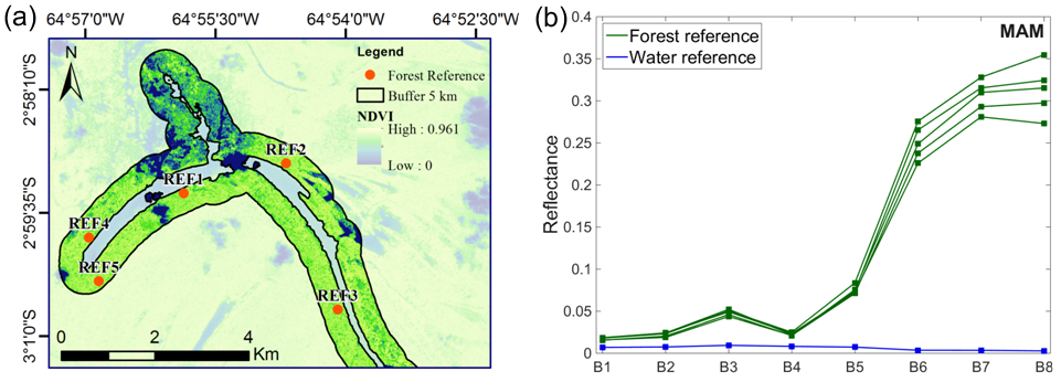
| Lake | Type | B1 | B2 | B3 | B4 | B5 | B6 | B7 | B8 |
|---|---|---|---|---|---|---|---|---|---|
| BUA | Water | 0.005 | 0.006 | 0.008 | 0.007 | 0.006 | 0.002 | 0.002 | 0.002 |
| Forest | 0.023 | 0.031 | 0.062 | 0.030 | 0.096 | 0.289 | 0.341 | 0.343 | |
| MAM | Water | 0.007 | 0.008 | 0.009 | 0.008 | 0.007 | 0.004 | 0.004 | 0.003 |
| Forest | 0.017 | 0.022 | 0.048 | 0.023 | 0.075 | 0.251 | 0.306 | 0.313 | |
| PANTA | Water | 0.008 | 0.011 | 0.017 | 0.017 | 0.016 | 0.006 | 0.006 | 0.005 |
| Forest | 0.009 | 0.015 | 0.042 | 0.019 | 0.072 | 0.249 | 0.300 | 0.296 | |
| PIRA | Water | 0.008 | 0.012 | 0.019 | 0.018 | 0.015 | 0.005 | 0.004 | 0.003 |
| Forest | 0.017 | 0.023 | 0.050 | 0.025 | 0.077 | 0.253 | 0.312 | 0.329 |
© 2017 by the authors. Licensee MDPI, Basel, Switzerland. This article is an open access article distributed under the terms and conditions of the Creative Commons Attribution (CC BY) license (http://creativecommons.org/licenses/by/4.0/).
Share and Cite
Martins, V.S.; Barbosa, C.C.F.; De Carvalho, L.A.S.; Jorge, D.S.F.; Lobo, F.D.L.; Novo, E.M.L.d.M. Assessment of Atmospheric Correction Methods for Sentinel-2 MSI Images Applied to Amazon Floodplain Lakes. Remote Sens. 2017, 9, 322. https://doi.org/10.3390/rs9040322
Martins VS, Barbosa CCF, De Carvalho LAS, Jorge DSF, Lobo FDL, Novo EMLdM. Assessment of Atmospheric Correction Methods for Sentinel-2 MSI Images Applied to Amazon Floodplain Lakes. Remote Sensing. 2017; 9(4):322. https://doi.org/10.3390/rs9040322
Chicago/Turabian StyleMartins, Vitor Souza, Claudio Clemente Faria Barbosa, Lino Augusto Sander De Carvalho, Daniel Schaffer Ferreira Jorge, Felipe De Lucia Lobo, and Evlyn Márcia Leão de Moraes Novo. 2017. "Assessment of Atmospheric Correction Methods for Sentinel-2 MSI Images Applied to Amazon Floodplain Lakes" Remote Sensing 9, no. 4: 322. https://doi.org/10.3390/rs9040322