Slip Model for the 25 November 2016 Mw 6.6 Aketao Earthquake, Western China, Revealed by Sentinel-1 and ALOS-2 Observations


Abstract
:
1. Introduction
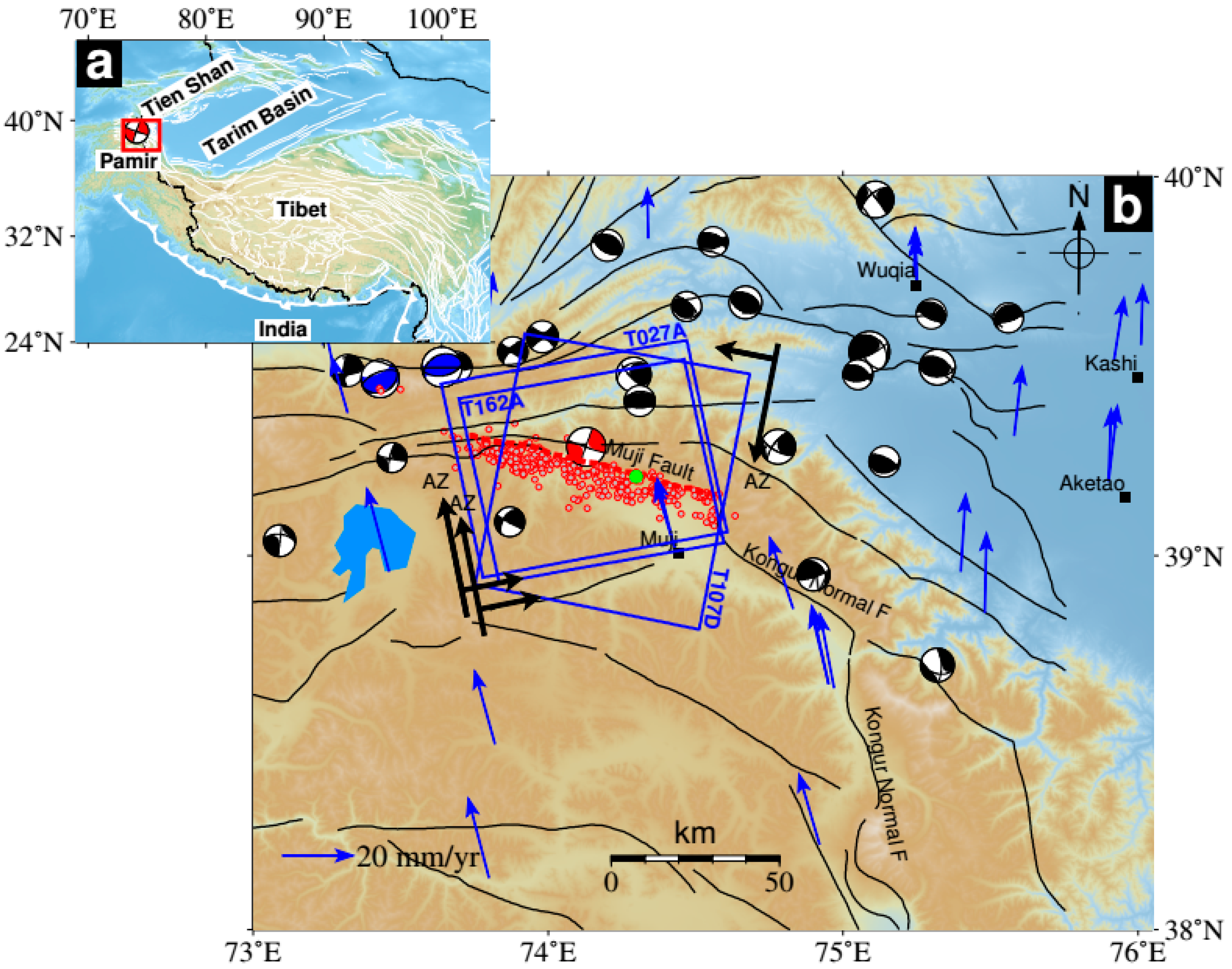
2. Tectonic Setting
3. Coseismic Deformation Mapped by InSAR Observations
3.1. InSAR Observations and Processing
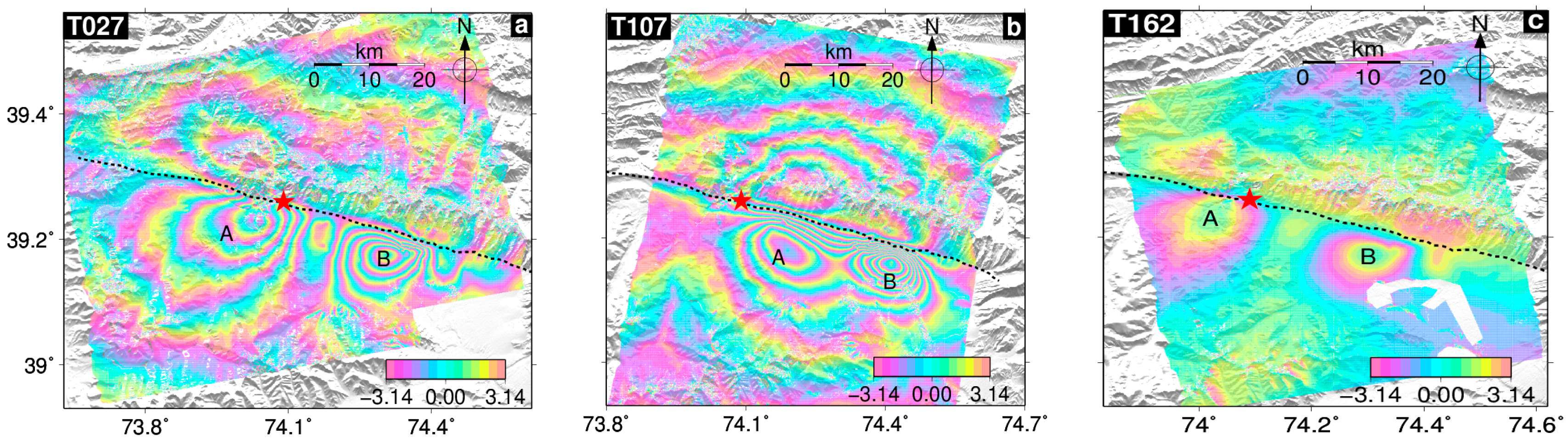
3.2. Coseismic Deformation Mapped by InSAR
4. Finite Slip Model and Static Stress Changes
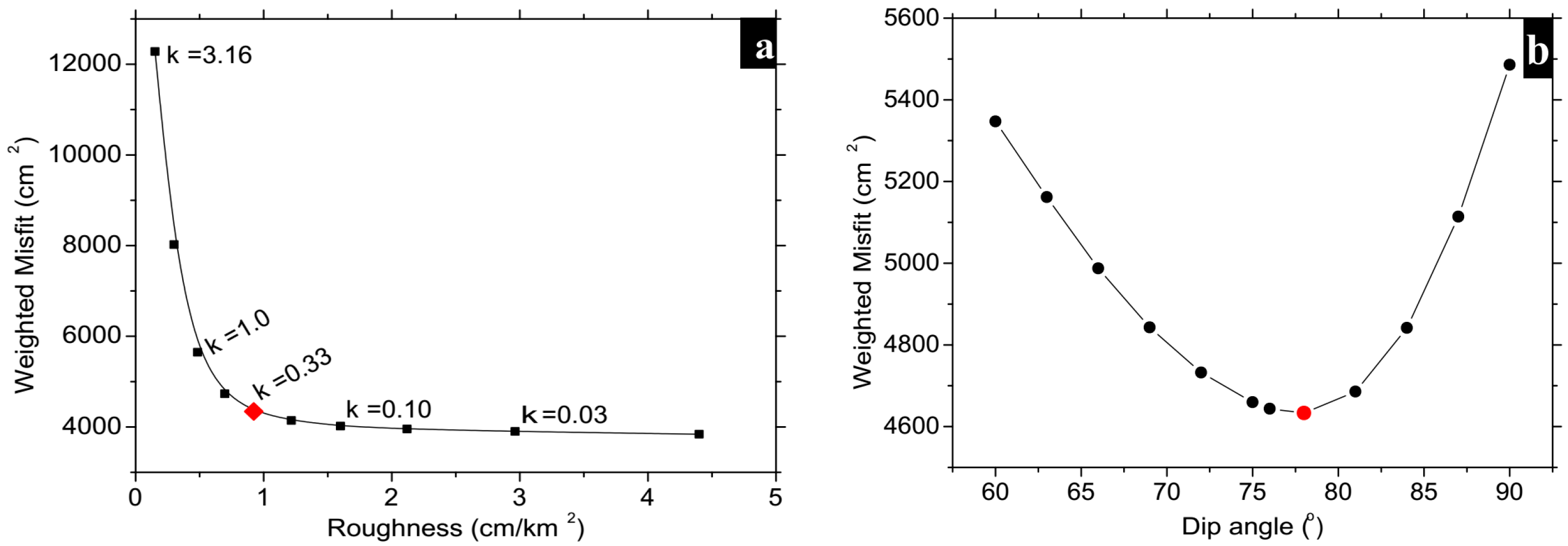
4.1. Methods
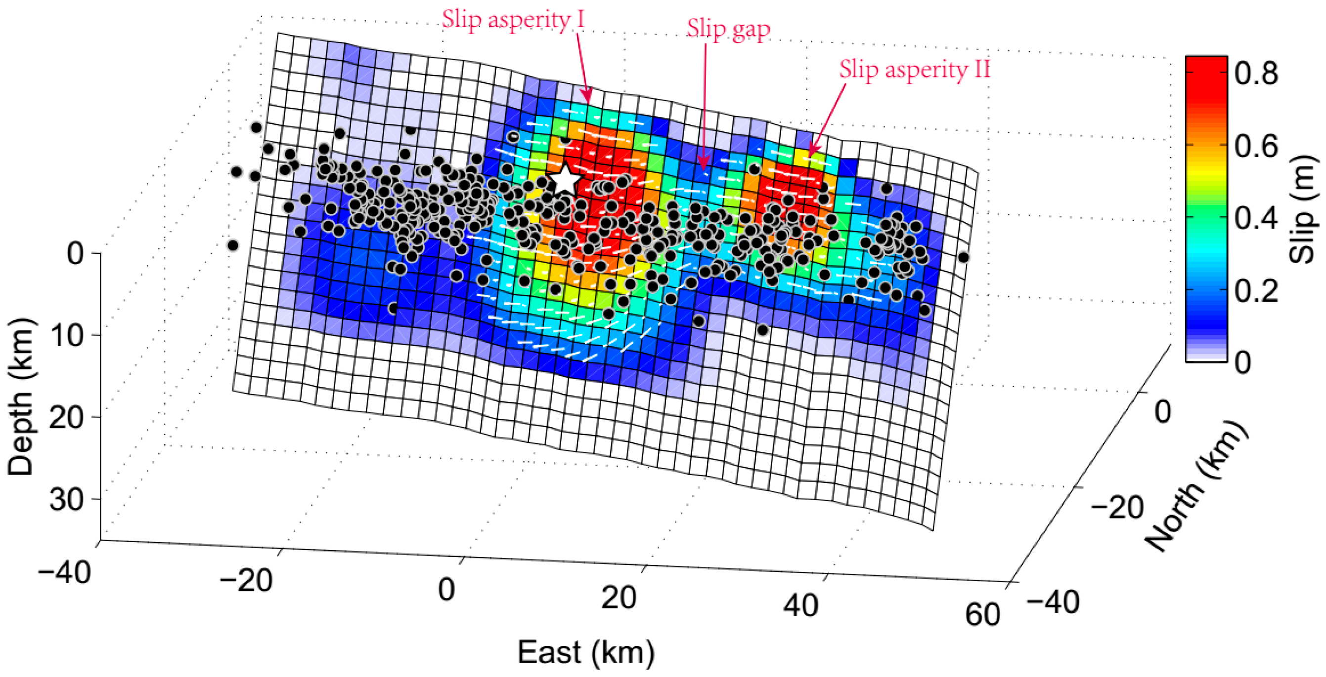
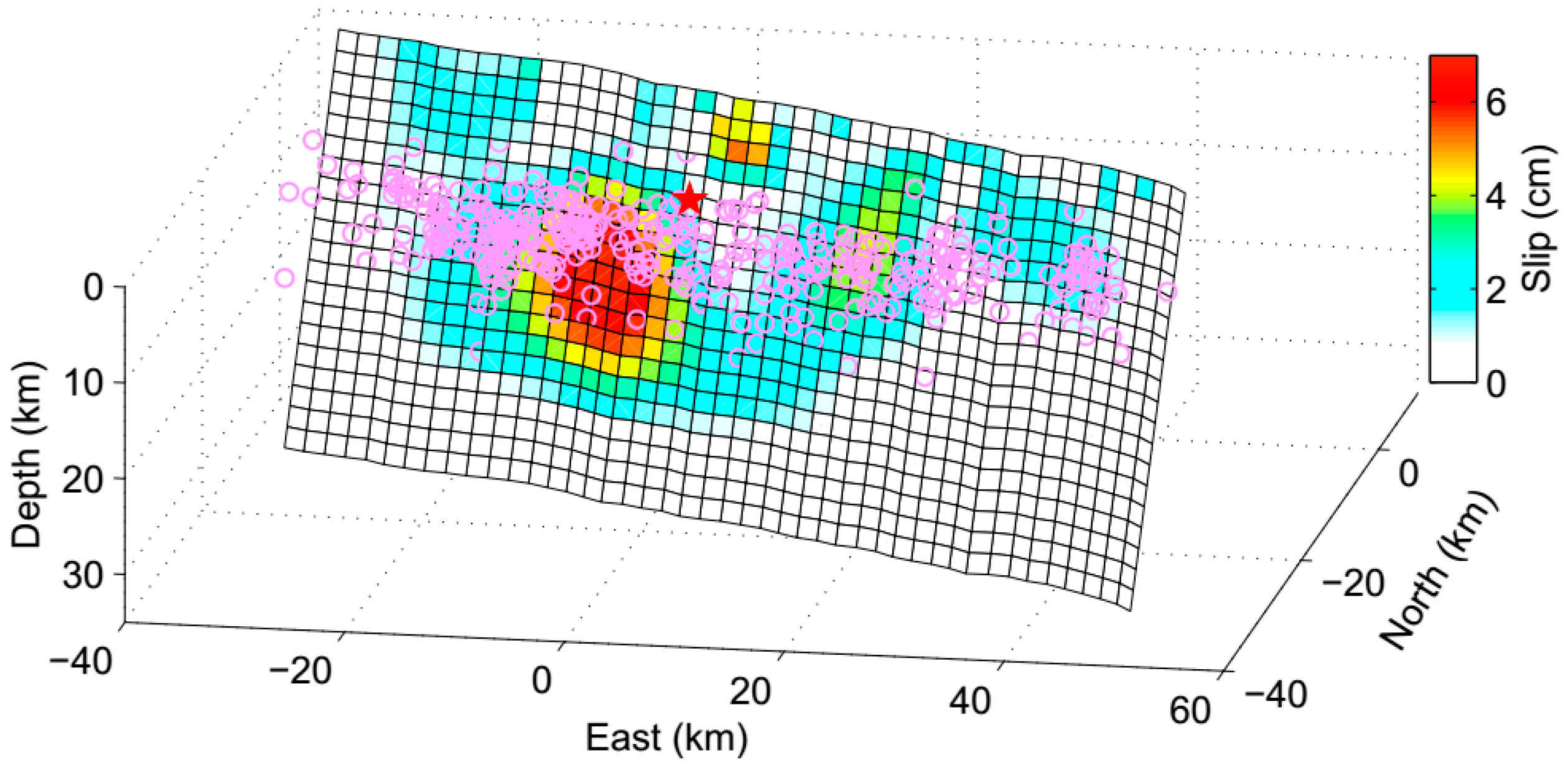
4.2. Finite Slip Model
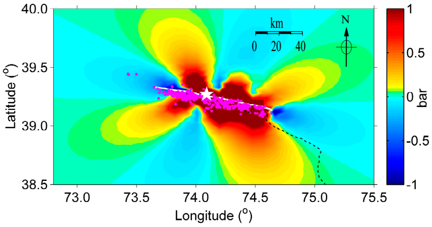
4.3. Static Coulomb Stress Changes
5. Discussion
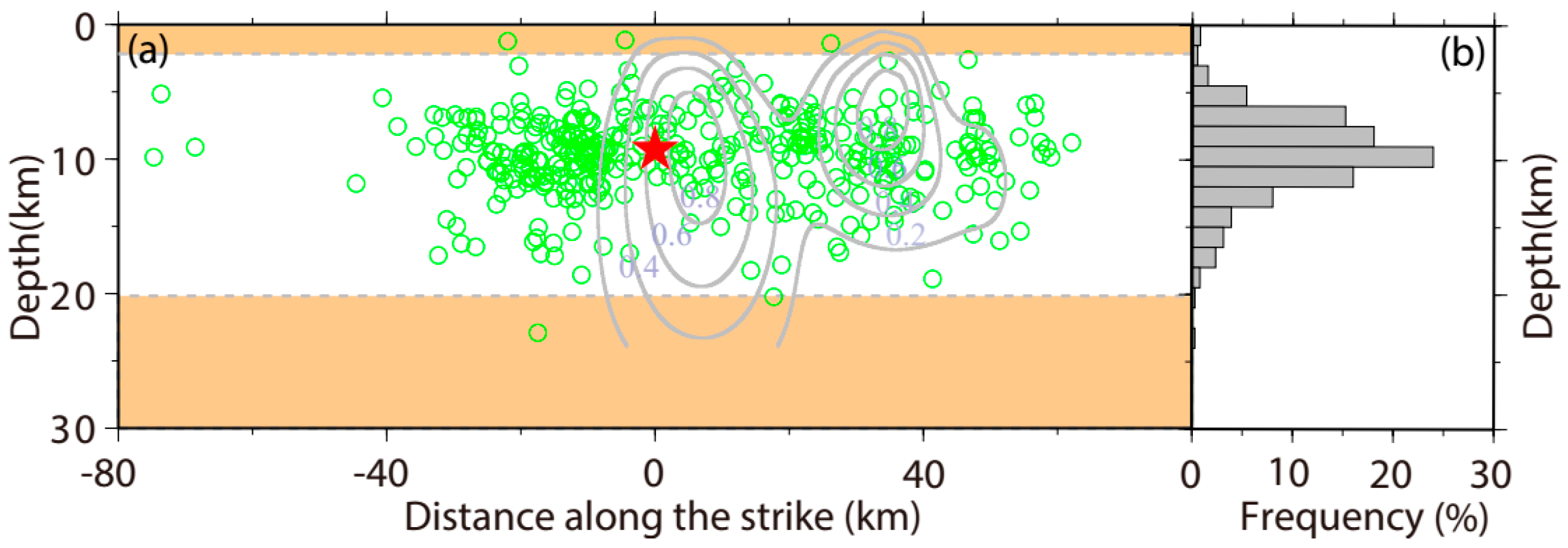
5.1. Implications for the Potential Barrier
5.2. Seismic Energy Source
5.3. Implications of Frictional Properties on the Fault Plane
6. Conclusions
Acknowledgments
Author Contributions
Conflicts of Interest
References
- Chen, J.; Li, T.; Sun, J.B.; Fang, L.H.; Yao, Y.; Li, Y.H.; Wang, H.R.; Fu, B. Coseismic surface rupture and seismogenic Muji fault of the 25 November 2016 Aketao Mw 6.6 earthquake in northern Pamir. Seismol. Geol. 2016, 38, 1160–1174. [Google Scholar]
- Fang, L.; Wu, J.; Wang, W.; Du, W.; Su, J.; Wang, C.; Yang, T.; Cai, Y. Aftershock observation and analysis of the 2013 Ms 7.0 Lushan earthquake. Seismol. Res. Lett. 2015, 86, 1135. [Google Scholar] [CrossRef]
- USGS. Available online: http://earthquake.usgs.gov/earthquakes/eventpage/us10007ca5#executive (accessed on 26 December 2016).
- GCMT. Available online: http://www.globalcmt.org/ (accessed on 26 December 2016).
- IGP. Available online: http://www.cea-igp.ac.cn/ (accessed on 26 December 2016).
- Wang, W.; Qiao, X.; Yang, S.; Wang, D. Present-day velocity field and block kinematics of Tibetan Plateau from GPS measurements. Geophys. J. Int. 2017, 208, 1088–1102. [Google Scholar] [CrossRef]
- Robinson, A.C.; Yin, A.; Manning, C.E.; Harrison, T.M.; Zhang, S.H.; Wang, X.F. Tectonic evolution of the northeastern Pamir: Constraints from the northern portion of the Cenozoic Kongur Shan extensional system, western China. Geol. Soc. Am. Bull. 2004, 116, 953–973. [Google Scholar] [CrossRef]
- Rutte, D.; Lothar, R.; Schneider, S.; Stübner, K.; Stearns, M.A.; Gulzar, M.A.; Hacker, B.R. Building the Pamir-Tibet Plateau—Crustal Stacking, Extensional Collapse, and Lateral Extrusion in the Central Pamir: 1. Geometry and Kinematics. Tectonics 2017, 36. [Google Scholar] [CrossRef]
- Rutte, D.; Ratschbacher, L.; Khan, J.; Stübner, K.; Hacker, B.R.; Stearns, M.A.; Tichomirowa, M. Building the Pamir-Tibet Plateau-Crustal stacking, Extensional Collapse, and Lateral Extrusion in the Central Pamir: 2. Timing and Rates. Tectonics 2017, 36. [Google Scholar] [CrossRef]
- Okada, Y. Surface deformation due to shear and tensile faults in a half-space. Bull. Seismol. Soc. Am. 1985, 75, 1135–1154. [Google Scholar]
- Schneider, F.M.; Yuan, X.; Schurr, B.; Mechie, J.; Sippl, C.; Haberland, C.; Abdybachaev, U. Seismic imaging of subducting continental lower crust beneath the Pamir. Earth Planet. Sci. Lett. 2013, 375, 101–112. [Google Scholar] [CrossRef]
- Burtman, V.S. Cenozoic crustal shortening between the Pamir and Tien Shan and a reconstruction of the Pamir-Tien Shan transition zone for the Cretaceous and Palaeogene. Tectonophysics 2000, 319, 69–92. [Google Scholar]
- Yin, A.; Harrison, T.M. Geologic evolution of the Himalayan-Tibetan orogen. Annu. Rev. Earth. Planet. Sci. 2000, 28, 211–280. [Google Scholar] [CrossRef]
- Burtman, V.S.; Molnar, P. Geological and geophysical evidence for deep subduction of continental crust beneath the Pamir. Geol. Soc. Am. Spec. Pap. 1993, 281, 1–76. [Google Scholar]
- Beloussov, V.V.; Belyaevsky, N.A.; Borisov, A.A.; Volvovsky, B.S.; Volkovsky, I.S.; Resvoy, D.P.; Marussi, A. Structure of the lithosphere along the deep seismic sounding profile: Tien Shan—Pamirs-Karakorum-Himalayas. Tectonophysics 1980, 70, 193–221. [Google Scholar] [CrossRef]
- Bao, X.; Song, X.; Li, J. High-resolution lithospheric structure beneath Mainland China from ambient noise and earthquake surface-wave tomography. Earth. Planet. Sci. Lett. 2015, 417, 132–141. [Google Scholar] [CrossRef]
- Li, Y.; Gao, M.; Wu, Q. Crustal thickness map of the Chinese mainland from teleseismic receiver functions. Tectonophysics 2014, 611, 51–60. [Google Scholar]
- Zubovich, A.V.; Wang, X.Q.; Scherba, Y.G.; Schelochkov, G.G.; Reilinger, R.; Reigber, C.; Li, J. GPS velocity field for the Tien Shan and surrounding regions. Tectonics 2010, 29. [Google Scholar] [CrossRef]
- Qiao, X.J.; Wang, Q.; Yang, S.M.; Li, J. Study on the focal mechanism and deformation characteristics for the 2008 Mw 6.7 Wuqia earthquake, Xinjiang by InSAR. Chin. J. Geophys. 2014, 57, 1805–1813. [Google Scholar]
- Liu, D.L.; Li, H.B.; Pan, J.W.; Chevalier, M.L.; Pei, J.L.; Sun, Z.M.; Si, J.L.; Xu, W. Morphotectonic study from the northeastern margin of the Pamir to the West Kunlun range and its tectonic implications. Acta Petrol. Sin. 2011, 27, 3499–3512. [Google Scholar]
- Chevalier, M.L.; Li, H.; Pan, J.; Pei, J.; Wu, F.; Xu, W.; Liu, D. Fast slip-rate along the northern end of the Karakorum fault system, western Tibet. Geophys. Res. Lett. 2011, 38. [Google Scholar] [CrossRef]
- Wang, Q.; Zhang, P.Z.; Freymueller, J.T.; Bilham, R.; Larson, K.M.; Lai, X.A.; Liu, J. Present-day crustal deformation in China constrained by global positioning system measurements. Science 2001, 294, 574–577. [Google Scholar] [CrossRef] [PubMed]
- Liu, D.Q.; Liu, M.; Wang, H.T.; Li, J.; Chen, J.; Wang, X.Q. Slip rates and sesmic moment deficits on major faults in the Tianshan region. Chin. J. Geophys. 2016, 59, 1647–1660. [Google Scholar]
- Torres, R.; Snoeij, P.; Geudtner, D.; Bibby, D.; Davidson, M.; Attema, E.; Traver, I.N. GMES Sentinel-1 mission. Remote Sens. Environ. 2012, 120, 9–24. [Google Scholar] [CrossRef]
- Sun, J.; Shen, Z.K.; Li, T.; Chen, J. Thrust faulting and 3D ground deformation of the 3 July 2015 Mw 6.4 Pishan, China earthquake from Sentinel-1A radar interferometry. Tectonophysics 2016, 683, 77–85. [Google Scholar] [CrossRef]
- Wen, Y.; Xu, C.; Liu, Y.; Jiang, G. Deformation and source parameters of the 2015 Mw 6.5 earthquake in Pishan, western China, from Sentinel-1A and ALOS-2 data. Remote Sens. 2016, 8, 134. [Google Scholar] [CrossRef]
- Dai, K.; Li, Z.; Tomás, R.; Liu, G.; Yu, B.; Wang, X.; Stockamp, J. Monitoring activity at the Daguangbao mega-landslide (China) using Sentinel-1 TOPS time series interferometry. Remote Sens. Environ. 2016, 186, 501–513. [Google Scholar] [CrossRef]
- Xu, X.; Sandwell, D.T.; Tymofyeyeva, E.; González-Ortega, A.; Tong, X. Tectonic and anthropogenic deformation at the cerro prieto geothermal step-over revealed by sentinel-1 insar. IEEE Trans. Geosci. Remote Sens. 2017. under review. [Google Scholar]
- ALOS-2. Available online: http://en.alos-pasco.com/alos-2/ (accessed on 26 December 2016).
- Lindsey, E.O.; Natsuaki, R.; Xu, X.; Shimada, M.; Hashimoto, M.; Melgar, D.; Sandwell, D.T. Line-of-sight displacement from ALOS-2 interferometry: Mw 7.8 Gorkha earthquake and Mw 7.3 aftershock. Geophys. Res. Lett. 2015, 42, 6655–6661. [Google Scholar]
- Werner, C.; Wegmüller, U.; Strozzi, T.; Wiesmann, A. GAMMA SAR and interferometric processing software. In Proceedings of the ERS ENVISAT Symposium, Gothenburg, Sweden, 16–20 October 2001. [Google Scholar]
- Yagüe-Martínez, N.; Prats-Iraola, P.; González, F.R.; Brcic, R.; Shau, R.; Geudtner, D.; Bamler, R. Interferometric processing of Sentinel-1 TOPS data. IEEE Trans. Geosci. Remote Sens. 2016, 54, 2220–2234. [Google Scholar] [CrossRef]
- Wegnüller, U.; Werner, C.; Strozzi, T.; Wiesmann, A.; Frey, O.; Santoro, M. Sentinel-1 support in the GAMMA Software. Procedia Comput. Sci. 2016, 100, 1305–1312. [Google Scholar] [CrossRef]
- Farr, T.; Rosen, P.; Caro, E. The shuttle radar topography mission. Rev. Geophys. 2000, 45, 37–55. [Google Scholar]
- Goldstein, R.; Werner, C. Radar interferogram filtering for geophysical applications. Geophys. Res. Lett. 1998, 25, 4035–4038. [Google Scholar] [CrossRef]
- Chen, C.W. Statistical-Cost Network-Flow approaches to two-dimensional phase unwrapping for radar interferometry. Ph.D. Thesis, Stanford University, Stanford, CA, USA, 2001. [Google Scholar]
- Bekaert, D.P.S.; Walters, R.J.; Wright, T.J.; Hooper, A.J.; Parker, D.J. Statistical comparison of InSAR tropospheric correction techniques. Remote Sens. Environ. 2015, 170, 40–47. [Google Scholar] [CrossRef]
- Wright, T.J.; Parsons, B.E.; Lu, Z. Toward mapping surface deformation in three dimensions using InSAR. Geophys. Res. Lett. 2004, 31, L01607.1–L01607.5. [Google Scholar] [CrossRef]
- Fialko, Y.; Sandwell, D.; Agnew, D.; Simons, M.; Shearer, P.; Minster, B. Deformation on nearby faults induced by the 1999 Hector Mine earthquake. Science 2002, 297, 1858–1862. [Google Scholar] [CrossRef] [PubMed]
- Lindsey, E.O.; Fialko, Y.; Bock, Y.; Sandwell, D.T.; Bilham, R. Localized and distributed creep along the southern San Andreas Fault. J. Geophys. Res. 2014, 119, 7909–7922. [Google Scholar]
- Li, T. Active Thrusting and Folding along the Pamir Frontal Thrust System. Ph.D. Thesis, Institute of Geology, China Earthquake Administration, Beijing, China, 2012. [Google Scholar]
- Xu, C.; Liu, Y.; Wen, Y.; Wang, R. Coseismic slip distribution of the 2008 Mw 7.9 Wenchuan earthquake from joint inversion of GPS and InSAR data. Bull. Seismol. Soc. Am. 2010, 100, 2736–2749. [Google Scholar]
- Jiang, G.; Xu, C.; Wen, Y.; Liu, Y.; Yin, Z.; Wang, J. Inversion for coseismic slip distribution of the 2010 Mw 6.9 Yushu Earthquake from InSAR data using angular dislocations. Geophys. J. Int. 2013, 194, 1011–1022. [Google Scholar] [CrossRef]
- Jónsson, S.; Zebker, H.; Segall, P.; Amelung, F. Fault slip distribution of the 1999 Mw 7.1 Hector Mine, California, earthquake, estimated from satellite radar and GPS measurements. Bull. Seismol. Soc. Am. 2002, 92, 1377–1389. [Google Scholar] [CrossRef]
- Lohman, R.B.; Simons, M. Some thoughts on the use of InSAR data to constrain models of surface deformation: Noise structure and data downsampling. Geochem. Geophys. Geosyst. 2005, 6, 359–361. [Google Scholar] [CrossRef]
- Stark, P.B.; Parker, R.L. Bounded-variable least-squares: An algorithm and applications. Comput. Stat. 1995, 10, 129–129. [Google Scholar]
- Parsons, B.; Wright, T.; Rowe, P.; Andrews, J.; Jackson, J.; Walker, R.; Engdahl, E.R. The 1994 Sefidabeh (eastern Iran) earthquakes revisited: New evidence from satellite radar interferometry and carbonate dating about the growth of an active fold above a blind thrust fault. Geophys. J. Int. 2006, 164, 202–217. [Google Scholar]
- Stein, R.S.; Barka, A.A.; Dieterich, J.H. Progressive failure on the North Anatolian fault since 1939 by earthquake stress triggering. Geophys. J. Int. 1997, 128, 594–604. [Google Scholar]
- Toda, S.; Stein, R.S.; Reasenberg, P.A.; Dieterich, J.H.; Yoshida, A. Stress transferred by the 1995 Mw = 6.9 Kobe, Japan, shock: Effect on aftershocks and future earthquake probabilities. J. Geophys. Res. 1998, 103, 24543–24565. [Google Scholar] [CrossRef]
- Xu, C.; Wang, J.; Li, Z.; Drummond, J. Applying the Coulomb failure function with an optimally oriented plane to the 2008 Mw 7.9 Wenchuan earthquake triggering. Tectonophysic. 2010, 491, 119–126. [Google Scholar] [CrossRef]
- Tang, L.L.; Zhao, C.P.; Wang, H.T. Study on the source characteristics of the 2008 Ms 6. 8 Wuqia, Xinjiang earthquake sequence and the stress field on the northeastern boundary of Pamir. Chin. J. Geophys. 2012, 55, 1228–1239. [Google Scholar]
- Jiang, G.; Wen, Y.; Liu, Y.; Xu, X.; Fang, L.; Chen, G.; Xu, C. Joint analysis of the 2014 Kangding, southwest China, earthquake sequence with seismicity relocation and InSAR inversion. Geophys. Res. Lett. 2015, 42, 3273–3281. [Google Scholar] [CrossRef]
- Xu, X.; Tong, X.; Sandwell, D.T.; Milliner, C.W.; Dolan, J.F.; Hollingsworth, J.; Ayoub, F. Refining the shallow slip deficit. Geophys. J. Int. 2016, 204, 1867–1886. [Google Scholar]
- Chen, Y.; Xu, L.; Li, X.; Zhao, M. Source process of the 1990 Gonghe, China, earthquake and tectonic stress field in the Northeastern Qinghai-Xizang (Tibetan) plateau. Pure Appl. Geophys. 1996, 146, 697–715. [Google Scholar]
- Zhang, Y.; Xu, L.S.; Chen, Y.T. Source process of the 2010 Yushu, Qinghai, earthquake. Sci. China Earth Sci. 2010, 53, 1249–1251. [Google Scholar]
- Scholz, C.H. Earthquakes and friction laws. Nature 1998, 391, 37–42. [Google Scholar] [CrossRef]
- Peltzer, G.; Rosen, P.; Rogez, F.; Hudnut, K. Postseismic rebound in fault step-overs caused by pore fluid flow. Science 1996, 273, 1202. [Google Scholar] [CrossRef]
- Hearn, E.H.; Bürgmann, R. The effect of elastic layering on inversions of GPS data for coseismic slip and resulting stress changes: Strike-slip earthquakes. Bull. Seismol. Soc. Am. 2005, 95, 1637–1653. [Google Scholar] [CrossRef]
- Wessel, P.; Smith, W.H. New, improved version of Generic Mapping Tools released. EOS Trans. AGU 1998, 79, 579–579. [Google Scholar] [CrossRef]


| Satellite | Track | Reference Date | Repeat Date | Perp.B * (m) | Mean Coherence | Σ (mm) | λ (km) |
|---|---|---|---|---|---|---|---|
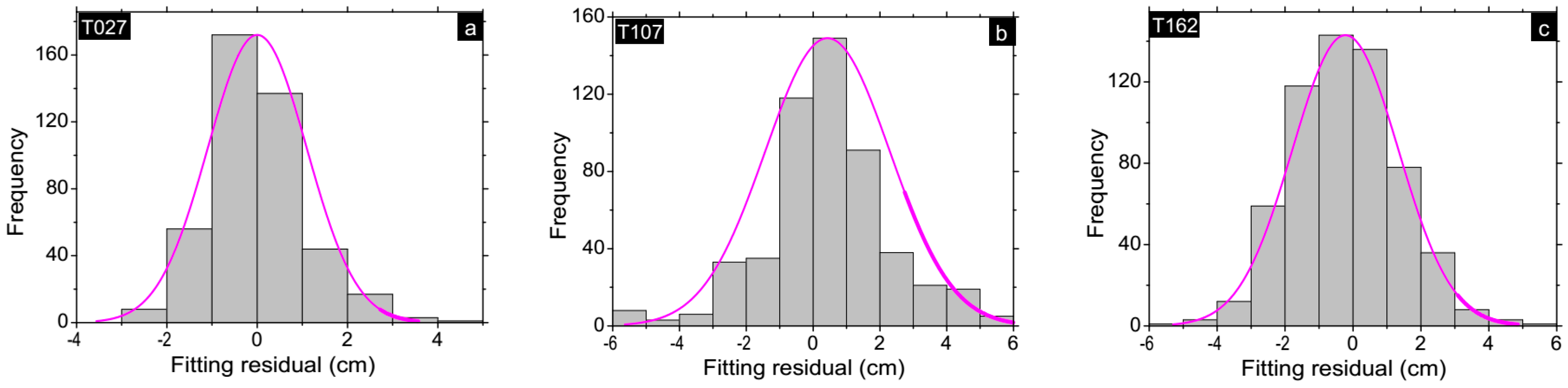
| Sentinel-1A | T027A | 13 November 2016 | 7 December 2016 | −100 | 0.51 | 8.19 | 5.3 |
| Sentinel-1B | T107D | 1 November 2016 | 19 December 2016 | −24 | 0.60 | 9.90 | 9 |
| ALOS-2 | T162A | 20 July 2016 | 7 December 2016 | 92 | 0.77 | 7.00 | 10 |
© 2017 by the authors. Licensee MDPI, Basel, Switzerland. This article is an open access article distributed under the terms and conditions of the Creative Commons Attribution (CC BY) license (http://creativecommons.org/licenses/by/4.0/).
Share and Cite
Wang, S.; Xu, C.; Wen, Y.; Yin, Z.; Jiang, G.; Fang, L. Slip Model for the 25 November 2016 Mw 6.6 Aketao Earthquake, Western China, Revealed by Sentinel-1 and ALOS-2 Observations. Remote Sens. 2017, 9, 325. https://doi.org/10.3390/rs9040325
Wang S, Xu C, Wen Y, Yin Z, Jiang G, Fang L. Slip Model for the 25 November 2016 Mw 6.6 Aketao Earthquake, Western China, Revealed by Sentinel-1 and ALOS-2 Observations. Remote Sensing. 2017; 9(4):325. https://doi.org/10.3390/rs9040325
Chicago/Turabian StyleWang, Shuai, Caijun Xu, Yangmao Wen, Zhi Yin, Guoyan Jiang, and Lihua Fang. 2017. "Slip Model for the 25 November 2016 Mw 6.6 Aketao Earthquake, Western China, Revealed by Sentinel-1 and ALOS-2 Observations" Remote Sensing 9, no. 4: 325. https://doi.org/10.3390/rs9040325