
Seasonal and Interannual Variability of Satellite-Derived Chlorophyll-a (2000–2012) in the Bohai Sea, China


1
School of Marine Sciences, Nanjing University of Information Science & Technology, Nanjing 210044, China
2
Jiangsu Research Centre for Ocean Survey Technology, NUIST, Nanjing 210044, China
*
Author to whom correspondence should be addressed.
Remote Sens. 2017, 9(6), 582; https://doi.org/10.3390/rs9060582
Submission received: 28 February 2017
/
Revised: 5 June 2017
/
Accepted: 5 June 2017
/
Published: 10 June 2017
(This article belongs to the Special Issue Water Optics and Water Colour Remote Sensing)
Abstract
:Knowledge of the chlorophyll-a dynamics and their long-term changes is important for assessing marine ecosystems, especially for coastal waters. In this study, the spatial and temporal variability of sea surface chlorophyll-a concentration (Chl-a) in the Bohai Sea were investigated using 13-year (2000–2012) satellite-derived products from MODIS and SeaWiFS observations. Based on linear regression analysis, the results showed that the entire Bohai Sea experienced an increase in Chl-a on a long-term scale, with the largest increase in the central Bohai Sea and the smallest increase in the Bohai strait. Distinct seasonal patterns of Chl-a existed in different sub-regions of the Bohai Sea. A long-lasting Chl-a peak was observed from May to September in coastal waters (Liaodong bay, Qinhuangdao coast, and Bohai bay) and the central Bohai Sea, whereas Laizhou bay had relatively low Chl-a in early summer. In the Bohai strait, two pronounced Chl-a peaks occurred in March and September, but the lowest Chl-a was in summer. This pattern was quite different from those in other regions of the Bohai Sea. The water column condition (stratified or mixed) was likely an important physical factor that affects the seasonal pattern of Chl-a in the Bohai Sea. Meanwhile, increased human activity (e.g., river discharge) played a significant role in changing the Chl-a distribution in both coastal waters and the central Bohai Sea, especially in summer. The increasing trend of Chl-a in the Bohai Sea might be attributed to the increase in nutrient contents from riverine inputs. The Chl-a dynamics documented in this study provide basic knowledge for the future exploration of marine biogeochemical processes and ecosystem evolution in the Bohai Sea.
1. Introduction
Marine phytoplankton is a fundamental component of marine biogeochemical cycles and ecosystems, accounting for approximately 50% of global organic matter production [1,2]. It also influences the diversity of marine organisms and global climate processes [3,4]. Chlorophyll-a is widely used to indicate phytoplankton biomass [5], as it can generally reflect the situation of phytoplankton growth. Due to the limitation of field methods, chlorophyll-a concentrations (Chl-a) collected by field methods are usually insufficient for investigating the Chl-a dynamics.
Satellite ocean color observations can provide large spatial and temporal coverage, which is ideal for examining the spatial and temporal variability of Chl-a [6]. Empirical and semi-analytical Chl-a algorithms have been developed to infer information about Chl-a from space on both global and regional scales [7,8,9,10]. For instance, the Tassan-like algorithm [8] and OC4 algorithm [10] have been widely applied to satellite data. In addition, the OC4 algorithm was performed on SeaWiFS and MODIS data to derive the NASA standard products of Chl-a, which are provided at http://oceancolour.gsfc.nasa.gov/.
Recent efforts have been made to evaluate Chl-a in the global oceans using satellite-derived products. These studies clearly revealed that increased Chl-a occurred in many coastal waters (e.g., the eastern China seas), and the reason was generally attributed to the interaction between human activity and climate change [11,12,13]. For instance, Gong et al. [14] found that the rate of primary production in the subtropical East China Sea was regulated by seawater temperature during winter and early spring and nutrients during summer and autumn. Shi and Wang [15] studied the seasonal distribution of satellite-derived Chl-a, sea surface temperature (SST), and normalized water leaving radiance (nLw) spectra in the eastern China seas. These results showed that ocean color property variations were driven by the ocean stratification, sea surface thermodynamics, and river discharge, among other factors. Yamaguchi et al. [16] presented the seasonal and summer temporal variability of satellite-derived Chl-a in the Yellow and East China Seas from 1997 to 2007, and revealed that the inter-annual variation of Chl-a in summer was significantly influenced by Yangtze River discharge. He et al. [17] investigated the seasonal and inter-annual variability of phytoplankton blooms in the eastern China seas using satellite-derived Chl-a from 1998 to 2011. They reported that the doubling of the bloom intensity in the eastern China seas was mainly caused by an increase in nitrate and phosphate concentrations. Based on the 15-year (1997–2011) satellite Chl-a data derived using the OC4 algorithm, Liu et al. [18] analyzed the effects of bathymetry on seasonal and inter-annual patterns of Chl-a in a larger region including the Bohai and Yellow Seas, but did not examine the detailed Chl-a dynamics in sub-regions of the Bohai Sea. They also found that the correlation between Chl-a and SST was positive in coastal waters and negative in offshore waters.
Previous researches have commonly investigated the Chl-a dynamics in a large region including the Bohai Sea, such as the studies of He et al. [17] and Liu et al. [18]. However, studies specifically focusing on the Chl-a dynamics on large temporal scales in sub-regions of the Bohai Sea are limited. In addition, the possible factors of Chl-a variation in the Bohai Sea are not yet clear. Because of the highly variable environmental conditions (e.g., river discharge, circulations, and water masses), the Bohai Sea ecosystem is complex [19,20,21]. The phytoplankton growth needs nutrients and light [22]. The available light for photosynthesis depends on photosynthetically available radiation (PAR), extinction coefficient, and water clarity. Additionally, SST may influence the vertical structure of the water column, which would further change the nutrient supply and light conditions. Fortunately, both the SST and PAR parameters can be detected by satellite remote sensing technology, thus providing a large quantity of materials to explore the influences of these two factors on the Chl-a dynamics.
Because atmospheric correction models can be inaccurate due to the uncertainty of the aerosol and bio-optical algorithms in high suspended sediment areas (e.g., the Bohai Sea), it is difficult to obtain reliable Chl-a data from satellite ocean color data [23]. For instance, the OC4 standard algorithm performs well for Case-1 waters, but is not always valid for Case-2 waters [24]. Siswanto et al. [24] proposed an empirical local algorithm based on an extensive bio-optical dataset collected in the Yellow and East China Seas. In brief, they regionally tuned and combined the Tassan Chl-a and OC4v4 algorithms under low and high nLw555 (2 mW·cm−2·μm−1·sr−1) conditions, respectively. This combined Chl-a algorithm can improve the retrieval accuracy of Chl-a, especially for high suspended sediment area [25,26]. In addition, it was used as the standard algorithm in the Geostationary Ocean Color Imager Data Processing System (GDPS) [27,28,29].
We hypothesize that the distinct Chl-a patterns existed in different sub-regions of the Bohai Sea and may be influenced by separate mechanisms. Hence, in this study, we first assessed the performance of the Chl-a algorithm of Siswanto et al. [24] in the Bohai Sea by comparing satellite-derived Chl-a with in situ measurements. The main objectives of this study were: (1) to investigate the spatiotemporal variability and trend of Chl-a in the Bohai Sea during a 13-year period (2000–2012); (2) to analyze area differences in seasonal variations and long-term changes in Chl-a; and (3) to discuss the possible factors that affect the Chl-a dynamics and its trend.
2. Materials and Methods
2.1. Study Area
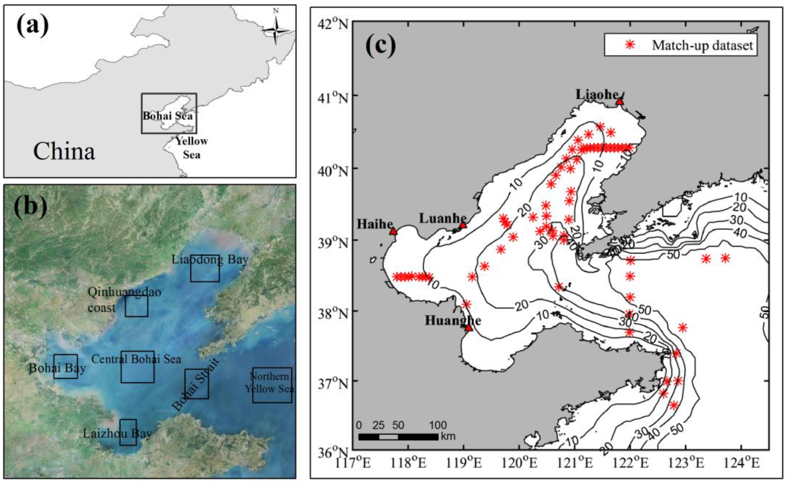
The Bohai Sea, located in northern China, is a shallow shelf sea with an average water depth of 18 m (with maximum depth of 80 m) and a total area of 77,000 km2 [30] (Figure 1). It is connected to the Yellow Sea through the Bohai Strait. Numerous inland rivers flow into the Bohai Sea from Mainland China with a total annual runoff of 8.88 × 10¹⁰ m3, nearly half of which comes from the Huanghe (Yellow River) [31]. The Bohai Sea is important as the main fishing ground and base of the marine fishery resources in northern China. Over the past several decades, the Bohai Sea has been influenced by human activity (e.g., agriculture, and industrial and domestic sewage) [32]. The Bohai Sea ecosystem has been gradually deteriorating due to red-tide events and eutrophication [33,34].
In this study, the Bohai Sea was subdivided into six sub-regions, following geographical regions (Figure 1b), including Liaodong bay (156 pixels), Qinhuangdao coast (144 pixels), Bohai bay (169 pixels), Laizhou bay (128 pixels), central Bohai Sea (256 pixels), and Bohai strait (165 pixels). The areas along the coastline of the Bohai Sea were excluded because of high levels of suspended sediment, which may increase the uncertainties of satellite-derived Chl-a [35,36]. Meanwhile, the northern Yellow Sea (400 pixels) was distinguished separately as a specific region. All clusters of pixels were isolated as regions of interest, and the data were averaged within each sub-region.
2.2. In Situ Chl-a Data
The in situ Chl-a data used in this study were collected during three cruises in June 2005, July 2011, and September 2012 in the Bohai Sea. Additionally, the Chl-a data collected during August 2015, June 2016, and December 2016 in the Bohai and northern Yellow Seas were also used in the algorithm validation, although the collecting time of these data was beyond that of our study period, because using the more data may give more reliable validation result. In total, the in situ dataset included 367 Chl-a samples.
For Chl-a analysis, seawater samples at the near surface (0–3 m) were collected using 12-liter Niskin bottles mounted on a CTD system. Water samples were filtered through 25-mm Whatman GF/F glass fiber filters under low vacuum pressure (<0.01 Mpa). After filtration, these samples were stored in liquid nitrogen until analysis in the laboratory. Prior to analysis, chlorophyllous pigments were extracted with N,N-dimethylformamide (DMF) for 24 h at 0 °C in the dark. Then, the florescence values of each sample, in fluorescent standard units (FSU), were measured three times using a Turner Design Fluorometer Model, and averaged these three measurements. Finally, the Chl-a was calculated from the corresponding florescence values based on the calibration curves.
2.3. Satellite Data
The daily remote sensing reflectance Rrs products of MODIS and SeaWiFS were acquired from the NASA ocean color website (http://oceancolour.gsfc.nasa.gov/). This dataset spanned 2000 to 2012 for a rectangular region (36–42°N and 117–124°E) that encompassed our study region. Additionally, the Level 3 monthly SST and PAR data with global coverage during our study period were obtained from the NASA ocean color website. These products were all cropped to the Bohai Sea. In addition, the bathymetric data were obtained from the ETOPO5 data (Earth Topography-5 Minute) at https://www.ngdc.noaa.gov/mgg/global/etopo5.html.
2.4. Chl-a Algorithm
In this study, we used the Chl-a algorithm of Siswanto et al. [24] to obtain satellite-derived Chl-a data. In regions with nLw555 > 2 mW·cm−2·μm−1·sr−1, the regionally tuned Tassan-like algorithm was used:
Under the low range of nLw555 (<2 mW·cm−2·μm−1·sr−1), the regionally tuned OC4v4 algorithm was used:
where R is a function of spectra value and Rrs(λ) is the remote sensing reflectance value at a given wavelength. Note that the invalid Rrs pixels were masked out based on the level 2 flagged pixels of the standard Rrs product. The daily Chl-a data were composed into monthly averages to match the SST and PAR datasets.
To assess the performance of the Chl-a retrieval algorithm, the coefficient of determination (R2), root mean square error (RMSE), and mean absolute percentage error (MAPE) were calculated between satellite-derived Chl-a and these measured values as below:
where n is the number of samples, and xi,derived and xi,field denote satellite-derived and in situ Chl-a data for the i-th sample, respectively.
2.5. Calculation of Trend and Information Flow
The linear trend model is commonly used in environmental and climate change research. The trend was obtained by: (1) subtracting the monthly climatological mean values from each corresponding month to remove the seasonal signal (producing monthly anomaly) [37]; and (2) calculating the linear trend using linear regression analysis. The line trend was the slope of the linear regression line for the time series of monthly anomaly, and its statistical significance was assessed with a statistical F-test. It is worth emphasizing that the linear trend in this study was assessed under a high percentage (>70%) of valid pixels to the total number of the monthly anomaly. If the percentage of valid pixels is too small (e.g., <30%), the trend statistical analysis may have large uncertainty due to insufficient valid data.
The correlation between different parameters is often detected using Pearson correlation analysis, but it is not designed to explore statistical dependencies between parameters [38]. In this study, we used a mathematical method based on the information flow (IF), which can quantitatively evaluate the cause and effect relation between time series [39]. The method was expressed as:
where T2→1 is the rate of information flowing from X2 to X1, Cij is the sample covariance between Xi and Xj, and Ci,dj is the covariance between Xi and dj. If the |T2→1| value is nonzero, there is causality between X2 and X1; if not, there is no causality between them. In this study, the Chl-a anomaly and SST (PAR) anomaly were symbolized by the subscripts “1”and “2” in Equation (7), respectively. The method could analyze the cause-effect relation and compare degrees of influence between different factors. It has been successfully applied to explain scientific problems in the real world. For instance, Liang [39] investigated the causal relation between the El Niño and Indian Ocean Dipole. Stips et al. [40] used this method to explore causality between different forcing components (e.g., anthropogenic, CO2, aerosol, cloud, and solar) and annual global mean surface temperature anomalies since 1850.
3. Results
3.1. Validation of Satellite-Derived Chl-a in the Bohai Sea
We applied the Chl-a algorithm of Siswanto et al. [24] to satellite data to investigate the Chl-a dynamics in the Bohai Sea. Before the application, the performance of the Chl-a algorithm was assessed based on 69 pairs of in situ Chl-a and satellite Rrs(λ) data (Figure 1c). This match-up dataset only consisted of satellite Rrs(λ) with an overpass time window within 5 h before and after field data. To avoid the effects of outliers, the median Rrs(λ) values for a 3 × 3 pixels window centered on the locations of the sampling stations were defined as satellite Rrs(λ). As shown in Figure 2, satellite-derived Chl-a generally agreed well with in situ Chl-a, with R2, RMSE and MAPE values of 0.53, 0.21 mg·m−3 and 38.38%, respectively. These results suggested that satellite-derived Chl-a in the Bohai Sea had high accuracy, which was considered generally acceptable in remote sensing research [24]. Therefore, we can further study the spatiotemporal variability of Chl-a in the Bohai Sea based on satellite-derived Chl-a.
3.2. Chl-a Spatial Distribution and Variability in the Bohai Sea
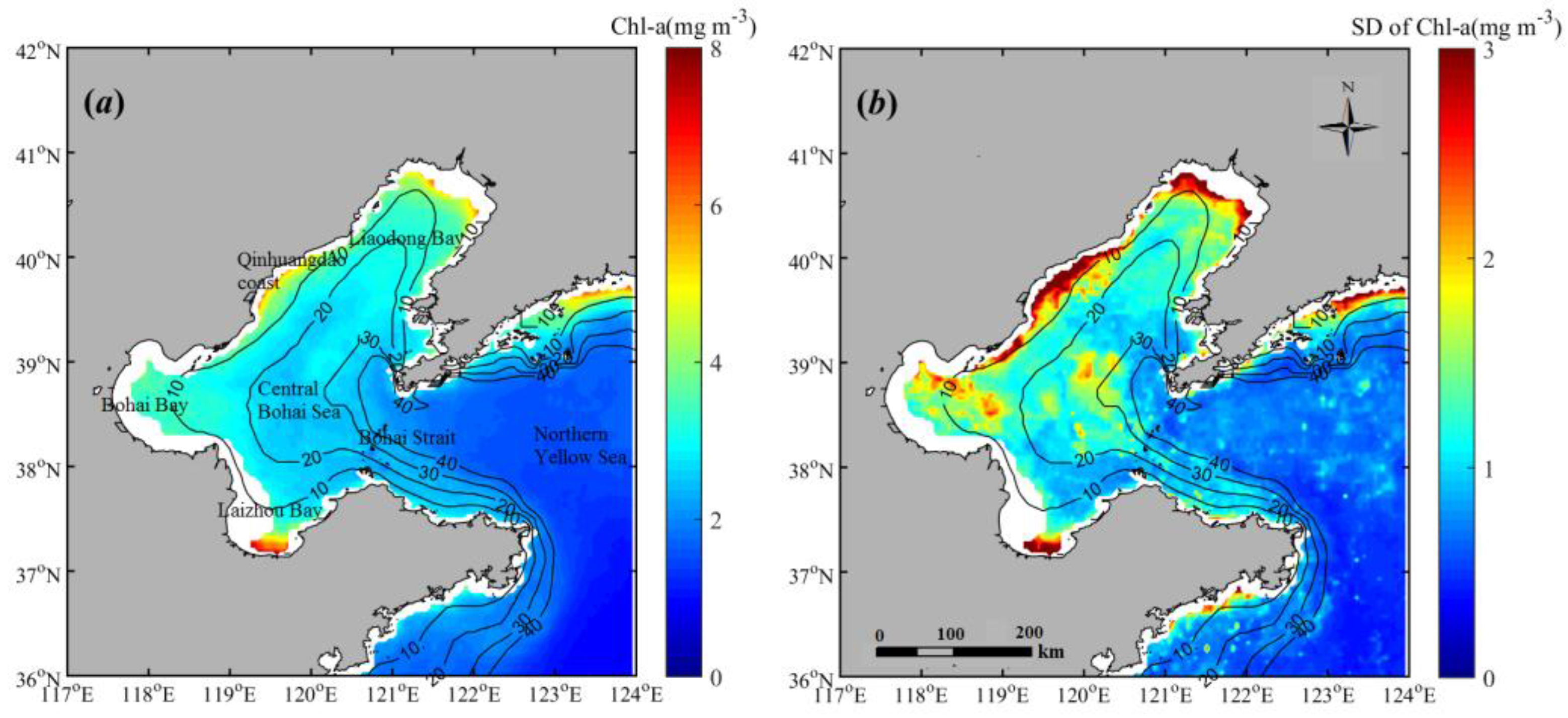
Using the monthly Chl-a data, the spatial and variability patterns of Chl-a were obtained by the temporal mean and standard deviation (SD) values during 2000–2012, respectively (Figure 3). In general, the Chl-a in the Bohai Sea showed much higher values than those in the northern Yellow Sea, and decreased gradually from coastal waters to offshore waters (Figure 3a). The highest Chl-a (>4.5 mg·m−3) were in the Qinhuangdao coast, southern Laizhou bay, and northern Liaodong bay. In addition, the relatively high Chl-a values (2.7–4.5 mg·m−3) were observed in coastal waters shallower than 20 m, whereas the relatively low values (<2.7 mg·m−3) were in the central Bohai Sea and Bohai strait. As shown in Figure 3b, the highest variability (SD > 2.5 mg·m−3) occurred in coastal area with <10 m isobaths. The higher variability (SD = 1.0–2.5 mg·m−3) were distributed in coastal waters and the central Bohai Sea, whereas lower variability (SD < 1 mg·m−3) appeared in the Bohai strait.
3.3. Chl-a Seasonal Patterns in the Bohai Sea
The seasonal patterns of Chl-a in each month from 2000 to 2012, represented by climatological monthly images, are shown in Figure 4. The seasonal dynamics of Chl-a in the Bohai Sea resulted in a growth process from May to September and depletion from October to April. The Chl-a values during winter and early spring (December–April) (with most of the values below 2.5 mg·m−3) were significantly lower than those from late spring to early autumn (May–September) (with most of the values above 3.5 mg·m−3). Figure 4e–j shows that the Chl-a was relatively higher (>6 mg·m−3) in coastal regions. The central Bohai Sea also had high Chl-a (>3 mg·m−3) from June to September (Figure 4f–i).
3.4. Area Difference in Seasonal Variations of Chl-a
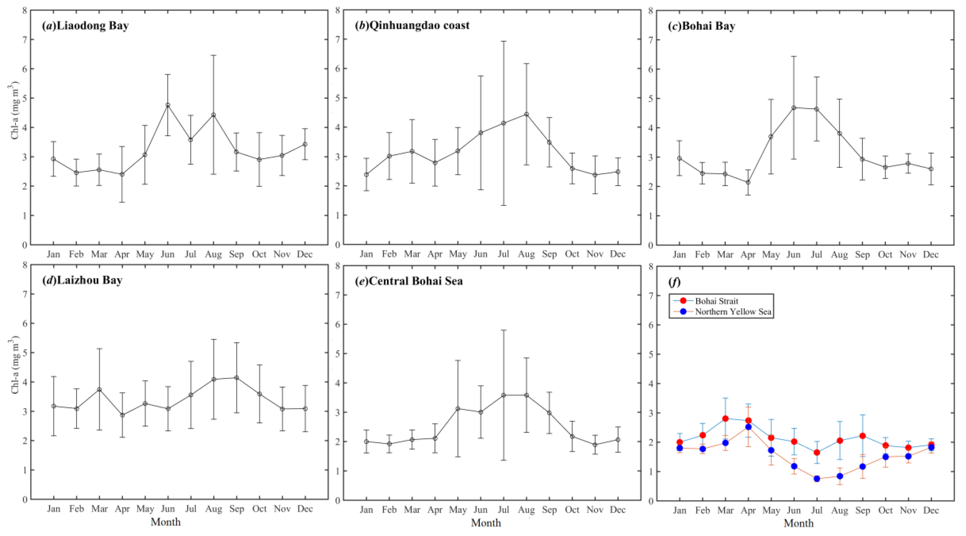
To gain more insight into seasonal variations of Chl-a over different locations, the Bohai Sea was divided into six sub-regions, as described in Section 2.1. The sampling area-averaged 13-year average of monthly Chl-a in the Bohai and northern Yellow Seas are shown in Figure 5. In the Liaodong bay, Qinhuangdao coast and Bohai bay, the seasonal patterns of Chl-a were characterized by a long-lasting Chl-a peak (>2.5 mg·m−3) from May to September (Figure 5a–c). However, in these three areas, seasonal maxima of Chl-a appeared in June (4.7 ± 1.0 mg·m−3), August (4.4 ± 1.7 mg·m−3), and June (4.7 ± 1.7 mg·m−3), respectively. In the central Bohai Sea (Figure 5d), the high Chl-a (>3 mg·m−3) was observed from May, decreased from September, and then remained relatively low during winter. The maximum Chl-a dominated in July or August (3.5 ± 2.0 mg·m−3). Two Chl-a maxima occurred in March (3.7 ± 1.4 mg·m−3) and September (4.1 ± 1.2 mg·m−3) in the Laizhou bay. However, the relatively low Chl-a was identified from April to June (Figure 5e), which was different from those in other coastal regions. Compared with other sub-regions, the Bohai strait had a distinct seasonal pattern of Chl-a with two Chl-a peaks in March (2.8 ± 0.7 mg·m−3) and September (2.2 ± 0.7 mg·m−3) and the lowest Chl-a in summer (Figure 5f). A similar seasonal pattern with the maximum in April (2.5 ± 0.6 mg·m−3) was identified in the northern Yellow Sea, but no maximum occurred in August or September.
3.5. Chl-a Trend in the Bohai Sea
The long-term trend of Chl-a in the Bohai Sea from 2000 to 2012 is shown in Figure 6. In general, the Chl-a trend values in the Bohai Sea were higher compared with those in the northern Yellow Sea. The upward trends (>0.0018 mg·m−3·month−1) were detected in the entire Bohai Sea, and its pattern was heterogeneous. The larger increase in Chl-a (>0.0035 mg·m−3·month−1) prevailed over coastal waters, especially in northern Liaodong bay and Qinhuangdao coast. The central Bohai Sea also had large positive trends (0.0025–0.0038 mg·m−3·month−1). It is noted that some coastal regions in the image, such as the Laizhou bay and Bohai bay, showed invalid pixels (white color) because of small percentage (<70%) of valid pixels.
In this study, spring, summer, autumn, and winter were defined as March to May, June to August, September to November, and December to February of the next year, respectively. The patterns of the Chl-a trend across four seasons are shown in Figure 7. Clear spatial and temporal variations of the Chl-a trend were observed in the Bohai Sea. In general, the Chl-a in the Bohai Sea displayed an increasing trend throughout the year. The Chl-a trend during summer and autumn showed higher values than those during winter and spring. At the temporal scale, the Chl-a trend was high in spring in the Bohai bay and Laizhou bay. In summer, the Chl-a trend was highest in most regions of the Bohai Sea, especially in the Bohai bay, Qinhuangdao coast, and central Bohai Sea. During autumn and winter, the Qinhuangdao coastal waters had high Chl-a trend.
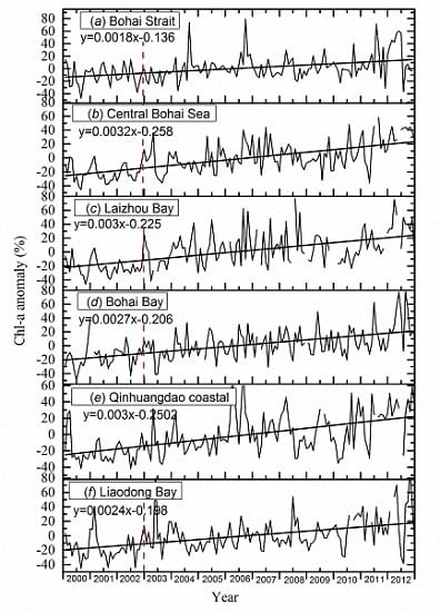
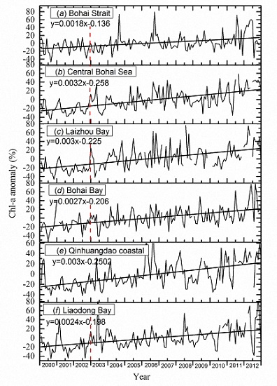
The inter-annual variations of Chl-a during 2000–2012 displayed different patterns for the six sub-regions of the Bohai Sea (Figure 8). All the sub-regions had an increasing trend: Bohai strait (0.0018), central Bohai Sea (0.0032), Laizhou bay (0.003), Bohai bay (0.0027), Qinhuangdao coast (0.003), and Liaodong bay (0.0024). The largest increase in Chl-a was observed in the central Bohai Sea, whereas the smallest increase in Chl-a was in the Bohai strait.
3.6. The Causality between Chl-a Anomaly, SST Anomaly, and PAR Anomaly
To assess the causality between Chl-a and SST and PAR in the Bohai Sea, we calculated the information flow from the SST anomaly to the Chl-a anomaly (hereafter referred to as IFSST→Chl-a) and those from the PAR anomaly to the Chl-a anomaly (hereafter referred to as IFPAR→Chl-a) in four seasons using Equation (7) (Figure 9). Clearly, both the IFSST→Chl-a and IFPAR→Chl-a values were nonzero in the areas marked by red (Figure 9a,b), in the sense that phytoplankton growth could be affected by PAR and SST in spring. As shown in Figure 9c,d, the IFPAR-Chl-a values were higher than IFSST→Chl-a. The IFPAR→Chl-a values in the Bohai Sea were above zero in summer, which indicated that PAR may be one of the factors affecting the growth of phytoplankton. During autumn, SST mainly showed significant IF in offshore waters (Figure 9e,f). IFSST→Chl-a was close to zero in the Bohai Sea in winter (Figure 9g), thus essentially no causality could be identified here. The causality between PAR and Chl-a occurred in most regions of the Bohai Sea in winter (Figure 9h). These results, as shown in Figure 9, implied that the influences of environmental drivers (PAR and SST) on the Chl-a pattern were complex, which has been confirmed by previous studies [22,41,42]. At this stage, it should be stated that we investigated the causality between Chl-a and SST by mainly considering the indirect influences of SST on Chl-a. This is because the changes in SST may induce stratification or mixing of the water column, which further alter the light and nutrient conditions and thereby impact the phytoplankton growth.
4. Discussion
4.1. The Chl-a Seasonal Patterns in the Bohai Sea
Our results on the seasonal patterns of Chl-a in the Bohai Sea, as shown in Figure 4 and Figure 5, revealed that the Chl-a varied on both spatial and temporal scales. To better understand these results, we focus on the discussion of the related physical and chemical effects and human activity on seasonal scale, combined with the causality between Chl-a and environmental factors (SST and PAR), as below.
In spring, the information flow shown in Figure 8a,b indicated that SST and PAR can affect phytoplankton growth [43]. Increased SST and solar radiation gradually reduce the vertical mixing of the water column. In addition, weak wind stress can retain vertical mixing, which enhances the transportation of the nutrient-rich bottom water to the euphotic layer [44]. This allows phytoplankton to live longer in the upper euphotic layer and acquire sufficient nutrients and more PAR for phytoplankton growth. Thus, the spring bloom occurred in our study regions, especially in the Qinhuangdao coast, Laizhou bay, Liaodong bay, and Bohai strait (Figure 5).
During summer, the causality between Chl-a and PAR was observed in the Bohai Sea (Figure 9d). Surface warming and low wind stress would increase the stratification of the water column. Theoretically, the stronger stratification and less mixing not only provide a higher percentage of PAR that is available for photosynthesis, but also lead to high water clarity and thereby deepen the euphotic layer depths. These conditions can favor phytoplankton growth. However, light may not be a limiting factor for controlling phytoplankton growth during summer. In contrast, the nutrient supply is expected to be an important factor in different regions [42].
Therefore, the nutrient conditions in different sub-regions of the Bohai Sea are discussed below to help understand the area differences in seasonal variations of Chl-a during summer. In the Bohai strait, the surface layer of the water column is stratified, preventing nutrient-rich waters from the deeper layer entering the photic zone. Meanwhile, all nutrients are depleted. Thus, the growth of phytoplankton is restricted, and the Chl-a reaches a minimum in summer (Figure 5). In contrast to the pattern in the Bohai strait, a pronounced Chl-a peak from May to September was observed in coastal water bodies (Liaodong bay, Qinhuangdao coast, and Bohai bay) and the central Bohai Sea. It may be related to the nutrients added by river discharge. Because of freshwater discharge from inland rivers carrying abundant nutrients, the trophic level in coastal waters increases significantly, especially in summer [45,46]. This has also been confirmed by Tang et al. [47] who reported that most harmful algal blooms may be initiated by nutrients from river discharge. Thus, the increased nutrients may support higher Chl-a levels in coastal waters. A question is why the central Bohai Sea also had higher Chl-a in summer. This may be attributed to water exchange between coastal waters and offshore waters related to the Bohai Sea circulation (including the warm current extension, Liaodong coastal current, and southern Bohai coastal current) and wind-tide-thermohaline circulation [19,48,49]. The water-exchange can enhance coastal nutrient transporting to the central Bohai Sea, thereby promoting the phytoplankton growth. Therefore, during summer, the nutrient supply from river discharge might be a major controlling factor in the high Chl-a in coastal waters and the central Bohai Sea. In contrast, the seasonal pattern of Chl-a in the Laizhou bay showed the relatively low Chl-a in early summer (Figure 5). Liu et al. [18] also reported this phenomenon in the sea region near the Yellow River mouth. This could be related to the water storage of dams and reservoirs on the Yellow River. The decreased riverine inputs due to dams and reservoirs can reduce the nutrient load, and thus result in the limitation for phytoplankton growth. Gong et al. [50] and Jiao et al. [51] reported that the decreased nutrient load and primary productivity during summer were associated with freshwater discharge reduction caused by water storages. In the Laizhou bay, human activity (e.g., dams and reservoirs) might be the reason for the change in Chl-a in early summer.
In autumn, the causality between SST and Chl-a (Figure 9e) indicated that the change in SST may influence the phytoplankton growth. With a decreasing SST and stronger wind stress, the stratification is broken down, and the vertical mixing of the water column increases, which could provide the nutrient supply and a suitable environment for phytoplankton growth. In the Bohai Sea, seasonal water stratification appears in April and breaks down at the end of September [47]. Thus, the relatively high Chl-a was observed in the Bohai Sea, such as the Bohai strait, Laizhou bay, central Bohai Sea, and Qinhuangdao coast (Figure 5).
When winter comes, stratification disappears and vertical mixing of the water column becomes strong due to sea surface cooling and strong winds. A strong northerly monsoon wind from late November to March influences the Bohai Sea [52], which can increase the mixing in the water column. Nutrients are carried to the surface layer from underlying nutrient-rich waters, which could provide for the spring bloom in the next year [53]. However, the low temperature and instability of the water column make it difficult to support an optimal growth condition for phytoplankton. In addition, mixing of the water column may decrease water transparency and increase the extinction coefficient of the upper water, which could reduce the amount of light available to phytoplankton. These offer an explanation to help us understand the relatively low Chl-a in winter (Figure 5). Due to the lack of field nutrient data, currently, we can only give a general discussion on the influence of nutrients on Chl-a. Further investigations focusing on this topic are still required in the future, when nutrient data become available.
4.2. The Increasing Trend of Chl-a in the Bohai Sea
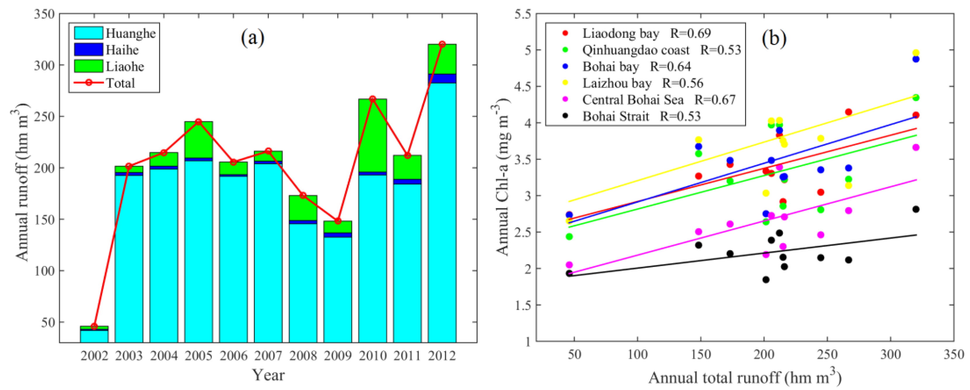
The entire Bohai Sea exhibited an increasing trend of Chl-a from 2000 to 2012 (Figure 5 and Figure 8). In particular, there were clear long-term increases in Chl-a since 2003 in the Laizhou bay, Bohai bay, Liaodong bay, Qinhuangdao coast, and central Bohai Sea (Figure 7b–f). There was a corresponding significant increase in the annual total runoff data of the three major rivers (Yellow River, Haihe River, and Liaohe River) since 2003, as shown in Figure 10a (date from Zhang et al. [54]). To further examine the relationship between the long-term changes in Chl-a and river runoff, we generated scatter plots to compare the annual Chl-a and annual total runoff for the six sub-regions of the Bohai Sea (Figure 10b). Although it is difficult to assess the effects of river discharge on the Chl-a trend in different sub-regions based only on 11-year time series data, we believe it is still useful to discuss their relationships. For these six sub-regions, the correlations between the annual Chl-a and annual total runoff were all positive, with high correlation coefficients (R ≥ 0.53), indicating that the increasing trend of Chl-a in the Bohai Sea might be influenced by river discharge. The freshwater discharge from riverine inputs supplies large amounts of nutrients to the Bohai Sea, favoring the phytoplankton growth. Furthermore, the nutrients added by inland rivers has increased significantly over the past several decades, mainly due to the use of chemical fertilizers and industrial/domestic sewage discharge [55]. Similarly, Li et al. [56] reported that eutrophication in the Qinhuangdao coast was mainly affected by nutrients from river discharge. Additionally, the higher and the lowest correlation coefficients were in the central Bohai Sea and Bohai strait, respectively. This might offer an explanation for the different increases in Chl-a in the central Bohai Sea and Bohai strait (Figure 7). The coastal nutrient can be transposed to offshore waters by currents and wind-tide-thermohaline circulation [47,57]. Meanwhile, because of the limitation of the Bohai strait, the central Bohai Sea has a longer water exchange with the Yellow Sea, and thus, the long retention time can increase nutrient concentrations, which further promotes an increase in Chl-a [58]. In contrast, the high water-exchange ability in the Bohai strait leads to nutrients in a shorter retention time and limits the increase trend of Chl-a. However, it is noted that we only showed the relationship between the Chl-a and riverine inputs over a relatively short timescale (11 years). Longer time series data with high temporal resolution (e.g., monthly) are needed to reveal the influence of river discharge on the Chl-a trends in the future when more data become available.
5. Conclusions
This study investigated the Chl-a dynamics in the Bohai Sea using satellite-derived products. The seasonal patterns of Chl-a displayed a long-lasting summer peak (May–September) in the Liaodong bay, Qinhuangdao coast, Bohai bay, and the central Bohai Sea. The relatively low Chl-a in early summer occurred in the Laizhou bay. In the Bohai strait, the two seasonal peaks appeared in March and September, and the minimum Chl-a was observed in summer. These variations of Chl-a could be mainly explained by the vertical structure of the water column, climate conditions (e.g., SST), and human activity. Meanwhile, the inter-annual patterns of Chl-a from 2000 to 2012 showed an increasing trend in the entire Bohai Sea, particularly in the central Bohai Sea, which might be related to river discharge. To better understand the long-term changes in Chl-a and its mechanisms, further efforts should be dedicated to making more detailed materials available (e.g., nutrient, water quality, and wind).
Acknowledgments
This research was jointly supported by the National Natural Science Foundation of China (Nos. 41576172, 41506200, and 41276186), the National Key Research and Development Program of China (No. 2016YFC1400901), the Provincial Natural Science Foundation of Jiangsu in China (Nos. BK20151526, BK20150914, and BK20161532), the National Program on Global Change and Air-sea Interaction (No. GASI-03-03-01-01), the Public Science and Technology Research Funds Projects of Ocean (201005030), a project funded by “the Priority Academic Program Development of Jiangsu Higher Education Institutions (PAPD)”, and the Research and Innovation Project for College Graduates of Jiangsu Province (1344051601032). Special thanks to Shaojie Sun in University of South Florida for data support.
Author Contributions
Hailong Zhang designed this study; Zhongfeng Qiu contributed to the data analyses and drafted the manuscript; Deyong Sun and Shengqiang Wang assisted with developing the research design and results interpretation; and Yijun He contributed to the interpretation of result.
Conflicts of Interest
The authors declare no conflict of interest.
References
- Field, C.B.; Behrenfeld, M.J.; Randerson, J.T.; Falkowski, P. Primary Production of the Biosphere: Integrating Terrestrial and Oceanic Components. Science. 1998, 281, 237–240. [Google Scholar] [CrossRef] [PubMed]
- Boyce, D.G.; Lewis, M.R.; Worm, B. Global phytoplankton decline over the past century. Nature. 2010, 466, 591–596. [Google Scholar] [CrossRef] [PubMed]
- Roemmich, D.; Mcgowan, J. Climatic Warming and the Decline of Zooplankton in the California Current. Science. 1995, 267, 1324–1326. [Google Scholar] [CrossRef] [PubMed]
- Chassot, E.; Bonhommeau, S.; Dulvy, N.K.; Watson, R.; Gascuel, D.; Pape, O.L. Global marine primary production constrains fisheries catches. Ecol. Lett. 2010, 13, 495–505. [Google Scholar] [CrossRef] [PubMed]
- Henson, S.A.; Sarmiento, J.L.; Dunne, J.P.; Bopp, L.; Lima, I.; Doney, S.C.; John, J.; Beaulieu, C. Detection of anthropogenic climate change in satellite records of ocean chlorophyll and productivity. Biogeosciences. 2010, 7, 621–640. [Google Scholar] [CrossRef]
- Sun, D.; Hu, C.; Qiu, Z.; Cannizzaro, J.P.; Barnes, B.B. Influence of a red band-based water classification approach on chlorophyll algorithms for optically complex estuaries. Remote Sens. Environ. 2014, 155, 289–302. [Google Scholar] [CrossRef]
- Maritorena, S.; Siegel, D.A.; Peterson, A.R. Optimization of a semianalytical ocean color model for global-scale applications. Appl. Opt. 2002, 41, 2705–2714. [Google Scholar] [CrossRef] [PubMed]
- Tassan, S. Local algorithms using SeaWiFS data for the retrieval of phytoplankton, pigments, suspended sediment, and yellow substance in coastal waters. Appl. Opt. 1994, 33, 2369–2378. [Google Scholar] [CrossRef] [PubMed]
- Tang, J.; Wang, X.; Song, Q.; Li, T.; Chen, J.; Huang, H.; Ren, J. The statistic inversion algorithms of water constituents for the Huanghai Sea and the East China Sea. Acta Oceanol. Sin. 2004, 23, 617–626. [Google Scholar]
- O’Reilly, J.E.; Maritorena, S.; Mitchell, B.G.; Siegel, D.A.; Carder, K.L.; Garver, S.A.; Kahru, M.; Mcclain, C. Ocean color chlorophyll algorithms for SeaWiFS. J. Geophys. Res. Oceans 1998, 103, 24937–24950. [Google Scholar] [CrossRef]
- Harley, C.D.G.; Hughes, A.R.; Hultgren, K.M.; Miner, B.G.; Sorte, C.J.B.; Thornber, C.S.; Rodriguez, L.F.; Tomanek, L.; Williams, S.L. The impacts of climate change in coastal marine systems. Ecol. Lett. 2006, 9, 228–241. [Google Scholar] [CrossRef] [PubMed]
- Smetacek, V.; Cloern, J.E. On Phytoplankton Trends. Science. 2008, 319, 1346–1348. [Google Scholar] [CrossRef] [PubMed]
- Tan, J.; Cherkauer, K.A.; Chaubey, I.; Troy, C.D.; Essig, R. Water quality estimation of River plumes in Southern Lake Michigan using Hyperion. J. Gt. Lakes Res. 2016, 42, 524–535. [Google Scholar] [CrossRef]
- Gong, G.-C.; Wen, Y.-H.; Wang, B.-W.; Liu, G.-J. Seasonal variation of chlorophyll a concentration, primary production and environmental conditions in the subtropical East China Sea. Deep Sea Res. Part II Top. Stud. Oceanogr. 2003, 50, 1219–1236. [Google Scholar] [CrossRef]
- Shi, W.; Wang, M. Satellite views of the Bohai Sea, Yellow Sea, and East China Sea. Prog. Oceanogr. 2012, 104, 30–45. [Google Scholar] [CrossRef]
- Yamaguchi, H.; Kim, H.C.; Son, Y.B.; Sang, W.K.; Okamura, K.; Kiyomoto, Y.; Ishizaka, J. Seasonal and summer interannual variations of SeaWiFS chlorophyll a in the Yellow Sea and East China Sea. Prog. Oceanogr. 2012, 105, 22–29. [Google Scholar] [CrossRef]
- He, X.Q.; Bai, Y.; Pan, D.L.; Chen, C.-T.A.; Cheng, Q.; Wang, D.F.; Gong, F. Satellite views of seasonal and inter-annual variability of phytoplankton blooms in the eastern China seas over the past 14 years (1998–2011). Biogeosci. Discuss. 2013, 10, 111–155. [Google Scholar] [CrossRef]
- Liu, D.; Wang, Y. Trends of satellite derived chlorophyll-a (1997–2011) in the Bohai and Yellow Seas, China: Effects of bathymetry on seasonal and inter-annual patterns. Prog. Oceanogr. 2013, 116, 154–166. [Google Scholar] [CrossRef]
- Guan, B.X. Patterns and Structures of the Currents in Bohai, Huanghai and East China Seas. In Oceanology of China Seas; Springer: Dordrecht, The Netherlands, 1994. [Google Scholar]
- Zhao, B.; Zhuang, G.; Cao, D.; Lei, F. Circulation, tidal residual currents and their effects on the sedimentations in the Bohai Sea. Oceanol. Limnol. Sin. 1995, 26, 466–473. [Google Scholar]
- Zhang, Y.; He, X.; Gao, Y. Preliminary analysis on the modified water massea in the north Yellow Sea and the Bohai Sea. Trans. Oceanol. Limnol. 1983, 2, 19–26. (In Chinese) [Google Scholar]
- Jackson, J.M.; Thomson, R.E.; Brown, L.N.; Willis, P.G.; Borstad, G.A. Satellite chlorophyll off the British Columbia Coast, 1997–2010. J. Geophys. Res. Oceans. 2015, 120, 4709–4728. [Google Scholar] [CrossRef]
- Jamet, C.; Loisel, H.; Kuchinke, C.P.; Ruddick, K.; Zibordi, G.; Feng, H. Comparison of three SeaWiFS atmospheric correction algorithms for turbid waters using AERONET-OC measurements. Remote Sens. Environ. 2011, 115, 1955–1965. [Google Scholar] [CrossRef]
- Siswanto, E.; Tang, J.; Yamaguchi, H.; Ahn, Y.H.; Ishizaka, J.; Yoo, S.; Kim, S.W.; Kiyomoto, Y.; Yamada, K.; Chiang, C. Empirical ocean-color algorithms to retrieve chlorophyll-a, total suspended matter, and colored dissolved organic matter absorption coefficient in the Yellow and East China Seas. J. Oceanogr. 2011, 67, 627–650. [Google Scholar] [CrossRef]
- Yamaguchi, H.; Ishizaka, J.; Siswanto, E.; Son, Y.B.; Yoo, S.; Kiyomoto, Y. Seasonal and spring interannual variations in satellite-observed chlorophyll-a in the Yellow and East China Seas: New datasets with reduced interference from high concentration of resuspended sediment. Cont. Shelf Res. 2013, 59, 1–9. [Google Scholar] [CrossRef]
- Terauchi, G.; Tsujimoto, R.; Ishizaka, J.; Nakata, H. Preliminary assessment of eutrophication by remotely sensed chlorophyll-a in Toyama Bay, the Sea of Japan. J. Oceanogr. 2014, 70, 175–184. [Google Scholar] [CrossRef]
- Ryu, J.H.; Han, H.J.; Cho, S.; Park, Y.J.; Ahn, Y.H. Overview of geostationary ocean color imager (GOCI) and GOCI data processing system (GDPS). Ocean Sci. J. 2012, 47, 223–233. [Google Scholar] [CrossRef]
- Qiu, Z.; Zheng, L.; Zhou, Y.; Sun, D.; Wang, S.; Wu, W. Innovative GOCI algorithm to derive turbidity in highly turbid waters: A case study in the Zhejiang coastal area. Opt. Express. 2015, 23, A1179–A1193. [Google Scholar] [CrossRef] [PubMed]
- Yuan, Y.; Qiu, Z.; Sun, D.; Wang, S.; Yue, X. Daytime sea fog retrieval based on GOCI data: A case study over the Yellow Sea. Opt. Express. 2016, 24, 787–801. [Google Scholar] [CrossRef] [PubMed]
- Qiu, Z. A simple optical model to estimate suspended particulate matter in Yellow River Estuary. Opt. Express 2013, 21, 27891–27904. [Google Scholar] [CrossRef] [PubMed]
- Zhou, H.; Zhang, Z.N.; Liu, X.S.; Tu, L.H.; Yu, Z.S. Changes in the shelf macrobenthic community over large temporal and spatial scales in the Bohai Sea, China. J. Mar. Syst. 2007, 67, 312–321. [Google Scholar] [CrossRef]
- Liu, S.M.; Zhang, J.; Chen, H.T.; Zhang, G.S. Factors influencing nutrient dynamics in the eutrophic Jiaozhou Bay, North China. Prog. Oceanogr. 2005, 66, 66–85. [Google Scholar] [CrossRef]
- Gao, X.; Zhou, F.; Chen, C.-T.A. Pollution status of the Bohai Sea: an overview of the environmental quality assessment related trace metals. Environ. Int. 2014, 62, 12–30. [Google Scholar] [CrossRef] [PubMed]
- Peng, S. The nutrient, total petroleum hydrocarbon and heavy metal contents in the seawater of Bohai Bay, China: Temporal–spatial variations, sources, pollution statuses, and ecological risks. Mar. Pollut. Bull. 2015, 95, 445–451. [Google Scholar] [CrossRef] [PubMed]
- Gong, G.-C. Absorption coefficients of colored dissolved organic matter in the surface waters of the East China Sea. Terr. Atmos. Ocean. Sci. 2004, 15, 75–88. [Google Scholar] [CrossRef]
- Cheng, C.; Huang, H.; Liu, C.; Jiang, W. Challenges to the representation of suspended sediment transfer using a depth-averaged flux. Earth Surf. Process. Landf. 2016, 41, 1337–1357. [Google Scholar] [CrossRef]
- Gregg, W.W.; Casey, N.W.; Mcclain, C.R. Recent trends in global ocean chlorophyll. Geophys. Res. Lett. 2005, 32, 259–280. [Google Scholar] [CrossRef]
- Sies, H. A new parameter for sex education. Nature 1988, 332. [Google Scholar] [CrossRef]
- Liang, X.S. Unraveling the cause-effect relation between time series. Phys. Rev. E. 2014, 90, 052150. [Google Scholar] [CrossRef] [PubMed]
- Stips, A.; Macias, D.; Coughlan, C.; Garcia-Gorriz, E.; San Liang, X. On the causal structure between CO2 and global temperature. Sci. Rep. 2016, 6, 21691. [Google Scholar] [CrossRef] [PubMed]
- Lin, C.; Su, J.; Xu, B.; Tang, Q. Long-term variation of temperature and salinity of the Bohai Sea and their influence on its ecosystem. Prog. Oceanogr. 2001, 49, 7–19. [Google Scholar] [CrossRef]
- Waite, J.N.; Mueter, F.J. Spatial and temporal variability of chlorophyll-a concentrations in the coastal Gulf of Alaska, 1998–2011, using cloud-free reconstructions of SeaWiFS and MODIS-Aqua data. Prog. Oceanogr. 2013, 116, 179–192. [Google Scholar] [CrossRef]
- Fennel, K. Convection and the timing of phytoplankton spring blooms in the western Baltic Sea. Estuar. Coast. Shelf Sci. 1999, 49, 113–128. [Google Scholar] [CrossRef]
- Behrenfeld, M.J.; O’Malley, R.T.; Siegel, D.A.; McClain, C.R.; Sarmiento, J.L.; Feldman, G.C.; Milligan, A.J.; Falkowski, P.G.; Letelier, R.M.; Boss, E.S. Climate-driven trends in contemporary ocean productivity. Nature 2006, 444, 752–755. [Google Scholar] [CrossRef] [PubMed]
- Lin, C.; Ning, X.; Su, J.; Lin, Y.; Xu, B. Environmental changes and the responses of the ecosystems of the Yellow Sea during 1976–2000. J. Mar. Syst. 2005, 55, 223–234. [Google Scholar] [CrossRef]
- Ye, L.; Yujie, Z.; Shitao, P.; Qixing, Z.; Ma, L.Q. Temporal and spatial trends of total petroleum hydrocarbons in the seawater of Bohai Bay, China from 1996 to 2005. Mar. Pollut. Bull. 2010, 60, 238–243. [Google Scholar]
- Tang, D.; Kawamura, H.; Oh, I.S.; Baker, J. Satellite evidence of harmful algal blooms and related oceanographic features in the Bohai Sea during autumn 1998. Adv. Space Res. 2006, 37, 681–689. [Google Scholar] [CrossRef]
- Sündermann, J.; Feng, S. Analysis and modelling of the Bohai sea ecosystem—A joint German-Chinese study. J. Mar. Syst. 2004, 44, 127–140. [Google Scholar] [CrossRef]
- Ning, X.; Lin, C.; Su, J.; Liu, C.; Hao, Q.; Le, F.; Tang, Q. Long-term environmental changes and the responses of the ecosystems in the Bohai Sea during 1960–1996. Deep Sea Res. Part II Top. Stud. Oceanogr. 2010, 57, 1079–1091. [Google Scholar] [CrossRef]
- Gong, G.-C.; Chang, J.; Chiang, K.-P.; Hsiung, T.-M.; Hung, C.-C.; Duan, S.-W.; Codispoti, L.A. Reduction of primary production and changing of nutrient ratio in the East China Sea: Effect of the Three Gorges Dam? Geophys. Res. Lett. 2006, 33. [Google Scholar] [CrossRef]
- Jiao, N.; Zhang, Y.; Zeng, Y.; Gardner, W.D.; Mishonov, A.V.; Richardson, M.J.; Hong, N.; Pan, D.; Yan, X.H.; Jo, Y.H. Ecological anomalies in the East China Sea: Impacts of the Three Gorges Dam? Water Res. 2007, 41, 1287–1293. [Google Scholar] [CrossRef] [PubMed]
- Yuan, Y.; Su, J. Numerical modeling of the circulation in the East China Sea. Ocean Hydrodyn. Jpn. East China Seas. 1984, 39, 167–176. [Google Scholar]
- Yamada, K.; Ishizaka, J.; Yoo, S.; Kim, H.C.; Chiba, S. Seasonal and interannual variability of sea surface chlorophyll a concentration in the Japan/East Sea (JES). Prog. Oceanogr. 2004, 61, 193–211. [Google Scholar] [CrossRef]
- Zhang, M.; Dong, Q.; Cui, T.; Ding, J. Remote Sensing of Spatiotemporal Variation of Apparent Optical Properties in Bohai Sea. IEEE J. Sel. Top. Appl. Earth Obs. Remote Sens. 2015, 8, 1176–1184. [Google Scholar] [CrossRef]
- Qu, H.J.; Kroeze, C. Past and future trends in nutrients export by rivers to the coastal waters of China. Sci. Total Environ. 2010, 408, 2075–2086. [Google Scholar] [CrossRef] [PubMed]
- Li, Z.; Cui, L. Contaminative conditions of main rivers flowing into the sea and their effect on seashore of Qinhuangdao. Ecol. Environ. Sci. 2012, 21, 1285–1288. (In Chinese) [Google Scholar]
- Hickox, R.; Belkin, I.; Cornillon, P.; Shan, Z. Climatology and seasonal variability of ocean fronts in the East China, Yellow and Bohai seas from satellite SST data. Geophys. Res. Lett. 2000, 27, 2945–2948. [Google Scholar] [CrossRef]
- Wei, H.; Sun, J.; Moll, A.; Zhao, L. Phytoplankton dynamics in the Bohai Sea—Observations and modelling. J. Mar. Syst. 2004, 44, 233–251. [Google Scholar] [CrossRef]
Figure 1.
Location of the Bohai Sea (a) and the sampling locations of sub-regions, which are marked by squares (b), namely, Liaodong bay, Qinhuangdao coast, Bohai bay, Laizhou bay, central Bohai Sea, Bohai strait, and northern Yellow Sea. Locations of the match-up stations in the Bohai and northern Yellow Seas (c).

Figure 2.
Comparison of satellite-derived Chl-a with in situ measured values.

Figure 3.
Distribution of the mean (a) and standard deviation (b) values of satellite-derived Chl-a during 2000–2012. The invalid pixels in the image are indicated by the white color.
Figure 3.
Distribution of the mean (a) and standard deviation (b) values of satellite-derived Chl-a during 2000–2012. The invalid pixels in the image are indicated by the white color.

Figure 4.
(a–l) Monthly climatological Chl-a images in the Bohai Sea during 2000–2012. The invalid pixels in the image are indicated by the white color.
Figure 4.
(a–l) Monthly climatological Chl-a images in the Bohai Sea during 2000–2012. The invalid pixels in the image are indicated by the white color.

Figure 5.
(a–f) Seasonal variation in 13-year averaged monthly Chl-a from January to December in seven sub-regions.
Figure 5.
(a–f) Seasonal variation in 13-year averaged monthly Chl-a from January to December in seven sub-regions.

Figure 6.
The long-term trend of monthly Chl-a anomaly from 2000 to 2012. The invalid pixels in the image are indicated by the white color.
Figure 6.
The long-term trend of monthly Chl-a anomaly from 2000 to 2012. The invalid pixels in the image are indicated by the white color.

Figure 7.
(a–d) The long-term trends of Chl-a anomaly in four seasons from 2000 to 2012.

Figure 8.
Linear trends of the Chl-a anomaly in the six sub-regions of the Bohai Sea. The black lines represent the linear trend, and the red lines represent the scratch line of the year 2003, as mentioned in Section 4.2.
Figure 8.
Linear trends of the Chl-a anomaly in the six sub-regions of the Bohai Sea. The black lines represent the linear trend, and the red lines represent the scratch line of the year 2003, as mentioned in Section 4.2.

Figure 9.
(a–h) The spatial distribution of information flow from the SST (PAR) anomaly to the Chl-a anomaly.
Figure 9.
(a–h) The spatial distribution of information flow from the SST (PAR) anomaly to the Chl-a anomaly.
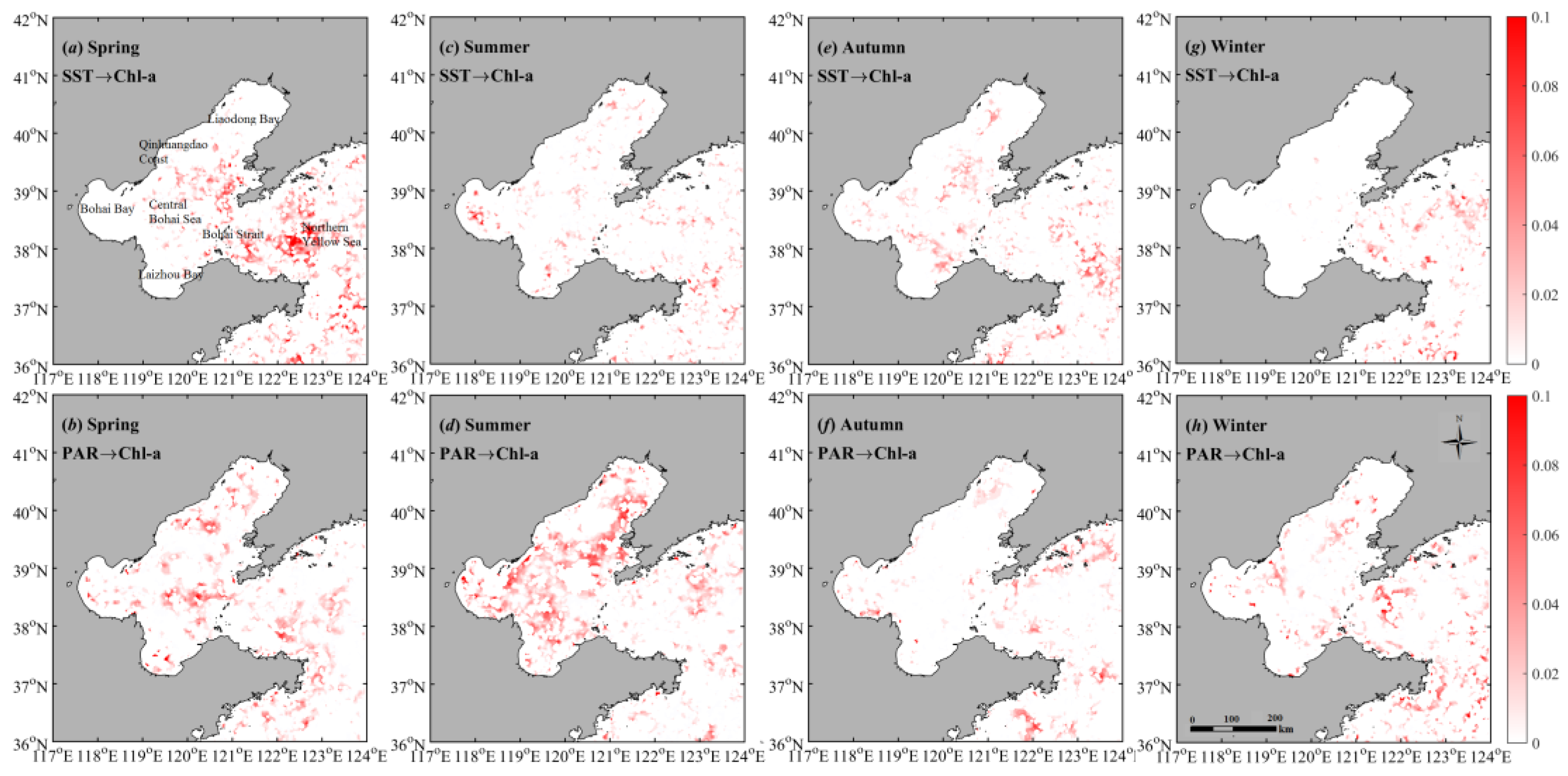
Figure 10.
The annual runoff data of the three major rivers from 2002 to 2011 (data from Zhang et al. [54]) (a). The scatter plots between the annual Chl-a of six sub-regions and the annual total runoff from 2002 to 2012 (b).
Figure 10.
The annual runoff data of the three major rivers from 2002 to 2011 (data from Zhang et al. [54]) (a). The scatter plots between the annual Chl-a of six sub-regions and the annual total runoff from 2002 to 2012 (b).

© 2017 by the authors. Licensee MDPI, Basel, Switzerland. This article is an open access article distributed under the terms and conditions of the Creative Commons Attribution (CC BY) license (http://creativecommons.org/licenses/by/4.0/).
Share and Cite
MDPI and ACS Style
Zhang, H.; Qiu, Z.; Sun, D.; Wang, S.; He, Y. Seasonal and Interannual Variability of Satellite-Derived Chlorophyll-a (2000–2012) in the Bohai Sea, China. Remote Sens. 2017, 9, 582. https://doi.org/10.3390/rs9060582
AMA Style
Zhang H, Qiu Z, Sun D, Wang S, He Y. Seasonal and Interannual Variability of Satellite-Derived Chlorophyll-a (2000–2012) in the Bohai Sea, China. Remote Sensing. 2017; 9(6):582. https://doi.org/10.3390/rs9060582
Chicago/Turabian StyleZhang, Hailong, Zhongfeng Qiu, Deyong Sun, Shengqiang Wang, and Yijun He. 2017. "Seasonal and Interannual Variability of Satellite-Derived Chlorophyll-a (2000–2012) in the Bohai Sea, China" Remote Sensing 9, no. 6: 582. https://doi.org/10.3390/rs9060582
Note that from the first issue of 2016, this journal uses article numbers instead of page numbers. See further details here.