Abstract
Edge detection is one of the key issues in the field of computer vision and remote sensing image analysis. Although many different edge-detection methods have been proposed for gray-scale, color, and multispectral images, they still face difficulties when extracting edge features from hyperspectral images (HSIs) that contain a large number of bands with very narrow gap in the spectral domain. Inspired by the clustering characteristic of the gravitational theory, a novel edge-detection algorithm for HSIs is presented in this paper. In the proposed method, we first construct a joint feature space by combining the spatial and spectral features. Each pixel of HSI is assumed to be a celestial object in the joint feature space, which exerts gravitational force to each of its neighboring pixel. Accordingly, each object travels in the joint feature space until it reaches a stable equilibrium. At the equilibrium, the image is smoothed and the edges are enhanced, where the edge pixels can be easily distinguished by calculating the gravitational potential energy. The proposed edge-detection method is tested on several benchmark HSIs and the obtained results were compared with those of four state-of-the-art approaches. The experimental results confirm the efficacy of the proposed method.
1. Introduction
With the development of optic-electronics and data transmission technologies, hyperspectral sensors are able to capture hundreds of spectral bands simultaneously with good spatial resolution. A few well-known hyperspectral imaging systems, such as AVIRIS (the Airborne Visible Infrared Imaging Spectrometer), HYDICE (the Hyperspectral Digital Imagery Collection Experiment), and EnMap (the Environmental Mapping and Analysis Program), can provide 126–512 spectral bands with a spatial resolution from 3 m to 30 m. The growing availability of hyperspectral images (HSIs) with both fine spectral and spatial resolution has opened the door to numerous new applications in remote sensing [1].
In many application areas for HSIs, segmentation is required as an important image processing step because it divides an image into meaningful homogeneous regions [2]. However, because the imaged scenes are complex scenes and may not have clear boundaries, image segmentation is always a big challenging task. Effective edge detection algorithms have been found useful for image segmentation since they delineate boundaries of regions and determine segmentation results [2,3]. Especially for the advanced HSIs with high spatial resolution, the clearly depicted edges could be of great benefit in characterizing the spatial structures of landscapes [4].
Over the past few decades, a large number of edge-detection techniques have been proposed, such as Canny [5], Marr [6], SUSAN (Univalue Segment Assimilating Nucleus) [7] and active contour based methods [8]. However, these approaches are designed primarily for gray, color or multispectral images and few studies have paid attention to edge detection on HSIs [9,10]. In previous studies [10,11], edge-detection tasks are completed by adapting color or multispectral approaches to hyperspectral images (HSIs). Accordingly, existing approaches for color or multispectral based edge detection are discussed as follows.
In general, most approaches for color or multispectral based edge detection can be grouped into three categories: (1) monochromatic approaches; (2) vector based approaches; and (3) feature-space based approaches. Monochromatic approaches combine all edge maps after applying well-established gray-scale edge detectors on each band, and typical rules for combining edges include the maximum rule [12], the summation rule [13] and the logic OR operation [14]. Although the fine spectral resolution of HSI provides invaluable and abundant information regarding the physical nature of different materials [10], edge features may be only observable over a small subset of bands in the HSI [15]. That is to say, different spectral bands may even contain inconsistent edges, which can easily leads to false edges by simple combination. To overcome this drawback caused by the combination rules, Lei and Fan combined the first principal component and hue component of color images to obtain complete object edges [16].
Different from monochromatic approaches, vector-based approaches consider each pixel as a spectral vector and then use vector operations to detect edges [17,18,19,20,21,22,23,24]. In these approaches, the gradient magnitude and direction are defined in a vector field by extending the gray-scale edge definition [11]. Di Zenzo’s gradient operator [17], which uses the tensor gradient to define the edge magnitude and direction, is a widely used vector-based method. However, Di Zeno’s method is sensitive to small changes in intensity because it is based on the measure of the squared local contrast variation of multispectral images. To overcome this problem, in Drewniok [19], Di Zeno’s method is combined with the Canny edge detector with a Gaussian pre-filter model applied to each band for smoothing the image. Drewniok’s method has better effectiveness, but it results in a localization error when the Gaussian scale parameter is large [25]. To remove both the effect of noise and the localization error caused by pre-filtering, a novel method based on robust color morphological gradient (RCMG) is proposed, where the edge strength of a pixel is defined as the maximum distance between any two pixels in its surrounding window [24]. The RCMG is robust to noise and helps top reserve accurate spatial structures due to a non-linear scheme is implied in the process [10].
Generally speaking, vector based approaches are superior to monochromatic approaches in multispectral edge detection since they take the spectral correlation of the bands into consideration. Different from color images or multispectral images, however, HSIs usually consist of hundreds of contiguous spectral bands. Although the high spectral resolution of HSIs provides potential for more accurate identification of targets, it still suffers from three problems in edge detection, various interferences that lead to low homogeneity inside regions [26], spectral mixtures or edges that appear in a small subset of bands often cause weak edges [26] and inconsistent edges from narrow and abundant channels [27], which have made edge detection more challenging in HSIs. Dimension reduction has been investigated using signal subspace approach and proposed the local rank based edge detection method [28], however the performance is limited. It is necessary to consider the spatial relationships between spectral vectors [29]. In Reference [30], a modified Simultaneous Spectral/Spatial Detection of Edges (SSSDE) [31] for HSIs was proposed to exploit spectral information and identify boundaries (edges) between different materials. This is a kind of constructive attempt to joint utilization of spatial and spectral information. Recently, many researchers have tried to develop feature-based new edge-detection methods because edge pixels have saliency in the feature space [32]. In Lin [32], color image edge detection is proposed based on a subspace classification in which multivariate features are utilized to determine edge pixels. In Dinh [27], MSI edge detection is achieved via clustering the gradient feature. The feature space is suitable to analyze HSIs because it is capable of showing data from various land cover types in groups [33]. In particular, a spatial-spectral joined feature space, which takes into consideration both the spatial and spectral correlation between pixels, has attracted increasing attention [1,29]. In addition to edge detection, feature space has also been widely used in other fields of image processing, such as hyperspectral feature selection [34,35], target detection [36], and image segmentation [37,38]. However, few studies focus on edge detection for HSIs using feature space.
Physical models that mimic real-world systems can be used to analyze complex scientific and engineering problems [37,39,40]. The ongoing research of physical models has motivated the exploration of new ways to handle image-processing tasks. As a typical physical model, Newton’s law of universal gravitation [41] has received considerable attention, based on which, a series of image-processing algorithms has been proposed, such as the stochastic gravitational approach to feature-based color image segmentation (SGISA) [37], the improved gravitational search algorithm for image multi-level image thresholding [42] and the gravitational collapse (CTCGC) approach for color texture classification [43]. Other gravitation model based approaches for classification include data gravitation classification (DGC) [44,45,46] and gravitational self-organizing maps (GSOM) [47]. The advantages of the gravity field model have inspired the development of new edge-detection method for gray-scale images [48,49]. Although the image-processing procedure using gravitational theory is relatively easy for understanding, this theory is rarely used in edge detection for HSIs. As the gravitational theory describes the movements of objects in the three-dimensional feature space of the real world, we can easily extend it to n-dimensional feature space and apply it for edge detection in HSIs.
In this paper, a novel edge-detection method for HSIs based on gravitation (GEDHSI) is proposed. The main ideas of the proposed GEDHSI are as follows: (1) there exists a type of “force”, called gravitation, between any two pixels in the feature space; (2) computational gravitation obeys the law of gravitation in the physical world; (3) all pixels move in the feature space according to the law of motion until the stopping criteria are satisfied, and then the image system reaches a stable equilibrium; and (4) the edge pixels and non-edge pixels are classified into two different clusters. Therefore, in the equilibrium system, edge responses can be obtained by computing the gravitational potential energy due to the relative positions. Different from our previous approach for gravitation based edge detection in gray-scale images [49], the proposed method features a dynamic scheme. By imitating the gravitational theory, all pixels move in the joint spatial-spectral feature space, which makes the GEDHSI more attractive and effective for HSIs. The experiment results illustrate both the efficiency and efficacy of the proposed method for HSI edge-detection problems.
The rest of the paper is organized as follows: The law of universal gravity is briefly reviewed in Section 2. The proposed gravitation-based edge detection method is presented in Section 3. The experimental validations of the proposed algorithm using both artificial and real HSIs are given in Section 4. Finally, the paper is concluded in Section 5.
2. Background of the Universal Law of Gravitation
According to gravitational theory [35], any two objects exert gravitational force onto each other. The forces between them are equal to each other but reverse in direction. The force is proportional to the product of the two masses and inversely proportional to the square of the distance between them, as shown in Equation (1):
where is the vector-form magnitude of the gravitational force between objects i and j, and their masses are denoted as and (), respectively. G is the universal gravitational constant, and represent the position vector of objects i and j. Newton’s second law says that when a force, , is applied to object i, its acceleration, , depends only on the force and its mass, [50]:
For , two types of mass are defined in theoretical physics:
Gravitational mass, , is a measure of the strength of the gravitational field due to a particular object. The gravitational field of an object with small gravitational mass is weaker than an object with larger gravitational mass.
Inertial mass, , is a measure of an object’s resistance to changing its state of motion when a force is applied. An object with large inertial mass changes its motion more slowly, and an object with small inertial mass changes it rapidly.
In physics, gravitational mass and inertial mass are usually treated as the same. In this paper, they are treated separately to enhance the adaptability of gravitational theory for HSI edge detection. That is to say, the gravitational force, , that acts on object i by object j is proportional to the product of the gravitational mass of objects j and i and inversely proportional to the square distance between them. is proportional to and inversely proportional to inertia mass of object i. More precisely, we rewrite Equations (1) and (2) as follows:
where and represent the gravitational mass of objects i and j, respectively. represents the inertial mass of object i.
The gravitational force obeys the superposition principle. Thus, for any object k in the space, the gravitational force exerted by objects i and j is calculated by Equation (5).
where is the position of object k in space , and is the gravitational mass of object k. The resultant force forms the gravitational field.
Because the gravitational field is conservative, there is a scalar potential energy (SPE) per unit mass at each point in the space associated within the gravitational fields. The SPE of object i exerted by object j is determined by Equation (6) [51] as follows:
Similar to the gravitational force, the SPE also obeys the superposition principle.
The SPE is closely linked with forces. It can be concluded that the force is the negative differential of the SPE [52], which is expressed as follows:
where is the delta operator. The SPE function is extendable to high dimensional feature space and capable of reflecting the inhomogeneity of data, which is a key point for edge detection.
In gravitational systems, all objects move under the gravitational force until an equilibrium phase is reached. In the equilibrium phase, all similar objects aggregate to form a cluster. Different clusters have different properties, such as SPE. Some gravitation-based algorithms are inspired from the characteristics of gravitational theory [37,50]. In this paper, we assume that edge and non-edge pixels are by nature two different clusters. Therefore, they will have different SPEs. These properties constitute the background of the proposed method.
3. Gravitation-Based Edge Detection in Hyperspectral Image (GEDHSI)
3.1. Overview
GEDHSI is proposed in this study based on the Newton’s law of universal gravitation. It contains three main phases as illustrated in Figure 1. The first phase is image mapping which maps a HSI into a joint spatial-spectral feature space, as detailed in Section 3.2. In the joint space, every pixel is considered as an object which attracts each other via the gravitational force. The second phase is the pixel traveling phase as detailed in Section 3.3 where an iterative procedure is used to allow all pixels move within the joint spatial-spectral feature space under the influence of the gravitational force until the image system reaches a stable equilibrium. In this state, the edge pixels and non-edge pixels will have different scalar potential energy (SPEs) based on their relative positions. Consequently, in the third phase, the edge response is obtained based on the determined SPE of each pixel.
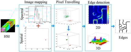
Figure 1.
Overview of the proposed GEDHSI (Gravitation-Based Edge Detection in Hyperspectral Image).
3.2. Image Mapping
The gravitational theory is derived from three-dimensional real-world space. To simulate the theory, we first need to map the HSI into a feature space. For a HSI denoted by , the parameters H, W and B represent height, the width of the image and the number of bands, respectively. A simple feature space is composed only of its bands. This type of feature space primarily uses spectral information. To make full use of spatial and spectral information, inspired by Reference [37], we define a spatial-spectral jointed feature space containing (B + 2) features (dimensions). In the feature space, each pixel addresses a location in the space:
where is the total number of pixels in the image, ) is the spectral components of the pixel i, and is its spatial position.
3.3. Pixel Traveling
Once the joint spatial-spectral feature space is constructed, we consider each pixel as a mass object in the space. Thereby, as introduced in Section 2, each pixel can attract others through the gravitational force and then moves in the joint feature space according to the gravitational theory. In other words, in the traveling stage, all objects move step by step within the joint feature space under the gravitational force until the stopping criteria are met. Specifically, the pixel traveling phase contains the following three steps in an iterative way until the whole image based system becomes stable:
- (1)
- Calculation of the acceleration;
- (2)
- Calculation of the traveling step size;
- (3)
- Location updating.
(1) Calculation of the Acceleration
In GEDHSI, for a pixel i at time t, its acceleration is computed according to Equation (9) as follow:
where is the gravitational force of the pixel i exerted by the other pixels at time t, and is the inertial mass of the pixel i at time t.
According to Equation (7), the gravitational force is proportional to the delta of SPE and along the decreased direction of SPE. Therefore, we first calculate the SPE of the pixels i produced by a pixel j as follows:
where is the distance between the pixels i and j, and and are the gravitational mass of the pixels i and j. In this paper, to simplify the calculation, gravitational mass of each object is set as a unit value.
Obviously, the distance is a dominant factor in Equation (10). The distance measure used in Equation (1) will result in singularity. To avoid this problem and make smooth and finite, the distance in GEDHSI is redefined by Equation (11), as follows:
where is the Euclidean distance between pixels i and j, and is an influence factor.
Then, by substituting Equations (10) and (11) into Equation (7), we can obtain the gravitational force of pixel i exerted by the pixel j as follows:
Because the gravitational force obeys the superposition principle, for a dataset D that consists of m pixels, the gravitational force of pixel i exerted by the dataset D is determined as the accumulated force for each pixel within D as follows:
According to Equation (13), the dataset D is a key factor for computing gravitational force. In general cases, all pixels are involved to compute the gravitational force. However, this will lead to high computational time. According to Equation (13), the gravitational force attenuates toward zero when the distance increases. Thus, for those pixels that exceed a pre-specified range, we can safely assume that their gravitational forces are zero to simplify the computation.
To this end, the dataset D can be constructed by
where r is the radius of a local circular window in the spatial domain, is the radius in the spectral domain, and j is the neighbor pixel around the pixel i. r and construct a local suprasphere in the feature space. Here, to balance the effect of the spatial and spectral distance, the position of each pixel is stretched in spectral domain by . Thus, the influence factor is equal to , and is replaced by . All pixels inside the suprasphere compose the dataset D.
According to Equation (9), in addition to resultant force, inertial mass is critical in the traveling procedure. In the proposed method, the inertial mass of pixel i, is defined as follows:
Obviously, the inertial mass is capable of capturing the local information with self-adaptation when traveling.
(2) Calculation of the Traveling Step
After obtaining the acceleration, we can calculate the traveling step size using the law of motion (Equation (16)).
where is the velocity of pixel i at time t. To make the pixel move directly toward the potential center, is considered zero in time. is the time interval in two adjacent iterations and is set to 1. Thus, Equation (16) is replaced by Equation (17):
(3) Location Updating
Based on the traveling step size, the location of the pixel i can be updated as follows:
The traveling procedure is an iterative procedure and will be repeated until the following stopping criteria are met: (1) the maximum step size where ; or (2) the iterations reach a maximum T. In this stage, each pixel moves along the direction of the associated gravitational force. By traveling, they can find other, similar pixels, which remove the influence of noise and preserves the structural detail.
3.4. Edge Detection
When the traveling stops, the image system reaches a stable equilibrium where similar pixels will cluster together. Thereby, due to the relative positions, different pixels have various SPEs. The SPE of each pixel can be calculated. For edge pixels, the SPE is relatively high, whereas for non-edge pixels, the SPE is relatively low. Thus, we take the SPE of each pixel as the edge response. The calculation of the SPE of each object is also restricted to the dataset D and using Equation (19).
Apparently, finding an appropriate threshold will classify the edge and non-edge pixels into two categories and the edge will be finally detected.
According to Reference [35], a good edge detection method should keep a thin and accurate localization of edges. To satisfy such requirements, information about edges’ directions is necessary for non-maximum suppression. In accordance with Reference [49], we first project the SPE to the horizontal and vertical directions in the spatial domain, as shown in Equation (20).
where and are the SPE of pixel i projected onto the horizontal and vertical directions, respectively. Then, the edge direction is estimated by Equation (21) as follows:
With and , non-maximum suppression and automatic hysteresis thresholding [53] can be applied to obtain the exact edge. Figure 2 depicts the flowchart of the proposed GEDHSI.
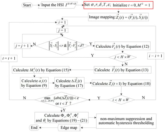
Figure 2.
Flowchart of the proposed GEDHSI.
4. Experimental Results and Discussion
To demonstrate the efficacy and efficiency of the proposed method, we carried out three groups of experimental validation, including quantitative and qualitative evaluation and CPU runtime. Group 1, was designed to quantitatively compare the performances of different edge detectors by using two artificial images, AI 1 and AI 2 (Section 4.3). Group 2 was designed to validate the performance of the proposed approach on two real remote sensing HSIs and two ground scene HSIs (Section 4.4). Group 3 was designed to test the computational efficiency of different edge detectors using the two remote sensing HSIs (Section 4.5). Detailed introduction of the tested data sets used in experiments and evaluation methods are given in Section 4.1 and Section 4.2, respectively.
In all experiments, all edge results were compared between the proposed method and four other state-of-the-art multispectral edge detection methods, which include those from Di Zenzo [17], Drewniok [19], RCMG [24] and SSSDE [30]. Di Zenzo initially used the Sobel operator as channel-wise gradient technique [17], which is sensitive to noise. To improve the anti-noise anility, we prefer to use the ANDD-based gradient [46,54] considering its superiority in noise robustness. It is worth noting that the implementation codes of the comparative methods are directly taken from the authors for fair and consistent comparison. We selected their optimized parameters by trial-error methods. The parameters of GEDHSI were set as , , and in this paper. The parameter was set to the same value as as discussed in Section 3.3. All the experiments were conducted under the following settings: Matlab2013a, 64 bit Windows 7 system, 2.9 GHz Intel Pentium CPU with 6 GB RAM.
4.1. Test Datasets
Six hyperspectral data sets in three groups that include two artificial ones and four real natural scenes are used in our experiments for performance assessment as listed in Table 1. The first two artificial images are synthesized using the HYDRA [55] which were used to evaluate the performance in dealing with background clutter and weak edges. The real HSIs include two remote sensing HSIs and two ground scene HSIs. The first remote sensing HSI is Farmland image is an AVIRIS flight line over a farmland of east-central Indiana [56]. Another remote sensing HSI is a HYDICE flight line over the Washington DC Mall [57]. The two ground scene HSIs are chosen from the Foster’s HSI dataset [58] to further investigate the performance of the proposed method on real ground scenes. All these images are suitable to evaluate the performance of connectivity, edge resolution and the ability to suppress false edges.

Table 1.
Properties of the data sets used in experiments.
4.2. Evaluation Methods
Most edge detection techniques utilize thinning and binarization to obtain the final edge results [59]. In this study, we put all these edge strength maps into the same thinning process. In this process, a pixel is only considered as an edge if it is a local maximum in the horizontal or vertical direction. Then, we applied the automatic threshold selection and hysteresis thresholding technique [53] on the edge strength maps to generate the binary edges.
We investigated edge detection results with both subjective and quantitative evaluations. For quantitative evaluation, as shown in Figure 3, pixels in the candidate edge image were classified as TP (True Positive), TN (True Negative), FP (False Positive) and FN (False Negative), from which the precision and recall evolutions could be obtained as Prec and Rec. The Prec shows the correct rate of the detected edges while the Rec implies the sensitivity of an edge detector to true edges. Because the two evaluation methods may be unfaithful when the number of objects and backgrounds has a great different, according to Reference [25], the F-measure derived from Prec and Rec is used to evaluate the overall performance.
where [0,1] is a parameter weighing the contributions of Prec and Rec. In this paper, was set to 0.5 to balance the Prec and Rec. As a statistical error measure, F-measure works well for FP and FN, where a good detection has higher F-measure value.
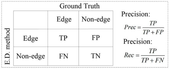
Figure 3.
Confusion matrix for the edge detection problem.
4.3. Evaluation on Artificial Datasets
In practice, two cases make edge detection a challenge. The first one is objects that are embedded by background clutter, and the second is weak edges caused by spectral mixture or just appearing in a small subset of bands. As a result, we constructed two artificial images, AI 1 and AI 2, to evaluate the performance of our proposed edge detection approach under these two cases.
A. Experiment on AI 1
In this experiment, we investigated the behaviors of the five edge-detection methods when the objects in an image are embedded by background clutter. The tested image AI 1 is composed of one object (in the middle) and a background, where the object is located between column 60 and column 120. Thus, edge pixels are located at columns 60 and 120. To simulate different levels of background clutter, we added Gaussian noises with various Signal Noise Ratio (SNR) to AI 1. The object noise is fixed to SNR = 16 dB, whereas the background noise varies from 0.1 to 3.0 dB. Figure 4a shows the content of the synthetic image without noise. Figure 4b shows a channel for the background with SNR = 0.2 dB.
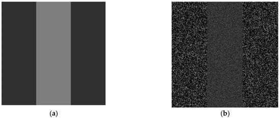
Figure 4.
A channel in the AI 1 dataset: (a) The content of the synthetic image without noise (object is located in the middle); and (b) a corrupted image with SNR = 16 dB (where SNR stands Signal Noise Ratio) in the object region and SNR = 0.2 dB in the background region. The dark color indicates low intensity.
Figure 5 shows an edge-detection example for AI 1, where the background noise is SNR = 0.2 dB. The edge-strength maps and corresponding binary edge maps were shown in the first row and the second row, respectively, in Figure 5. For Di Zenzo’s method, the strength of the edge pixels is slightly larger than the background (Figure 5b). Although we can set a pair of thresholds to separate edge and non-edge pixels, severe false positive detections cannot be avoided, as shown in Figure 5g. For the RCMG, the strength of noisy pixels is larger than that of edge pixels, as shown in Figure 5c; thus, the boundaries of the object were concealed from the noisy background (Figure 5h). According to Figure 5d,i, the results of Drewniok’s method are better than those of Di Zenzo’s and the RCMG method, but they blurred the edges to some extent (Figure 5d). Therefore, the object’s edges were blurred with burrs, as shown in Figure 5i. For the SSSDE, the strength of almost all the edge pixels is larger than that of the noise pixels as depicted in Figure 5e. However, some false edges are detected in the object, as shown in Figure 5j. Compared to the other four methods, the better performance of the presented detector is clearly perceivable, and the strength of the edge pixels is larger than that of the noise pixels (Figure 5a). It is therefore easy to set appropriate thresholds to separate the edge and non-edge pixels, as shown in Figure 5e.
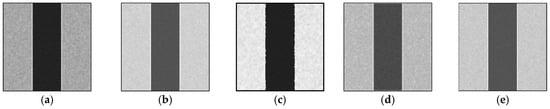
Figure 5.
Edge-strength maps and corresponding binary edges of AI 1 with SNR = 0.2 dB. Edge-strength maps of: (a) GEDHSI; (b) Di Zenzo’s method; (c) the Robust Color Morphological Gradient (RCMG) method; (d) Drewniok’s method; and (e) the modified Simultaneous Spectral/Spatial Detection of Edges (SSSDE) method. (f–j) Binary edge maps of corresponding results of (a–e).
The robustness to the background clutter of the GEDHSI was further demonstrated in Figure 6, under different background-noise levels from 0.1 dB to 3 dB. From Figure 6b we can find that the GEDHSI produces better Rec values in almost all the noise levels. This indicates the successful detection of almost all the edges, which is also confirmed by Figure 5f. Although the Prec values obtained by the GEDHSI are occasionally slightly worse than that of Di Zenzo’s method, it increases quickly as SNR raised as shown in Figure 6a. For the F-measure in Figure 6c, we can see that under high background-noise levels (SNR approximately 0.1 dB), the GEDHSI produced an F-measure value larger than 0.9, whereas the F-measure values produced by the other four methods are all less than 0.7. When the SNR surpasses 0.9, the F-measure value for the GEDHSI reaches approximately 1.0, whereas for the other four methods the F-measure values increased slowly. It is obvious that the other four methods are weaker than the GEDHSI in addressing such severe background clutter. With severe noise interference, the large difference between a noisy pixel and its neighbors usually leads to a high gradient magnitude for that noisy pixel, a magnitude even larger than that of the true edge pixels. As a result, this will inevitably cause incorrect edges because of failing to make the full use of the spatial information of the image, especially inadequate consideration of the relationships among the pixels within a local window.
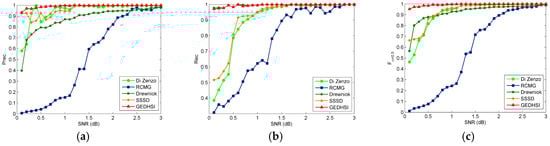
Figure 6.
Performance evaluation on AI 1 under various noise levels. Performance of: (a) Precision; (b) Recall; and (c) F-measure.
B. Experiment on AI 2
In this experiment, we analyze the behaviors of the five edge-detection methods in dealing with weak edges between objects. For HSIs, weak edges are usually caused by spectral mixture between objects or edges appearing in only a small subset of bands [17]. To tackle this problem, we generated a well-designed image AI 2 with a spatial dimension of 180 × 180 in nine regions. The size of each region is 60 × 60 pixels. We first selected three types of endmembers from the USGS Spectral Library [60], as shown in Figure 7a.
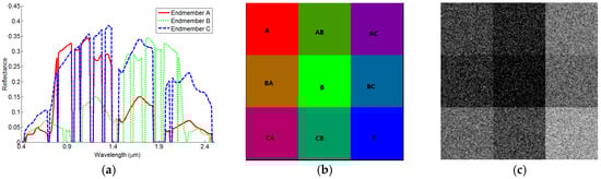
Figure 7.
Materials for AI 2: (a) curve of endmembers; (b) diagram of AI 2; and (c) a band of AI 2 with SNR = 10 dB.
According to Figure 7a, the two endmembers A and C are found to be very similar in the range of 0.6 µm to 1.4 µm, whereas the two endmembers B and C are very similar in the range of 1.5 µm to 2.1 µm. A diagram of AI 2 is shown in Figure 7b, where the symbol of each region denotes which endmembers the region is formed. For example, the “A” of Region A means the region was generated only using endmember A, Region AB was generated by using endmembers A and B, whereas Region BA was composed of endmembers B and A, etc. Except for the three regions located in the principal diagonal, all regions were mixed by different endmembers. The mixed ratio was fixed as 0.4:0.6 for these regions. We then added Gaussian noise to AI 2 and result in a varying SNR between 1 and 30 dB. Figure 7c shows an example band with SNR = 10 dB. Due to the spectral mixture and spectral similarity in many bands, there are several weak edges. Under such conditions, weak edges may be easily vanished in noise when white Gaussian noise was added.
For the noise-degraded AI 2 with a SNR of 10 dB, Figure 8 shows the edge-strength maps (the first row) and their corresponding binary edge maps (the second row) generated by the five methods. As seen from the edge-strength maps generated by Di Zenzo’s method (Figure 8b), the RCMG (Figure 8c), Drewniok’s method (Figure 8d) and SSSDE method (Figure 8e), the strength of upper horizontal and left vertical edge pixels is close to that of the noisy pixels. Therefore, it is difficult to set appropriate thresholds for these edge-strength maps. According to Figure 8g, Di Zenzo’s method seems to produce discontinuous edges and severe false edges. Although RCMG is slightly better than Di Zenzo’s as shown in Figure 8h, the results still contains some spurious edges. The similar problems exist in the results of SSSDE as illustrated in Figure 8j through the SSSDE generate much better results than RCMG. Although Drewniok’s method has removed almost all noise, the edges are hackly due to the displacement caused by Gaussian smoothing in each band. For comparison, the intensity of the edge pixels is dramatically larger than that of the noisy pixels, as shown in Figure 8a. Thus, thresholding can easily classify edge and non-edge pixels, as shown in Figure 8f.
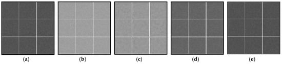
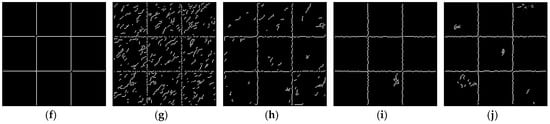
Figure 8.
Edge-strength maps and corresponding binary edges of AI 2 with SNR = 10 dB. Edge-strength maps of: (a) GEDHSI; (b) Di Zenzo’s method; (c) the RCMG method; (d) Drewniok’s method; and (e) SSSDE method. (f–j) Binary edge maps of corresponding results of (a–e) by applying automatic hysteresis thresholding and thinning processes.
Figure 9 shows the performance comparison of the five methods under noise from 1.0 dB to 30 dB. As seen in Figure 9c, due to the simplicity of the tested image, all five methods produced good results when the level of noise is low (SNR > 10 db). With the increase of noise level, especially when SNR < 7 db, the F-measure values of the four compared algorithms decreased rapidly while the proposed GEDHSI still produce much better results. Furthermore, GEDHSI obtained better results on both Prec and Rec values than Di Zenzo’s, RCMG and SSSDE methods as illustrated in Figure 9a,b. This demonstrates the GEDHSI can detect the edges in the HSIs with higher accuracy in the complicated environments. For Drewniok’s method, although its Rec values are better than that of the GEDHSI to some extent, its Prec values are remarkably worse. This implies that Drewniok’s method is easily affected by the noise, which is also confirmed by the F-measure shown in Figure 9c. Moreover, the jagged boundaries between different edges in Figure 8i also confirm that Drewniok’s method produces many false edges. To this end, we can reasonably conclude that GEDHSI is more robust to severe noise and weak edges than the other four methods.
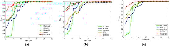
Figure 9.
Performance evaluation on AI 2 under various noise levels: (a) precision; (b) recall; and (c) F-measure.
4.4. Evaluation on Real World Datasets
4.4.1. Experiments on Remote Sensing Datasets
For remote sensing images, due to the complexity of land cover based surface feature, illumination and atmospheric effects as well as spectral mixing of pixels, edges are always deteriorated for proper detection. More seriously, there usually exist some noisy bands in remote sensing HSIs, which make edge detection very difficult. To validate the performance of edge detection on remote sensing HSIs, we selected two remote sensing HSIs, the Farmland and Washington DC Mall image as shown in Figure 10 and Figure 12, to conduct experiments in this section.
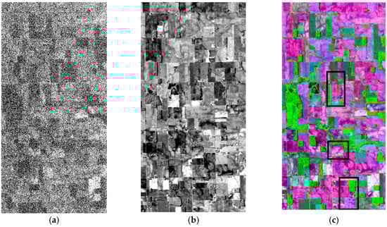
Figure 10.
Farmland image: (a) noisy image in gray-scale (band 1); (b) noiseless image in gray-scale (band 87); and (c) three-band false color composite (bands 25, 60, 128).
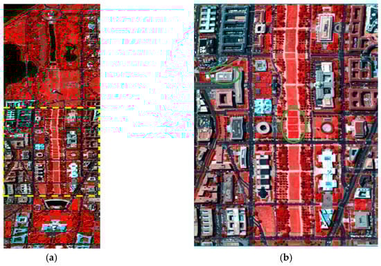
Figure 12.
False color representation of the Washington DC Mall hyperspectral data: (a) the whole data; and (b) the detail display of the doted rectangle region of (a) with two regions emphasized in ellipses to show local tiny structures.
A. Experiment on the Farmland HSIs
Figure 10 is the Farmland image obtained by AVIRIS. The AVIRIS instrument contains 224 different detectors, where the spectral band width is approximately 0.01 µm, allowing it to cover the entire range between 0.4 µm and 2.5 µm. There are several low SNR bands in the AVIRIS image, and one example is shown in Figure 10a where the edges are nearly invisible. Even in some noiseless bands, as shown in Figure 10b, the edges are still very vague. Composited with three low correlation bands, the edge structure can be much clearer as shown in Figure 10c. This is mainly due to the effective utilization of spectral information. In addition, as shown in Figure 10c, the boundaries between regions are clearer, which make it appropriate for the evaluation of edge detection algorithms. However, in the composited image, the pixels inside the region are heavily textured, which makes edge detection a difficult problem.
Figure 11 illustrates the results of edge detection from the four methods. Overall, the better performance of the GEDHSI on the image is clearly perceivable. The proposed GEDHSI has produced continuous, compact and clear edges, where the most edge structures are well preserved as shown in Figure 11a. For Di Zenzo's method, almost all of edges produced are broken as shown in Figure 11b. Drewniok’s method generates many spurious edges within regions and some line edges are distorted at the place where it should be straight according to Figure 11d. RCMG and SSSDE produce similar results as GEDHSI. However, there are many grainy edges with some fine edge structures missing or distorted to some degree, as shown in Figure 11c,e. Specifically, as labeled by the red rectangles, Di Zenzo’s method has detected serious broken edges. Drewniok’s method generates many small and severe spurious edges and fails to capture the main structure. Moreover, Drewniok’s method results in distortion and flexuous edges. The RCMG produces some grainy and slightly distorted edges. In contrast, the edges produced by the proposed GEDHSI are straight and continuous.
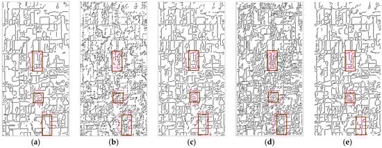
Figure 11.
The binary edge maps of the Farmland image by: (a) GEDHSI; (b) Di Zenzo’s method; (c) the RCMG method; (d) Drewniok’s method (); and (e) SSSDE method.
B. Experiment on the Washington DC Mall HSIs
Figure 12 is an image obtained by HYDICE, which has 210 bands ranging from 0.4 µm to 2.4 µm and covers the visible and (near) infrared spectrum. Bands in the 0.9 µm and 1.4 µm regions where the atmosphere is opaque have been omitted from the dataset, leaving 191 bands for experiments. As shown in Figure 12a, the dataset contains complex and cluttered landcovers. Especially in the middle of Figure 12a, as highlighted within a dotted rectangle, various roofs, roads, trails, grass, trees and shadow are cluttered. For better visual effect, the enlarged version of this part of the image is shown in Figure 12b. This is used for testing as it contains abundant tinny edges which is difficult to be detected completely. Examples of these tiny structures can be found in the two ellipses in Figure 12b, where local details such as the boxes on the roof and the footpath are clearly visible yet hard for detection.
Figure 13 illustrates the edge results for Figure 13b produced by the five methods. According to the criteria of Reference [54], a good detection should keep good edge resolution and connectivity. The superiority of the proposed method on these criteria is clearly visible as shown in Figure 13. The edge image of Di Zenzo’s method is poor and contains many broken edges as shown in Figure 13b. The RCMG and SSSDE are better than Di Zenzo’s method, but they still produce many grainy and spurious edges (Figure 13c,e). Compared with RCMG and SSSDE, the edge map produced by the Drewniok’s method in Figure 13d contains more grainy edges within regions and more spurious edges. In contrast, the edges in Figure 13a produced by our approach are clearer and of better connectivity, where most of fine edge structures from different land covers are successfully detected.
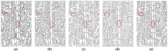
Figure 13.
The binary edge maps of the Washington DC Mall by: (a) GEDHSI; (b) Di Zenzo’s method; (c) the RCMG method; (d) Drewniok’s method ( = 1.0); and (e) SSSDE method.
For the edge resolution criterion, the better performance of the proposed method is also obviously perceivable. In the upper left ellipse of Figure 13b,d, the Di Zenzo’s and RCMG methods have missed the edge structures, while the proposed GEDHSI preserves such tiny structures very well. In the lower right corner ellipse of Figure 13c–e, the RCMG, Drewniok’s, and SSSDE methods not only fail to obtain continuous edge but also miss one side of the edge. On the contrary, the proposed GEDHSI can detect complete edges at both side of the path. Overall, the proposed approach is more effective than the other four methods for detecting edges from these HSIs.
4.4.2. Experiments on Ground Scene Datasets
Both of the two tested real ground scenes images cover the wavelength from 0.4 µm to 0.72 µm, and are sampled at 0.01 µm intervals and result in 31 bands. For simplicity, we selected two images, Scenes 5 and Scenes 7 as illustrated, because of the following two reasons: First, as shown in Figure 14, the spatial resolution is higher than the four other datasets and they contain many man-made objects, thus we know where the edges occur exactly. Therefore, they are rather appropriate for performance evaluation. Second, there are heavily textured objects in the datasets, such as the objects surrounded by a heavily textured wall in Scene 5 (Figure 14a), and finely textured walls and grass in Scene 7 (Figure 14b). Edge detection under these circumstances is still a challenge.
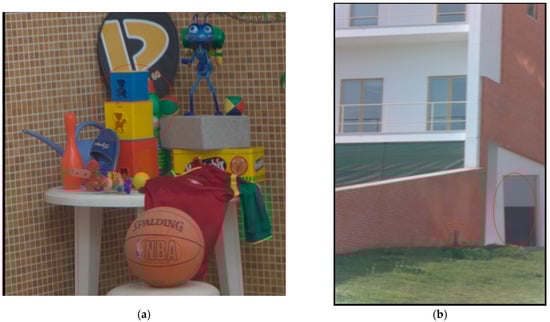
Figure 14.
RGB representations of two hyperspectral scene dataset: (a) Scene 5; and (b) Scene 7.
A. Experiment on the Scene 5 dataset
For the Scene 5 dataset, Figure 15 illustrates the binary edge maps generated by the five methods. Obviously, Di Zenzo’s edge image is poor and contains many small and spurious edges, and the details of the wall are poorly detected as shown in Figure 15b. Compared to Figure 15b, the RCMG method can detect more edges on the wall, while there are still some spurious edges especially on the chair, under the ball and at the bottom right of the wall due to the variance in intensity of the surface as shown in Figure 15c. Drewniok’s method performs better than Di Zenzo’s method on the wall, but it has produced more spurious and grainy edges than either the RCMG or GEDHSI. Some fine edges on the wall grid and racket bag are missing (Figure 15d). Performance of SSSDE is better than that of Di Zenzo’s and Drewniok’s on the left wall, while it misses many edges on the blue and yellow boxes as well as the basketball, as shown in Figure 15e. In contrast, almost complete edges of most objects are attained by the proposed method as shown in Figure 15a. The details in the circle from Figure 15 also illustrate the efficacy of the proposed method, where the proposed GEDHSI method has generated the best edge results in keeping the real structure.
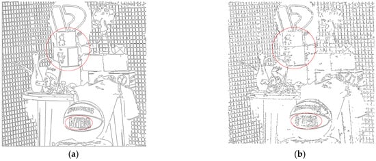
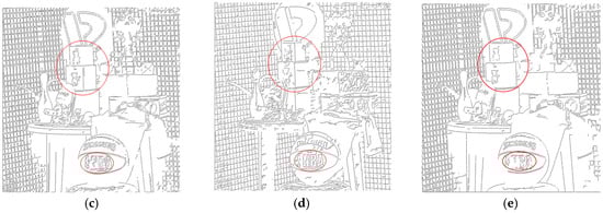
Figure 15.
The binary edge maps generated for the Scene 5 dataset by: (a) GEDHSI; (b) Di Zenzo’s method; (c) the RCMG method; (d) Drewniok’s method ( = 1.0); and (e) SSSDE.
B. Experiment on Scene 7
Figure 16 shows the binary edge maps of Scene 7 produced by the five methods. According to Figure 16b, Di Zenzo’s method produces many spurious edges and performs poorly on connectivity. The RCMG preserves most significant spatial structures, but it also brings many grainy edges especially in the grass region as shown in Figure 16c. The Drewniok’s method can detect many edges on the wall and grass as depicted in Figure 16d, but the interval between edges on the windows is enlarged due to edges displacement caused by Gaussian smoothing. Connectivity of edges generated by SSSDE is better than that of Di Zenzo’s while some edges between the upper and lower windows are missed, as can be seen in Figure 16e. Comparatively, the better performance of the proposed method is perceivable. Most of the fine edge structures such as the edges located at the windows are attained and the edges are clear and connective as shown in Figure 16a. More specifically, as indicated by the circle at the bottom of the image, Di Zenzo’s and Drewniok’s methods produce undesirable edges for the grass in the circle. The RCMG almost misses and the SSSDE totally misses the edge structure. Comparatively, the fine structure is well preserved by the proposed GEDHSI method. At the right bottom ellipse, Drewniok’s method has missed both the edge of the left sidewalls and the edge between the middle white door and the dark shadow. On the contrary, the proposed GEDHSI can again detect correct edges without missing main structure of that region.
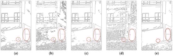
Figure 16.
The binary edge maps generated for the Scene 7 by: (a) GEDHSI; (b) Di Zenzo’s method; (c) the RCMG method; (d) Drewniok’s method ( = 1.0); and (e) SSSDE.
Overall, the comparative experiments above have validated the superiority of the proposed GEDHSI for edge detection in HSIs. The proposed method is more robust to background clusters and weak edges, as illustrated by the experiments on artificial images. For real-world images, it is robust to noisy bands in keeping complete and reasonable spatial structures and performs well on edge localization and resolution. As a result, GEDHSI is more suitable for HSI edge detection than other state-of-the-art multi-band approaches.
4.5. Comparison of Runtime
In this section, we compare the computational efficiency of the above five algorithms. The mean computational time (in seconds) required by each algorithm for five independent runs in solving the two tested images, the Farmland and Washington DC Mall, are presented for comparison.
As seen in Table 2, RCMG takes the least time, and one main reason is its C++ based implementation in comparison to the MATLAB-based implementation for the other four methods. The proposed GEDHSI, unfortunately, consumes the longest runtime as a whole. The long time consumption is largely caused by the iterative computation in traveling procedure. For each particle, the repeating calculation of gravitational force for all particles in dataset D leads to heavy burden of runtime. How to speed up the process and improve the efficiency of GEDHSI will be investigated in the future.
Table 2.
The time efficiency evaluation.
5. Conclusions
In recent years, various heuristic and physically inspired image-understanding methods have been developed. To extract the edges from HSIs, a novel edge-detection method, namely Gravitation-based Edge Detection on HSIs (GEDHSI), is presented in this paper. In GEDHSI, each pixel is modeled as a movable celestial object in the joined spatial-spectral feature space where all objects travel in the feature space under the gravitational field force. Due to the relative positions, the edge pixels and non-edge pixels can be separated by computing their potential energy fields. In addition to its simplicity and generality, GEDHSI has promising theoretical properties that make it a solid tool for edge detection. The performance of the proposed algorithm has been benchmarked with four state-of-the-art methods, including Di Zenzo’s, Drewniok’s, RCMG, and SSSD detectors. Experiments on a variety of datasets have validated the efficacy of the proposed algorithm in edge-detection for HSIs under various levels of noise. The future work will focus on further improving the efficiency of the approach and investigating the relationship between the edge scale and the parameter settings for edge results in the multiscale space.
Acknowledgments
This work was supported by Chinese Natural Science Foundation Projects (41471353) and National Key Research and Development Program of China (2016YFB0501501).
Author Contributions
Genyun Sun, Aizhu Zhang, and Peng Wang conceived, designed and performed the experiments, analyzed the data, and wrote the paper. Jinchang Ren, Jingsheng Ma, and Yuanzhi Zhang help organize and revise the paper. Xiuping Jia helps analyze the experimental data and improve the presentation of the second version.
Conflicts of Interest
The authors declare no conflict of interest.
References
- Tarabalka, Y.; Benediktsson, J.A.; Chanussot, J. Spectral-spatial classification of hyperspectral imagery based on partitional clustering techniques. IEEE Trans. Geosci. Remote Sens. 2009, 47, 2973–2987. [Google Scholar] [CrossRef]
- Youn, S.; Lee, C. Edge Detection for Hyperspectral Images Using the Bhattacharyya Distance. In Proceedings of the 2013 International Conference on Parallel and Distributed Systems, Seoul, South Korea, 15–18 December 2013; pp. 716–719. [Google Scholar]
- Kiani, A.; Sahebi, M.R. Edge detection based on the Shannon Entropy by piecewise thresholding on remote sensing images. IET Comput. Vis. 2015, 9, 758–768. [Google Scholar] [CrossRef]
- Weng, Q.; Quattrochi, D.A. Urban Remote Sensing; CRC Press: Boca Raton, FL, USA, 2006. [Google Scholar]
- Canny, J. A computational approach to edge detection. IEEE Trans. Pattern Anal. Mach. Intell. 1986, PAMI-8, 679–698. [Google Scholar] [CrossRef]
- Marr, D.; Hildreth, E. Theory of edge detection. Proc. R. Soc. Lond. B Biol. Sci. 1980, 207, 187–217. [Google Scholar] [CrossRef] [PubMed]
- Smith, S.M.; Brady, J.M. SUSAN—A new approach to low level image processing. Int. J. Comput. Vis. 1997, 23, 45–78. [Google Scholar] [CrossRef]
- Chan, T.F.; Vese, L.A. Active contours without edges. IEEE Trans. Image. Process. 2001, 10, 266–277. [Google Scholar] [CrossRef] [PubMed]
- Priego, B.; Souto, D.; Bellas, F.; Duro, R.J. Hyperspectral image segmentation through evolved cellular automata. Pattern Recogn. Lett. 2013, 34, 1648–1658. [Google Scholar] [CrossRef]
- Tarabalka, Y.; Chanussot, J.; Benediktsson, J.A. Segmentation and classification of hyperspectral images using watershed transformation. Pattern Recogn. 2010, 43, 2367–2379. [Google Scholar] [CrossRef]
- Bakker, W.; Schmidt, K. Hyperspectral edge filtering for measuring homogeneity of surface cover types. ISPRS J. Photogramm. 2002, 56, 246–256. [Google Scholar] [CrossRef]
- Kanade, T. Image Understanding Research at CMU. Available online: http://oai.dtic.mil/oai/oai?verb=getRecord&metadataPrefix=html&identifier=ADP000103 (accessed on 28 March 2017).
- Hedley, M.; Yan, H. Segmentation of color images using spatial and color space information. J. Electron. Imaging 1992, 1, 374–380. [Google Scholar] [CrossRef]
- Fan, J.; Yau, D.K.; Elmagarmid, A.K.; Aref, W.G. Automatic image segmentation by integrating color-edge extraction and seeded region growing. IEEE Trans. Image Process. 2001, 10, 1454–1466. [Google Scholar] [PubMed]
- Garzelli, A.; Aiazzi, B.; Baronti, S.; Selva, M.; Alparone, L. Hyperspectral image fusion. In Proceedings of the Hyperspectral 2010 Workshop, Frascati, Italy, 17–19 March 2010. [Google Scholar]
- Lei, T.; Fan, Y.; Wang, Y. Colour edge detection based on the fusion of hue component and principal component analysis. IET Image Process. 2014, 8, 44–55. [Google Scholar] [CrossRef]
- Di Zenzo, S. A note on the gradient of a multi-image. Comput. Vis. Graph. Image Process. 1986, 33, 116–125. [Google Scholar] [CrossRef]
- Cumani, A. Edge detection in multispectral images. CVGIP Graph. Model. Image Process. 1991, 53, 40–51. [Google Scholar] [CrossRef]
- Drewniok, C. Multi-spectral edge detection. Some experiments on data from Landsat-TM. Int. J. Remote Sens. 1994, 15, 3743–3765. [Google Scholar] [CrossRef]
- Jin, L.; Liu, H.; Xu, X.; Song, E. Improved direction estimation for Di Zenzo’s multichannel image gradient operator. Pattern Recogn. 2012, 45, 4300–4311. [Google Scholar] [CrossRef]
- Trahanias, P.E.; Venetsanopoulos, A.N. Color edge detection using vector order statistics. IEEE Trans. Image Process. 1993, 2, 259–264. [Google Scholar] [CrossRef] [PubMed]
- Toivanen, P.J.; Ansamäki, J.; Parkkinen, J.; Mielikäinen, J. Edge detection in multispectral images using the self-organizing map. Pattern Recogn. Lett. 2003, 24, 2987–2994. [Google Scholar] [CrossRef]
- Haralick, R.M.; Sternberg, S.R.; Zhuang, X. Image analysis using mathematical morphology. IEEE Trans. Pattern. Anal. Mach. Intell. 1987, PAMI-9, 532–550. [Google Scholar] [CrossRef]
- Evans, A.N.; Liu, X.U. A morphological gradient approach to color edge detection. IEEE Trans. Image Process. 2006, 15, 1454–1463. [Google Scholar] [CrossRef] [PubMed]
- Lopez-Molina, C.; De Baets, B.; Bustince, H. Quantitative error measures for edge detection. Pattern Recogn. 2013, 46, 1125–1139. [Google Scholar] [CrossRef]
- Wang, Y.; Niu, R.; Yu, X. Anisotropic diffusion for hyperspectral imagery enhancement. IEEE Sens. J. 2010, 10, 469–477. [Google Scholar] [CrossRef]
- Dinh, C.V.; Leitner, R.; Paclik, P.; Loog, M.; Duin, R.P. SEDMI: Saliency based edge detection in multispectral images. Image Vis. Comput. 2011, 29, 546–556. [Google Scholar] [CrossRef]
- Fossati, C.; Bourennane, S.; Cailly, A. Edge Detection Method Based on Signal Subspace Dimension for Hyperspectral Images; Springer: New York, NY, USA, 2015. [Google Scholar]
- Paskaleva, B.S.; Godoy, S.E.; Jang, W.Y.; Bender, S.C.; Krishna, S.; Hayat, M.M. Model-Based Edge Detector for Spectral Imagery Using Sparse Spatiospectral Masks. IEEE Trans. Image Process. 2014, 23, 2315–2327. [Google Scholar] [CrossRef] [PubMed]
- Resmini, R.G. Simultaneous spectral/spatial detection of edges for hyperspectral imagery: the HySPADE algorithm revisited. In Proceedings of the SPIE Defense, Security, and Sensing International Society for Optics and Photonics, Baltimore, MD, USA, 23–27 April 2012; Volume 83930. [Google Scholar]
- Resmini, R.G. Hyperspectral/spatial detection of edges (HySPADE): An algorithm for spatial and spectral analysis of hyperspectral information. In Proceedings of the SPIE—The International Society for Optical Engineering, Orlando, USA, 12–16 April 2004; Volume 5425, pp. 433–442. [Google Scholar]
- Lin, Z.; Jiang, J.; Wang, Z. Edge detection in the feature space. Image Vis. Comput. 2011, 29, 142–154. [Google Scholar] [CrossRef]
- Jia, X.; Richards, J. Cluster-space representation for hyperspectral data classification. IEEE Trans. Geosci. Remote Sens. 2002, 40, 593–598. [Google Scholar]
- Imani, M.; Ghassemian, H. Feature space discriminant analysis for hyperspectral data feature reduction. ISPRS J. Photogramm. 2015, 102, 1–13. [Google Scholar] [CrossRef]
- Gomez-Chova, L.; Calpe, J.; Camps-Valls, G.; Martin, J.; Soria, E.; Vila, J.; Alonso-Chorda, L.; Moreno, J. Feature selection of hyperspectral data through local correlation and SFFS for crop classification. In Proceedings of the Geoscience and Remote Sensing Symposium, Toulouse, France, 21–25 July 2003; Volume 1, pp. 555–557. [Google Scholar]
- Zhang, Y.; Wu, K.; Du, B.; Zhang, L.; Hu, X. Hyperspectral Target Detection via Adaptive Joint Sparse Representation and Multi-Task Learning with Locality Information. Remote Sens. 2017, 9, 482. [Google Scholar] [CrossRef]
- Rashedi, E.; Nezamabadi-Pour, H. A stochastic gravitational approach to feature based color image segmentation. Eng. Appl. Artif. Intell. 2013, 26, 1322–1332. [Google Scholar] [CrossRef]
- Sen, D.; Pal, S.K. Improving feature space based image segmentation via density modification. Inf. Sci. 2012, 191, 169–191. [Google Scholar] [CrossRef]
- Peters, R.A. A new algorithm for image noise reduction using mathematical morphology. IEEE Trans. Image Process. 1995, 4, 554–568. [Google Scholar] [CrossRef] [PubMed]
- Perona, P.; Malik, J. Scale-space and edge detection using anisotropic diffusion. IEEE Trans. Pattern Anal. 1990, 12, 629–639. [Google Scholar] [CrossRef]
- Olenick, R.P.; Apostol, T.M.; Goodstein, D.L. The Mechanical Universe: Introduction to Mechanics and Heat; Cambridge University Press: Cambridge, UK, 2008. [Google Scholar]
- Sun, G.Y.; Zhang, A.Z.; Yao, Y.J.; Wang, Z.J. A novel hybrid algorithm of gravitational search algorithm with genetic algorithm for multi-level thresholding. Appl. Soft Comput. 2016, 46, 703–730. [Google Scholar] [CrossRef]
- De Mesquita Sá Junior, J.J.; Ricardo Backes, A.; César Cortez, P. Color texture classification based on gravitational collapse. Pattern Recogn. 2013, 46, 1628–1637. [Google Scholar] [CrossRef]
- Peng, L.; Yang, B.; Chen, Y.; Abraham, A. Data gravitation based classification. Inf. Sci. 2009, 179, 809–819. [Google Scholar] [CrossRef]
- Cano, A.; Zafra, A.; Ventura, S. Weighted data gravitation classification for standard and imbalanced data. IEEE Trans. Cybern. 2013, 43, 1672–1687. [Google Scholar] [CrossRef] [PubMed]
- Peng, L.; Zhang, H.; Yang, B.; Chen, Y. A new approach for imbalanced data classification based on data gravitation. Inf. Sci. 2014, 288, 347–373. [Google Scholar] [CrossRef]
- Ilc, N.; Dobnikar, A. Generation of a clustering ensemble based on a gravitational self-organising map. Neurocomputing 2012, 96, 47–56. [Google Scholar] [CrossRef]
- Lopez-Molina, C.; Bustince, H.; Fernández, J.; Couto, P.; De Baets, B. A gravitational approach to edge detection based on triangular norms. Pattern Recogn. 2010, 43, 3730–3741. [Google Scholar] [CrossRef]
- Sun, G.; Liu, Q.; Liu, Q.; Ji, C.; Li, X. A novel approach for edge detection based on the theory of universal gravity. Pattern Recogn. 2007, 40, 2766–2775. [Google Scholar] [CrossRef]
- Rashedi, E.; Nezamabadi-Pour, H.; Saryazdi, S. GSA: A gravitational search algorithm. Inf. Sci. 2009, 179, 2232–2248. [Google Scholar] [CrossRef]
- Sretenskii, L.N. Theory of the Newton Potential; Moscow-Leningrad: Moskva, Russia, 1946. [Google Scholar]
- Hulthén, L.; Sugawara, M. Encyclopaedia of Physics; Springer: Berlin, Germany, 1957; Volume 39. [Google Scholar]
- Medina-Carnicer, R.; Munoz-Salinas, R.; Yeguas-Bolivar, E.; Diaz-Mas, L. A novel method to look for the hysteresis thresholds for the Canny edge detector. Pattern Recogn. 2011, 44, 1201–1211. [Google Scholar] [CrossRef]
- Shui, P.L.; Zhang, W.C. Noise-robust edge detector combining isotropic and anisotropic Gaussian kernels. Pattern Recogn. 2012, 45, 806–820. [Google Scholar] [CrossRef]
- Rink, T.; Antonelli, P.; Whittaker, T.; Baggett, K.; Gumley, L.; Huang, A. Introducing HYDRA: A multispectral data analysis toolkit. Bull. Am. Meteorol. Soc. 2007, 88, 159–166. [Google Scholar] [CrossRef]
- Green, R.O.; Eastwood, M.L.; Sarture, C.M.; Chrien, T.G.; Aronsson, M.; Chippendale, B.J.; Faust, J.A.; Pavri, B.E.; Chovit, C.J.; Solis, M. Imaging spectroscopy and the airborne visible/infrared imaging spectrometer (AVIRIS). Remote Sens. Environ. 1998, 65, 227–248. [Google Scholar] [CrossRef]
- Landgrebe, D. Hyperspectral image data analysis. IEEE Signal Process. Mag. 2002, 19, 17–28. [Google Scholar] [CrossRef]
- Foster, D.H. Hyperspectral Images of Natural Scenes 2002. Available online: http://personalpages.manchester.ac.uk/staff/d.h.foster/Hyperspectral_images_of_natural_scenes_02.html (accessed on 10 June 2017).
- González-Hidalgo, M.; Massanet, S.; Mir, A.; Ruiz-Aguilera, D. On the pair uninorm-implication in the morphological gradient. In Computational Intelligence; Madani, K., Correia, A.D., Rosa, A., Filipe, J., Eds.; Springer: Cham, Switzerland, 2015; Volume 577, pp. 183–197. [Google Scholar]
- Clark, R.N.; Swayze, G.A.; Wise, R.; Livo, K.E.; Hoefen, T.M.; Kokaly, R.F.; Sutley, S.J. USGS Digital Spectral Library Splib06a; USGS: Reston, VA, USA, 2007. [Google Scholar]
© 2017 by the authors. Licensee MDPI, Basel, Switzerland. This article is an open access article distributed under the terms and conditions of the Creative Commons Attribution (CC BY) license (http://creativecommons.org/licenses/by/4.0/).