
Simulation of Ship-Track versus Satellite-Sensor Differences in Oceanic Precipitation Using an Island-Based Radar


1
Department of Earth Sciences, Meteorological Institute, Faculty of Mathematics, Informatics and Natural Sciences, Universität Hamburg, Bundesstraße 55, 20146 Hamburg, Germany
2
Max Planck Institute for Meteorology, Bundesstraße 53, 20146 Hamburg, Germany
*
Author to whom correspondence should be addressed.
Remote Sens. 2017, 9(6), 593; https://doi.org/10.3390/rs9060593
Submission received: 4 April 2017
/
Revised: 18 May 2017
/
Accepted: 8 June 2017
/
Published: 11 June 2017
(This article belongs to the Special Issue Remote Sensing Precipitation Measurement, Validation, and Applications)
Abstract
:The point-to-area problem strongly complicates the validation of satellite-based precipitation estimates, using surface-based point measurements. We simulate the limited spatial representation of light-to-moderate oceanic precipitation rates along ship tracks with respect to areal passive microwave satellite estimates using data from a subtropical island-based radar. The radar data serves to estimate the discrepancy between point-like and areal precipitation measurements. From the spatial discrepancy, two statistical adjustments are derived so that along-track precipitation ship data better represent areal precipitation estimates from satellite sensors. The first statistical adjustment uses the average duration of a precipitation event as seen along a ship track, and the second adjustment uses the median-normalized along-track precipitation rate. Both statistical adjustments combined reduce the root mean squared error by 0.24 mm h (55%) compared to the unadjusted average track of 60 radar pixels in length corresponding to a typical ship speed of 24–34 km h depending on track orientation. Beyond along-track averaging, the statistical adjustments represent an important step towards a more accurate validation of precipitation derived from passive microwave satellite sensors using point-like along-track surface precipitation reference data.
1. Introduction
The validation of satellite-based precipitation estimates using surface-based point measurements is substantially hampered by the long-standing point-to-area (p2a) problem [1,2,3]. The p2a problem mainly arises from the different representation of precipitation in measurements of spatially different resolutions. Differing spatial representations pose a considerably larger challenge for precipitation due to its high spatiotemporal variability and intermittency compared to other atmospheric parameters (e.g., temperature) [4]. A meaningful validation of precipitation estimates derived from satellite sensors requires the different spatial representation of precipitation in point-like surface reference data to be properly addressed—a main goal of this study.
Over continental areas, a number of interpolation methods such as kriging or inverse distance weighting exist to make point measurements of precipitation representative of larger areas, provided that a sufficiently large number of station data is available [2,5,6]. Since a variety of precipitation-measuring instruments have become available, triple collocation is increasingly applied for validation purposes (e.g., [7]). However, triple collocation requires three independent high-quality data sources. In contrast to precipitation over land areas for which triple collocation leads to satisfying results [8], the ocean lacks a dense coverage of frequent, high-quality precipitation data [9]. This lack of information for oceanic precipitation calls for an alternative way to address the p2a problem. This study addresses the p2a problem with the aim of simulating the different spatial representation of precipitation along ship tracks compared to areal satellite estimates, and proposes a p2a adjustment.
As one main contributor to surface precipitation validation data sets over the ocean, the Ocean Rainfall And Ice-phase precipitation measurement Network (OceanRAIN; [10]) provides data from ocean-applicable optical disdrometers deployed on research vessels. In the case of a moving ship, the p2a problem simplifies into a track-to-area problem in which the along-track averaged ship track better represents the area of a satellite pixel compared to single point measurements.
Many satellite-based precipitation estimates partly or entirely rely on passive microwave (PMW) sensors due to their more direct physical relation to precipitation compared to visible and infrared sensors [11]. However, PMW sensors have a rather coarse spatial resolution of several tens of kilometers in diameter that strongly adds to the p2a problem [12].
Simulating the effect of different spatial resolution on precipitation estimates requires a data set that combines high spatial resolution with wide areal coverage. Both requirements are met by weather radars, with their relatively high spatial resolution of about 1 km and their wide areal coverage that usually exceeds 100 km in diameter. Simulations of p2a collocations exist over the Baltic Sea based on radar reflectivity [13]. However, the p2a problem has never been addressed explicitly in a simulation with radar data beyond the combination of precipitation events [14].
To explicitly study the p2a problem and the influence of resolution on precipitation measurements, the island-based S-Band Polarimetric (S-Pol; [15]) radar by the National Center for Atmospheric Research (NCAR) suits well. The S-Pol was deployed on the Caribbean island of Barbuda during the Rain In Cumulus clouds over the Ocean (RICO; [16]) campaign. The conditions during RICO favor the comparison of precipitation along simulated ship tracks with simulated satellite pixels for two reasons. First, RICO contains a high fraction of time with precipitation of predominantly low intensity observed by the S-Pol radar [17]. This means that heavy rainfall has not been sampled by the S-Pol radar data. Second, the climatic conditions in the trades with usually small-scale showers challenge both the realistic representation of precipitation along ship tracks and the overall detection limitations of precipitation within a rather large satellite pixel [18]. Thus, the S-Pol data collected during RICO is well-suited to the investigation of the influence of spatial resolution on the measurement of oceanic precipitation.
We employ the following method: the S-Pol radar data serves to simulate both along-track ship measurements and PMW satellite pixels. Comparing them enables the derivation of statistical adjustments to make the ship data more representative of PMW data. The adjustments need to be solely based on information available from along-track precipitation rates because the sub-pixel variability is usually unknown for satellite-derived precipitation estimates. The p2a-adjusted precipitation rates could ideally be used for various validation purposes involving precipitation data sets that strongly differ in spatial resolution.
The paper is structured as follows: Section 2 introduces the S-Pol radar and the simulation framework. Section 3 consists of three parts: (i) along-track detection of precipitation; (ii) along-track representation of precipitation rate and (iii) deriving track-to-area adjustments. Section 4 presents conclusions and an outlook.
2. Data and Methods
Island-based weather radars offer a good opportunity to investigate the influence of spatial resolution on the estimated precipitation rate over the ocean. They can help to simulate the representation of precipitation using spatial up-scaling. For this study, we choose a radar that was deployed on the small island of Barbuda at 17.61 N and 61.82 W in the tropical North Atlantic with a high oceanic area fraction. Section 2.1 describes the radar, followed by a methodological overview in Section 2.2.
2.1. The S-Pol Radar
The S-Pol radar developed by NCAR provides a cost-effective portable weather radar, used in a variety of field campaigns [15,19]. Among these campaigns was the RICO campaign [16], during which the scanning S-Pol radar operated from 24 November 2004 to 25 January 2005. During RICO, the S-Pol performed surveillance scans with 10.68 cm wavelength at a 0.5 elevation angle, covering a 150 km domain in radius. Each scan was gridded onto a polar grid with a range resolution of 150 m, and underwent extensive filtering to exclude anomalous returns from ground clutter. A minimum reflectivity threshold of 7 dBZ serves to exclude Bragg scattering [20]. The Z–R relationship to convert the measured radar reflectivity Z (dBZ) into a rain rate R (mm h) is
Equation (1) is derived by [21] from particle size distributions measured during RICO aircraft flights. The minimum reflectivity threshold of 7 dBZ corresponds to about 0.19 mm h, which lies below the lowest resolvable precipitation rate for most satellite sensors. Thus, although this threshold of the chosen Z–R relation influences the raining area, absolute precipitation rate differences are negligible for the purposes of this study. The S-Pol data is freely accessible online [22].
2.2. The Simulation Framework
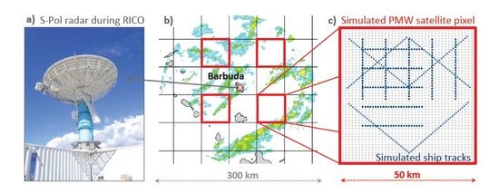
The polar grid of the S-Pol radar consists of 984 range gates and 540 azimuthal increments that represent 0.66 sectors of a circle. The arc length of these azimuthal increments increases with distance from the radar location. This inconstant spatial resolution could distort a spatial-scale comparison. To homogenize the spatial resolution, we brought the S-Pol radar data onto a Cartesian grid with a spatial resolution of about 0.4 km using the nearest-neighbor remapping remapnn of the Climate Data Operators (CDO; [23]). Compared to the size of a PMW satellite pixel of about 50 km × 50 km, 132 × 138 S-Pol radar pixels fill each simulated satellite pixel. In other words, one single radar pixel covers about 0.006% of a simulated satellite pixel and can thus be considered as a point measurement in a satellite pixel. In the scanned area around the radar, we chose four boxes of the typical size of a satellite pixel despite its rather circular shape in reality (Figure 1). These four boxes fulfill the following three conditions.
First, they do not contain any islands in order to avoid land influences. Second, all boxes have about the same medium distance from the radar location. A not-too-large distance from the radar matters to reduce losses by radar beam overshooting above precipitating low clouds. Third, the four boxes are evenly distributed around the radar location to reduce influences of precipitating clouds that align with the prevailing easterly winds [24]. For these reasons, the locations of the four boxes with respect to the radar are well-suited to the study of the effects of spatial-scale differences of precipitation observations.
The whole RICO period spans 62 days (December 2004–January 2005), from which 3662 radar images are available from S-Pol surveillance scans. For the four chosen boxes, this RICO sample results in overall 14,648 simulated satellite pixels. Within these simulated satellite pixels, we chose 16 arbitrary sets of aligned radar pixels for each time step of the S-Pol radar in order to simulate the ship tracks (Figure 1c). From these 16 tracks per box and time step, five align parallel to longitude (lon tracks), five parallel to latitude (lat tracks), and six diagonal with respect to the box. These various orientations rule out biases caused by prevailing cloud directional organization within the box. Assuming a constant ship speed, we chose 24 km h (approx. 13 kn) as a typical ship speed that corresponds to a distance of 0.4 km (one radar pixel) per minute for lon/lat tracks. A one-hour time integration yields track lengths of 24 km for lon/lat tracks and of km for diagonally-oriented tracks, both consisting of 60 radar pixels each.
Along the ship track, we assumed that the precipitation field remains constant with time (i.e., no cloud movement), which markedly differs from reality. However, this assumption should not introduce a bias when considering a sufficiently large number of S-Pol radar images and varying track orientations (cf. Figure 1c). This simplification allows us to use one single S-Pol radar image per simulated satellite pixel and ship track.
By spatial averaging, we obtained two sub datasets from the S-Pol. First, all radar pixels along each of the 16 tracks per box were averaged to obtain a single mean precipitation rate that represents the whole simulated track. Second, all S-Pol radar pixels per box were averaged to represent the simulated satellite-pixel precipitation rate. This framework sets the ground for an independent statistical analysis to study the influence of different spatial resolutions on the measured precipitation rate.
2.3. Weather Conditions during RICO
The RICO period was mainly characterized by frequently occurring light rain events [17,25]. Light rain usually originates from small convective cumulus clouds that are kept shallow by the trade inversion. However, few hours of more widespread precipitation from organized tropical systems complement the otherwise steady conditions during the RICO period.
3. Results
Generally, the high spatiotemporal variability and the intermittency of precipitation complicate its detection and the realistic representation for a sequence of precipitation measurements along a ship track. First, we investigate how well a ship track can detect precipitation compared to the typical area of a PMW satellite sensor, using the available S-Pol radar data from RICO (Section 3.1). Second, we analyze how well a ship track can represent the precipitation rate in a typical area of a PMW satellite sensor (Section 3.2). Third, we propose adjustments so that a precipitation rate along a ship track better represents that of a PMW satellite pixel (Section 3.3). Because the S-Pol radar only sampled rainfall during RICO, we henceforth refer to “rainfall” instead of precipitation.
3.1. Detection of Precipitation along Ship Tracks
Above all, a precipitation observation needs to reliably detect precipitation. Along a ship track, the detection of precipitation mainly depends on two influencing factors.
First, the organization of raining cloud patterns governed by the underlying weather conditions shapes the spatial rainfall distribution within an area. The more homogeneously distributed over the area, the more likely an along-track observation captures the rainfall. During RICO, most rainfall originated from shallow cumulus clouds with a majority not exceeding 1 mm h. The predominantly light rainfall was partially accompanied by more widespread convective rainfall less than 5% of the time [17,25].
Second, the sampling frequency of the individual along-track measurements determines how finely rainfall patterns can be resolved. A lower sampling frequency results in a coarser spatial resolution that might lead to rain events not being captured or dry patterns being erroneously interpreted as rain. Thus, a sampling frequency which is too low can distort parameters such as the rain occurrence. In this simulation study, the sampling is defined by the S-Pol radar resolution and the simulation framework, as explained in Section 2.2. With a more than 100 times higher spatial resolution than the simulated satellite pixel, the simulated along-track measurement sampling provided by the S-Pol radar meets the requirements to investigate the influence of different spatial resolution on the rain rate.
For the rain detection to check how often a simulated ship track misses rain with respect to a simulated satellite pixel, the number of rainy ship tracks is compared to the number of rainy satellite pixels. For both ship tracks and satellite pixels, “rainy” means that from the underlying radar pixels at least one holds a rain rate greater than 0 so that the average rain rate is also greater than 0. From now on, we refer to the simulated satellite pixel as “area” (index A) and to the simulated ship track as “track” (index T). The rain coverage C denotes the fraction of rainy pixels from all pixels along the track () or within the area ().
Considering the 234,368 available cases (i.e., 3662 radar images times 4 simulated satellite pixels times 16 simulated ship tracks), in almost four out of five cases, the area contained rain ( > 0). However, in less than one out of five cases, the track and the area both detected rain, while in more than three out of five cases, the track missed the rainfall observed in the area (Table 1).
The more than three times higher number of rainfall misses compared to rainfall hits points at a poor representation of areal rainfall by the tracks. However, the partial area covered with rain (area rain coverage: ) strongly influences the hit–miss ratio between track and area. Setting to zero below a minimum of 0.01% leads to a hit–miss ratio of 0.28, while a minimum of 1% leads to a hit–miss ratio of 0.6 (for %: 2.4, Figure 2). This relation indicates that the hit–miss ratio of observable rain from tracks with respect to area scales with the minimum area rain coverage. The hit fraction increases with increasing minimum area rain coverage because very small rain events tend to get excluded, which are the most challenging to capture along a track.
An earlier study by [17] revealed for the Northeast radar domain of the same S-Pol radar over Barbuda that the Hamburg Ocean Atmosphere Parameters and Fluxes from satellite (HOAPS; [26,27]) scan-based data (HOAPS-S) can detect some of the rainfall in S-Pol match-ups with an area rain coverage between 1% and 2%, whereas HOAPS certainly detects rainfall above 2% area rain coverage by the S-Pol. Applying this threshold of > 2% leaves 74,544 out of 184,016 rainy cases, while the hit–miss ratio increases from 0.28 to 0.8 (Table 1 and Figure 2). In 3716 cases, the along-track rain coverage exceeds 2% while the area rain coverage does not exceed the minimum threshold of = 2%, and in 5930 cases vice versa. These strongly differing rain-coverage representations also put their mark on the overall rain-rate representation.
3.2. Rain-Rate Representation along Simulated Ship Tracks
For the overall rain-rate representation, both the rain coverage and the rain intensity determine how well the track represents the area. We concentrate on only those 40,538 (17%) cases of all 234,368 cases in which area and track both contain at least one rainy S-Pol radar pixel ( > 0 and > 0 in Table 1). In these “hit cases”, the track might represent the average rain rate differently compared to the area. As a consequence of the non-Gaussian rain-rate distribution, mainly low absolute differences occur between the average along-track rain rate and the average area rain rate . The ratio can serve to estimate how well can represent . As R is composed of the rain coverage and the conditional rain rate of all rainy pixels as , we can determine how C and D contribute to a deviation (Figure 3; 1-by-1 line marks the strongest contribution to deviation). For overestimated along-track rain rates of > 10, the rain coverage C contributes more strongly to the deviation compared to the conditional rain rate D. For an underestimated along-track rain rate of 0.01 < < 0.1, D contributes more strongly to the deviation compared to C until both C and D contribute about equally for < 0.01. For cases of ≈ 1, the track slightly overestimates the rain coverage in the area while the track slightly underestimates the conditional rain rate in the area. Two reasons can explain this behavior. First, the non-Gaussian right-skewed frequency distribution of rain rates causes the track to undersample the rarely occurring most-intense rain-rate pixels that, however, mainly contribute to the conditional rain rate. Second, if the track contains at least a single rainy radar pixel (non-rainy cases excluded in Figure 3), the area is more likely to be over- than undersampled—in particular for low . These statistical features of the rain-rate distribution need to be considered in a potential adjustment of along-track rain rates towards area rain rates.
3.3. Proposed Statistical Track-to-Area Adjustment
The validation of areal data using track-like data demands an adjustment to diminish the track-to-area difference in rain rate. Except for the along-track rain rate, there usually exists no data for the rainfall variability within the satellite pixel to be validated. This lack of spatial information restricts the available information exclusively to the track. However, the track contains an incomplete subsample of the whole area. Therefore, only a statistical parameter of the track derived from a large number of samples can serve to represent information of the spatial rainfall structure within the area. The spatial along-track rainfall structure is composed of the number of sampled rain events per track, , and their individual event duration, , whereby an event marks the longest sequence of rainy pixels uninterrupted by non-rainy pixels. The sum of the duration of all individual rain events along a single track divided by their number yields the average event duration, .
We chose as statistical parameter because can represent the duration of an average rain event as seen along the track. This average rain event duration links to the spatial rainfall structure along the track that ideally conforms to that of the area for a sufficiently large sample size. This relationship between average event duration and actual rain distribution in the area mainly depends on how the rain showers are distributed in the area, as well as their shape. The more homogeneously distributed and uniformly shaped, the better the average event duration can represent the spatial rain distribution of the area.
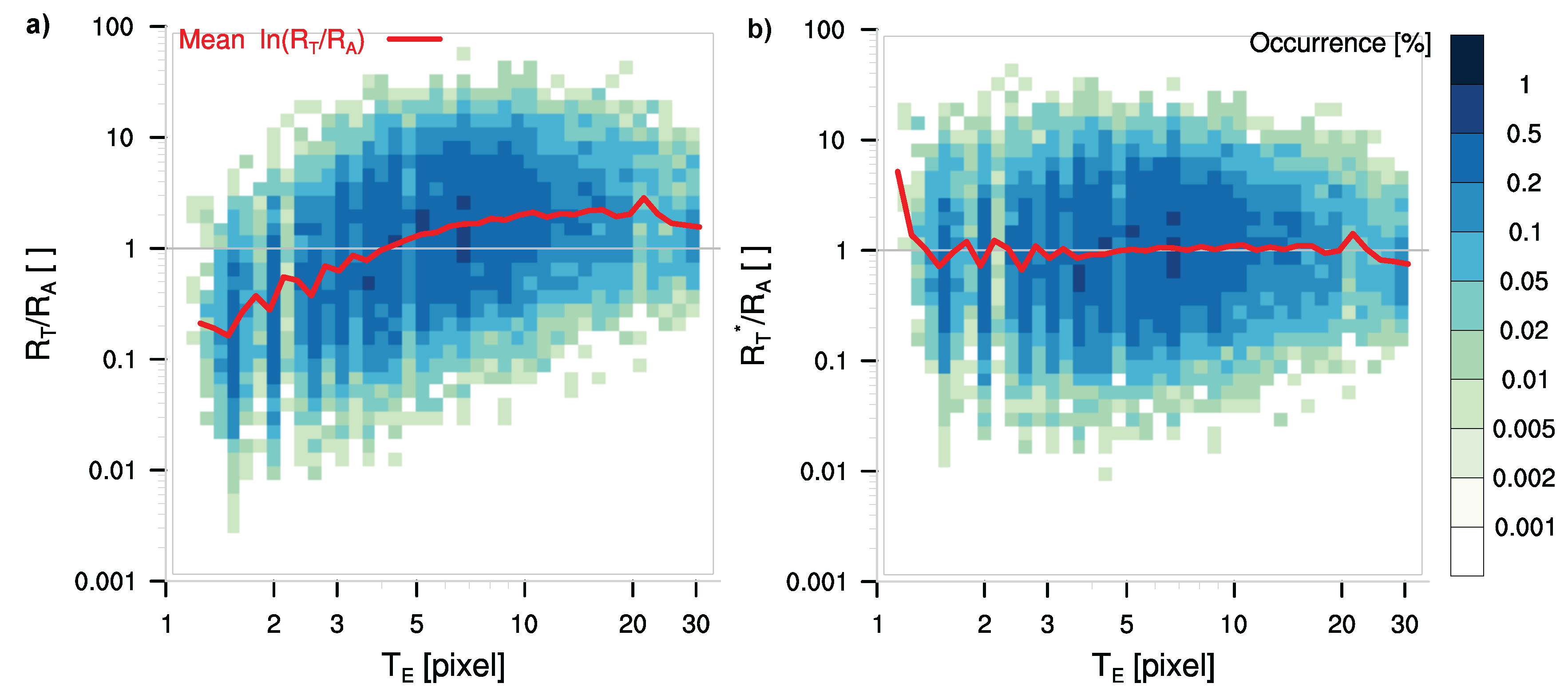
The average event duration revisits the statistical finding of Section 3.2 that the track—on average—overestimates the rain coverage while it underestimates the conditional rain rate (cf. Figure 3). For an average event duration below four radar pixels, underestimates by a factor of two to five (Figure 4). For an average event duration exceeding six radar pixels, approaches a constant overestimation of by a factor of about two. The underestimated rain rate for short events mainly results from the underestimated conditional rain rate along the track with respect to the area. The overestimated rain rate for long-lasting events mainly results from the overestimated rain coverage along the track with respect to the area (not shown). Both effects originate from the limited representativeness of rain along a track within an area.
The deviation of the along-track rain rate from the area rain rate (Figure 4a) can be approximated using an exponential fit for of the following kind:
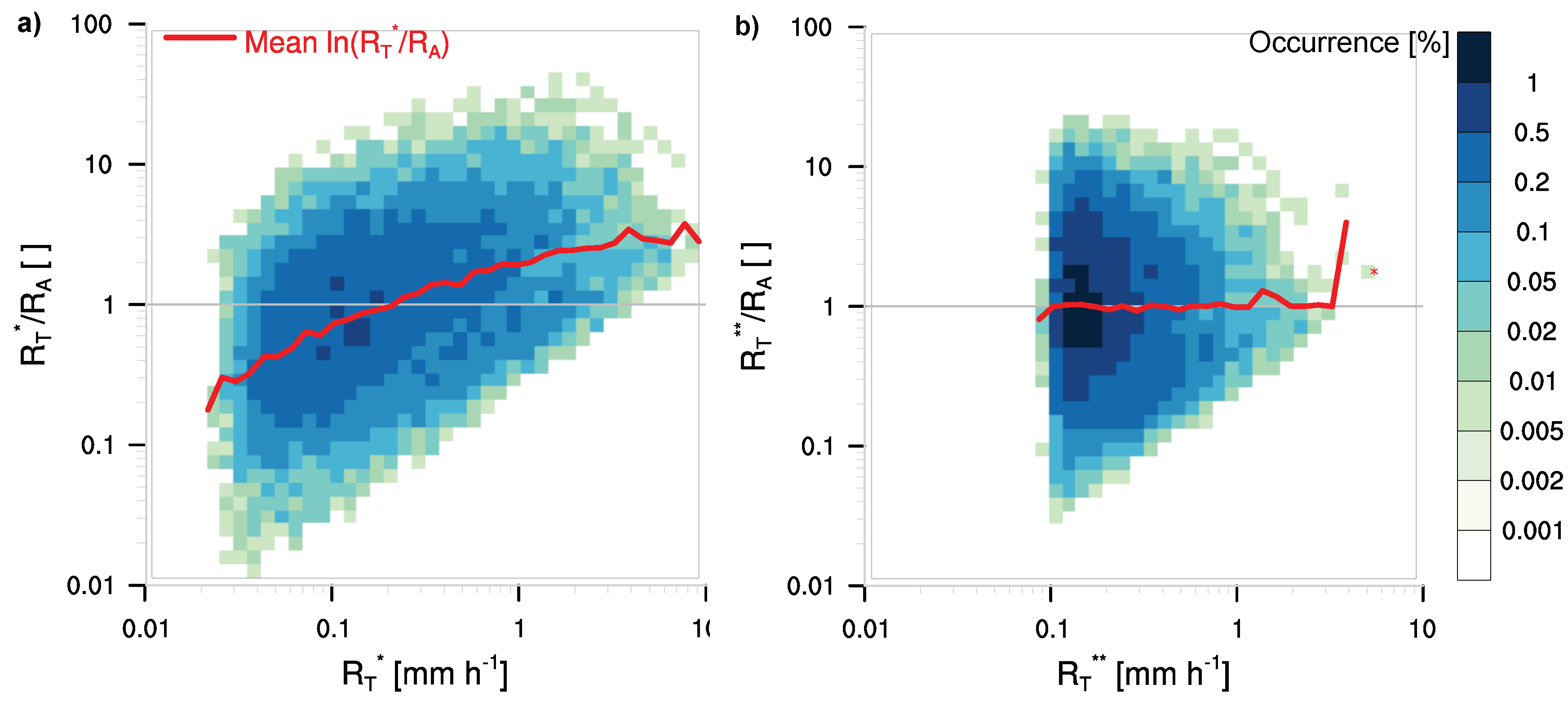
Multiplying each along-track rain rate with the derived adjustment factor of Equation (2) strongly reduces the track–area bias (Figure 4b). However, this statistical adjustment can only serve to reduce an error statistically but not explicitly for individual cases because the spatial rain-rate distribution within the area remains unknown. The resulting -adjusted rain rate , defined as , represents an improved spatial rainfall approximation diagnosed from a track. In the -adjusted along-track rain rate , a bias remains (Figure 5a). This bias represents cases in which the track on average underestimates small rain rates below 0.1 mm h while the track overestimates larger rain rates above 0.5 mm h. This track-to-area deviation in rain rate again follows an exponential fit for with parameters determined by a least squares fit.
The fit reaches for the logarithmically binned mean bias of all 33,265 hit cases with > 2%. Dividing by the median rain rate, , ensures an independence from the used instrument (i.e., S-Pol radar) despite using absolute rain rates. This important step makes the second statistical adjustment usable for different track-like precipitation data sets.
Both statistical adjustments combined strongly reduce the p2a effect in measured precipitation along a ship track compared to a satellite pixel. In order to prove that the statistically adjusted track can better represent rainfall in the area, we calculate the root mean square error (RMSE), given by
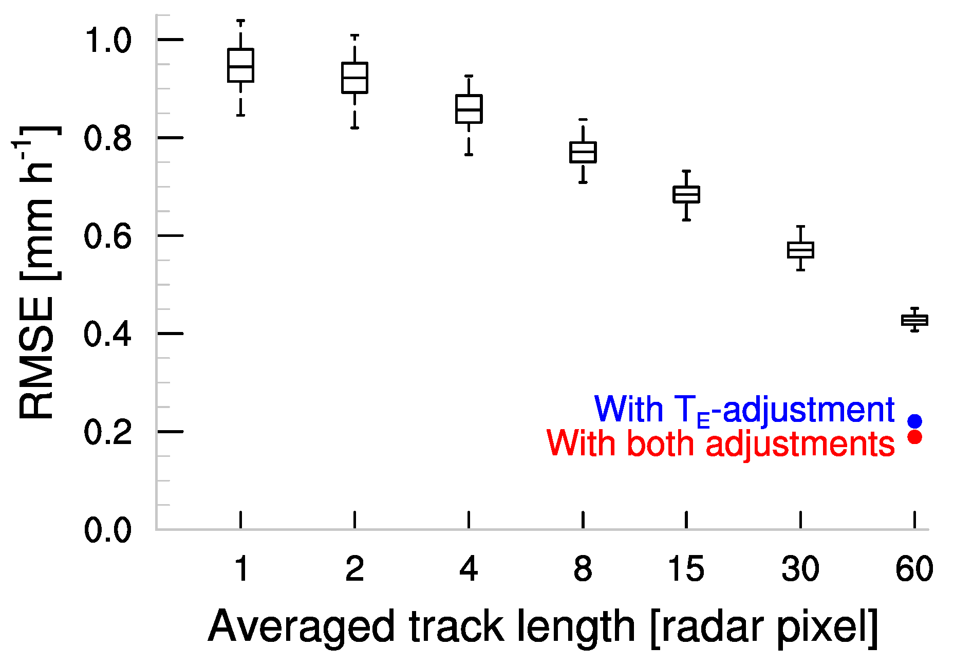
with 234,368 before and after using the adjustments. From an RMSE of initially 0.43 mm h for unadjusted , the -adjustment (Equation (2)) almost halves the RMSE to 0.22 mm h (Figure 6).
Together with the -adjustment (Equation (3)), the RMSE reduces to 0.19 mm h, which corresponds to an overall reduction of 55% with respect to the unadjusted . Overall, both statistical adjustments mark a significant improvement in the representation of along-track rainfall within an area.
Averaging along the simulated track to obtain strongly improves the representation of precipitation in the area. Single point measurements lead to a more than twice as high RMSE of 0.950.04 mm h compared to the longest averaged track length of 60 radar pixels (Figure 6). With increasing averaged track length, the uncertainty obtained from the resampling of 100 realizations of the halved sample size decreases to ±0.01 mm h due to the reduced along-track variability after averaging. Compared to the effect of averaging, the reduction in RMSE after applying the statistical adjustments to corresponds to an averaging track length of more than 100 radar pixels. Both methods represent useful ways to improve the rain-rate representation along a (simulated) ship track.
For the first time, the developed statistical adjustments can address the p2a problem of along-track precipitation measurements on-board ships over the ocean. In contrast to p2a methods for stationary networks of ground-based gauges and radars over land (e.g., [3,28]), shipboard disdrometers produce along-track measurements, which complicates their p2a adjustment. In that respect, the developed statistical adjustments could extend event-based statistics with along-track averaging such as in [14] to reduce the influence of the p2a problem in validating satellite and reanalysis data.
4. Summary and Concluding Remarks
Using island-based radar data, we derived two statistical adjustments for along-track oceanic precipitation data to better represent areal satellite-derived precipitation estimates. Both adjustments statistically correct the tendency of the track to overestimate the rain coverage and to underestimate the rain intensity (both on average). This tendency holds for other ship speeds according to the general statistical relation between track and area, except for very slow-moving ships [29]. The first adjustment uses the average rain event duration along the track, while the second adjustment uses the median-normalized along-track rain rate. Applying these statistical adjustments decreases the RMSE by 0.24 mm h (55%) with respect to the unadjusted along-track averaged rain rate. The averaging along the track also strongly reduces the RMSE compared to using single point measurements or short averaging lengths.
This work represents a step towards a more accurate validation of precipitation derived from PMW satellite sensors using point-like surface precipitation reference data. The derived statistical adjustments are tailored to the spatial resolution of PMW sensor retrieved products such as the HOAPS precipitation parameter with a pixel diameter of about 50 km in the scan resolution product HOAPS-S. The along-track conditions match a typical ship speed in OceanRAIN of about 24–34 km h (depending on track orientation), so that each simulated ship track consists of 60 S-Pol radar pixels. As long as other data sets—both the surface reference data or the satellite data to be validated—do not strongly deviate from these settings, the derived statistical adjustments are generally applicable to other reference data sets for the validation of satellite-derived oceanic precipitation. For differing dataset resolutions, our study might provide guidelines in order to derive individual statistical adjustments to improve the spatial rain-rate representation of along-track reference data.
The statistical adjustments were derived during RICO under typical conditions within the trades. Though these conditions are not globally representative, the statistics of their spatial distribution can cover a wide range of meteorological conditions. Note, however, that snowfall and cold-front precipitation are not represented, while heavy convective rainfall is underrepresented in the statistical adjustments. Their spatial precipitation distribution does not necessarily deviate from the RICO conditions reflected in the adjustments, but the ratio of convective-to-stratiform precipitation can strongly impact the spatial precipitation distribution. Further research using mid- and high-latitude radar data could help to investigate these assumptions.
As they are statistical adjustments, they cannot adjust individual precipitation point measurements or pixels to an area. However, these statistical adjustments are particularly valuable for the validation of satellite-derived data sets that strongly differ in their spatial resolution from that of the reference data set. As usual in statistics, both adjustments reach their maximum utility for large data sets to get the mean precipitation correct while reducing the influence of outliers misrepresenting the areal precipitation rate.
Future studies of oceanic precipitation validation can profit from the derived statistical adjustments to reduce the p2a effect between strongly differing spatial resolutions of satellite data and surface reference data. Thus, we believe that the derived adjustments will not only contribute to a more reliable precipitation estimation over the global ocean, but that they will also add to more accurate validation of other earth observation parameters.
Acknowledgments
The authors thank the crew of RICO for providing the data. This work developed as part of the Ph.D. thesis of J.B. at the Max Planck Institute for Meteorology in Hamburg, Germany in the frame of the research group 1740 funded by the German Research Foundation (DFG). An International Space Science Institute (ISSI) working group on Earth observation validation led by Alexander Löw inspired parts of the analysis. S.A.B. was partially supported by the Cluster of Excellence CliSAP (EXC177), Universität Hamburg, funded through the DFG, by the German Federal Ministry of Education and Research within the framework programme “Research for Sustainable Development (FONA)”, under project HD(CP) (contracts O1LK1502B and O1LK1505D), and by the DFG HALO research program (contract BU2253/3-1). We thank three anonymous reviewers for their helpful comments. Primary data and scripts used in the analysis and other supporting information that may be useful in reproducing this work are archived by the Max Planck Institute for Meteorology and can be obtained by contacting [email protected].
Author Contributions
J.B. designed the experiment, analyzed the data and wrote the manuscript; C.K., S.B. and S.A.B. supported the writing, method development and triggered critical discussions of data analysis results.
Conflicts of Interest
The authors declare no conflict of interest.
References
- Epstein, E.S. Point and area precipitation probabilities. Mon. Weather Rev. 1966, 94, 595–598. [Google Scholar] [CrossRef]
- Ciach, G.J.; Krajewski, W.F. On the estimation of radar rainfall error variance. Adv. Water Resour. 1999, 22, 585–595. [Google Scholar] [CrossRef]
- Porcù, F.; Milani, L.; Petracca, M. On the uncertainties in validating satellite instantaneous rainfall estimates with raingauge operational network. Atmos. Res. 2014, 144, 73–81. [Google Scholar] [CrossRef]
- Michaelides, S.; Levizzani, V.; Anagnostou, E.; Bauer, P.; Kasparis, T.; Lane, J. Precipitation: Measurement, remote sensing, climatology and modeling. Atmos. Res. 2009, 94, 512–533. [Google Scholar] [CrossRef]
- Phillips, D.L.; Dolph, J.; Marks, D. A comparison of geostatistical procedures for spatial analysis of precipitation in mountainous terrain. Agric. For. Meteorol. 1992, 58, 119–141. [Google Scholar] [CrossRef]
- Habib, E.; Ciach, G.J.; Krajewski, W.F. A method for filtering out raingauge representativeness errors from the verification distributions of radar and raingauge rainfall. Adv. Water Resour. 2004, 27, 967–980. [Google Scholar] [CrossRef]
- Stoffelen, A. Toward the true near-surface wind speed: Error modeling and calibration using triple collocation. J. Geophys. Res. Oceans 1998, 103, 7755–7766. [Google Scholar] [CrossRef]
- Alemohammad, S.H.; McColl, K.A.; Konings, A.G.; Entekhabi, D.; Stoffelen, A. Characterization of precipitation product errors across the United States using multiplicative triple collocation. Hydrol. Earth Syst. Sci. 2015, 19, 3489–3503. [Google Scholar] [CrossRef]
- Maggioni, V.; Meyers, P.C.; Robinson, M.D. A Review of Merged High-Resolution Satellite Precipitation Product Accuracy during the Tropical Rainfall Measuring Mission (TRMM) Era. J. Hydrometeor. 2016, 17, 1101–1117. [Google Scholar] [CrossRef]
- Klepp, C. The oceanic shipboard precipitation measurement network for surface validation—OceanRAIN. Atmos. Res. 2015, 163, 74–90. [Google Scholar] [CrossRef]
- Kidd, C.; Huffman, G. Global precipitation measurement: Global precipitation measurement. Meteorol. Appl. 2011, 18, 334–353. [Google Scholar] [CrossRef]
- Tapiador, F.J.; Turk, F.; Petersen, W.; Hou, A.Y.; García-Ortega, E.; Machado, L.A.; Angelis, C.F.; Salio, P.; Kidd, C.; Huffman, G.J.; et al. Global precipitation measurement: Methods, datasets and applications. Atmos. Res. 2012, 104, 70–97. [Google Scholar] [CrossRef]
- Bumke, K. Validation of ERA-Interim Precipitation Estimates over the Baltic Sea. Atmosphere 2016, 7, 82. [Google Scholar] [CrossRef]
- Bumke, K.; König-Langlo, G.; Kinzel, J.; Schröder, M. HOAPS and ERA-Interim precipitation over the sea: Validation against shipboard in situ measurements. Atmos. Meas. Tech. 2016, 9, 2409–2423. [Google Scholar] [CrossRef]
- Keeler, R.; Lutz, J.; Vivekanandan, J. S-Pol: NCAR’s polarimetric Doppler research radar. In Proceedings of the 2000 International Geoscience and Remote Sensing Symposium (IGARSS 2000), Honolulu, HI, USA, 24–28 July 2000; Volume 4, pp. 1570–1573. [Google Scholar]
- Rauber, R.M.; Ochs, H.T.; Di Girolamo, L.; Göke, S.; Snodgrass, E.; Stevens, B.; Knight, C.; Jensen, J.B.; Lenschow, D.H.; Rilling, R.A.; et al. Rain in Shallow Cumulus Over the Ocean: The RICO Campaign. Bull. Am. Meteorol. Soc. 2007, 88, 1912–1928. [Google Scholar] [CrossRef]
- Burdanowitz, J.; Nuijens, L.; Stevens, B.; Klepp, C. Evaluating light rain from satellite- and ground-based remote sensing data over the subtropical North Atlantic. J. Appl. Meteorol. Climatol. 2015, 54, 556–572. [Google Scholar] [CrossRef]
- Behrangi, A.; Lebsock, M.; Wong, S.; Lambrigtsen, B. On the quantification of oceanic rainfall using spaceborne sensors. J. Geophys. Res. 2012, 117, 105. [Google Scholar] [CrossRef]
- UCAR/NCAR-Earth Observing Laboratory. S-PolKa: S-band/Ka-band Dual Polarization, Dual Wavelength Doppler Radar. 1996. Available online: https://doi.org/10.5065/D6RV0KR8 (accessed on 29 September 2016).
- Knight, C.A.; Miller, L.J. Early Radar Echoes from Small, Warm Cumulus: Bragg and Hydrometeor Scattering. J. Atmos. Sci. 1998, 55, 2974–2992. [Google Scholar] [CrossRef]
- Snodgrass, E.R.; Di Girolamo, L.; Rauber, R.M. Precipitation Characteristics of Trade Wind Clouds during RICO Derived from Radar, Satellite, and Aircraft Measurements. J. Appl. Meteorol. Climatol. 2009, 48, 464–483. [Google Scholar] [CrossRef]
- UCAR/NCAR-EOL. RICO: S-band Polarimetric (S-Pol) Data DORADE Format. Version 1.0. 2011. Available online: https://data.eol.ucar.edu/dataset/87.008 (accessed on 29 September 2016).
- Max Planck Institute for Meteorology. Climate Data Operators. 2015. Available online: http://www.mpimet.mpg.de/cdo (accessed on 16 May 2017).
- Brueck, M.; Nuijens, L.; Stevens, B. On the Seasonal and Synoptic Time-Scale Variability of the North Atlantic Trade Wind Region and Its Low-Level Clouds. J. Atmos. Sci. 2015, 72, 1428–1446. [Google Scholar] [CrossRef]
- Nuijens, L.; Stevens, B.; Siebesma, A.P. The Environment of Precipitating Shallow Cumulus Convection. J. Atmos. Sci. 2009, 66, 1962–1979. [Google Scholar] [CrossRef]
- Andersson, A.; Fennig, K.; Klepp, C.; Bakan, S.; Graßl, H.; Schulz, J. The Hamburg Ocean Atmosphere Parameters and Fluxes from Satellite Data—HOAPS-3. Earth Syst. Sci. Data 2010, 2, 215–234. [Google Scholar] [CrossRef]
- Fennig, K.; Andersson, A.; Bakan, S.; Klepp, C.P.; Schröder, M. Hamburg Ocean Atmosphere Parameters and Fluxes from Satellite Data—HOAPS 3.2—Monthly Means/6-Hourly Composites. Satell. Appl. Facil. Clim. Monit. (CM SAF) 2012. [Google Scholar] [CrossRef]
- Wagner, P.D.; Fiener, P.; Wilken, F.; Kumar, S.; Schneider, K. Comparison and evaluation of spatial interpolation schemes for daily rainfall in data scarce regions. J. Hydrol. 2012, 464–465, 388–400. [Google Scholar] [CrossRef]
- Burdanowitz, J. Point-to-Area Validation of Passive Microwave Satellite Precipitation with Shipboard Disdrometers. Ph.D. Thesis, Universität Hamburg, Hamburg, Germany, 2017. [Google Scholar]
Figure 1.
Photo (a) shows S-Band Polarimetric (S-Pol) radar during RICO (Rain In Cumulus clouds over the Ocean; Copyright University Corporation for Atmospheric Research (UCAR) by Gordon Farguharson, licensed under CC BY-NC 4.0 License via OpenSky). Example of S-Pol radar image interpolated on Cartesian grid (b) with red boxes that are chosen to simulate the satellite pixels. Enlarged red box (c) illustrates 16 randomly chosen synthetic ship tracks (blue dotted lines; 5 horizontal, 5 vertical, 6 diagonal) of 60 radar pixels, each corresponding to a typical ship speed of 24–34 km h depending on track orientation. For clarity, the number of sketched radar pixels is only one tenth of the original grid (Section 2.2). PMW: passive microwave.

Figure 2.
The frequency of occurrence (%) of hits ( > 0 and > 0; blue solid line), misses ( = 0 and > 0; red dotted line), and zero rain cases ( = 0 and = 0; gray dashed line) for the S-Pol data as a function of the minimum area rain coverage (%). The sum of hits, misses, and zero rain always adds up to 100%, as in Table 1.
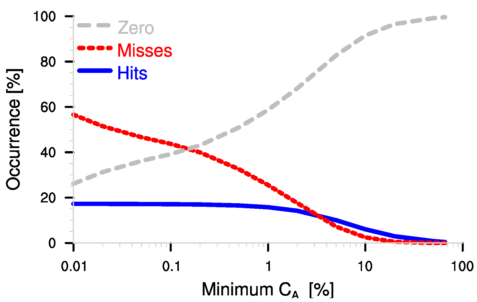
Figure 3.
(a) 2D histogram with relative occurrence in % of all 40,538 hit cases shown as colors of average rain-rate ratio as a function of the rain coverage ratio ; and (b) the conditional rain-rate ratio . Solid gray 1-by-1 line marks maximum possible dependence of on either or , while the other ratio needs to be 1 (gray dotted lines) because of .

Figure 4.
(a) 2D-histogram with relative occurrence (%) shown as colors of the rain-rate ratio as a function of the along-track average rain event duration for uncorrected ; and (b) corrected for > 2% using Equation (2). Red lines mark the mean of and per bin, gray lines highlight for which equals or , respectively.

Figure 5.
(a) 2D-histogram with relative occurrence (%) of the -adjusted average rain-rate ratio ; and (b) the - and -adjusted average rain-rate ratio both as a function of and , respectively. Red line marks logarithmic mean per bin.
Figure 5.
(a) 2D-histogram with relative occurrence (%) of the -adjusted average rain-rate ratio ; and (b) the - and -adjusted average rain-rate ratio both as a function of and , respectively. Red line marks logarithmic mean per bin.

Figure 6.
RMSE (mm h) shown as a function of averaging length in radar pixel units. Black boxes (interquartile spread, median) and whiskers (minimum, maximum) mark uncertainty obtained from resampling of 100 realizations of unadjusted , while the blue dot marks the RMSE of , and the red dot of , respectively.

Table 1.
Contingency table lists relative occurrence (%) of rain-rate combinations for (along-track rain rate) and (area rain rate) from 234,368 available cases. In contrast to the left part of the table, the right part sets if %. Note that tracks are always located completely within the area such that can only occur if (no false detections possible).
| All Cases | % | |||
|---|---|---|---|---|
| 17.3 | 61.2 | 14.2 | 17.6 | |
| 0 | 21.5 | 0 | 68.2 | |
© 2017 by the authors. Licensee MDPI, Basel, Switzerland. This article is an open access article distributed under the terms and conditions of the Creative Commons Attribution (CC BY) license (http://creativecommons.org/licenses/by/4.0/).
Share and Cite
MDPI and ACS Style
Burdanowitz, J.; Klepp, C.; Bakan, S.; Buehler, S.A. Simulation of Ship-Track versus Satellite-Sensor Differences in Oceanic Precipitation Using an Island-Based Radar. Remote Sens. 2017, 9, 593. https://doi.org/10.3390/rs9060593
AMA Style
Burdanowitz J, Klepp C, Bakan S, Buehler SA. Simulation of Ship-Track versus Satellite-Sensor Differences in Oceanic Precipitation Using an Island-Based Radar. Remote Sensing. 2017; 9(6):593. https://doi.org/10.3390/rs9060593
Chicago/Turabian StyleBurdanowitz, Jörg, Christian Klepp, Stephan Bakan, and Stefan A. Buehler. 2017. "Simulation of Ship-Track versus Satellite-Sensor Differences in Oceanic Precipitation Using an Island-Based Radar" Remote Sensing 9, no. 6: 593. https://doi.org/10.3390/rs9060593
Note that from the first issue of 2016, this journal uses article numbers instead of page numbers. See further details here.