Supervised Classification of Power Lines from Airborne LiDAR Data in Urban Areas


1
National-Local Joint Engineering Laboratory of Geo-Spatial Information Technology, Hunan University of Science and Technology, No. 1 Taoyuan Road, Xiangtan 411201, China
2
Department of Geography, University of Hawaii at Mānoa, 2424 Maile Way, Honolulu, HI 96822, USA
3
Department of Geography, University of Cincinnati, Braunstein Hall, 400E, Cincinnati, OH 45221, USA
4
School of Geography and Planning, Sun Yat-Sen University, 135 Xingangxi Road, Guangzhou 510275, China
*
Authors to whom correspondence should be addressed.
Remote Sens. 2017, 9(8), 771; https://doi.org/10.3390/rs9080771
Submission received: 10 May 2017
/
Revised: 12 July 2017
/
Accepted: 21 July 2017
/
Published: 28 July 2017
Abstract
:Automatic extraction of power lines using airborne LiDAR (Light Detection and Ranging) data has been one of the most important topics for electric power management. However, this is very challenging over complex urban areas, where power lines are in close proximity to buildings and trees. In this paper, we presented a new, semi-automated and versatile framework that consists of four steps: (i) power line candidate point filtering, (ii) local neighborhood selection, (iii) spatial structural feature extraction, and (iv) SVM classification. We introduced the power line corridor direction for candidate point filtering and multi-scale slant cylindrical neighborhood for spatial structural features extraction. In a detailed evaluation involving seven scales and four types for local neighborhood selection, 26 structural features, and two datasets, we demonstrated that the use of multi-scale slant cylindrical neighborhood for individual 3D points significantly improved the power line classification. The experiments indicated that precision, recall and quality rate of power line classification is more than 98%, 98% and 97%, respectively. Additionally, we showed that our approach can reduce the whole processing time while achieving high accuracy.

1. Introduction
Inspection of power lines to detect and eliminate hidden risks is an important task for urban and rural power supply management and scientific planning [1,2]. However, power lines stretch across long geographical distances, making it labor-intensive and costly to conduct traditional field-based inspection. In contrast, airborne LiDAR (light detection and ranging) can directly collect high-precision 3D point cloud data of the power line corridor, saving a lot of field survey time and labor [3,4]. Nevertheless, airborne LiDAR data volume is large and power lines are usually close to vegetation and buildings over urban areas. These make it difficult to extract urban power line points accurately and quickly from LiDAR point cloud. Therefore, the development of highly efficient, rapid and automated methods for extracting urban power lines from airborne LiDAR point cloud data is a critical issue.
The conventional methods for power line extraction include: (i) statistical analysis of point clouds based on height, density or number of pulses, etc. [5,6,7]; (ii) Hough transform and clustering based on 2D image processing [5,8,9,10,11]; (iii) supervised classification based on geometrical and distribution features of laser points [2,12,13,14].
To filter power line points from raw LiDAR data, Zhu and Hyyppa [5,15] conducted statistical analysis based on criteria involving metrics such as height and density and 2D image-based processing that considers geometric properties. These methods were designed for forest areas and the average accuracy was 93.26%. However, in complex urban scenes where trees and buildings are close to power lines (mainly distribution lines), the classification accuracy could decrease. Clode and Rottensteiner [16] introduced a tree and power line classification method based on the theory of Dempster-Shafer for data fusion, for which the accuracy of classification was only 64%. Guan et al. [6] extracted power lines from mobile vehicle-based LiDAR data using filters based on height, spatial density and a combination of size and shape, while Cheng et al. [7] extracted urban power lines using a voxel-based hierarchical method and a bottom-up filtering method. The accuracy of power line classification in [6,7] was 92–93.9%. However, such high accuracies can be partially attributed to the high point density of mobile LiDAR data. It is expected that lower accuracies will be obtained if airborne LiDAR data of lower point density are used.
Power lines can be detected from the horizontal XOY plane using image processing techniques; in such cases, Hough transform and Radon transform have often been used [8,9,11]. Sohn et al. [10] used the voting scheme to extract linear candidate points and then converted into line segments by 3D line fitting based on RANdom SAmple Consensus (RANSAC) [17], the overall accuracy of power line classification was 91.3%. Melzer and Briese [18] used Hough transform to detect 2D segmented power line primitives; the reconstruction of power lines was accomplished by using the random sampling consistency algorithm to select the power line primitives for estimating the vertical parameters.
For supervised classification of power lines, Kim and Sohn [12] and Guo et al. [13] extracted 21 features to characterize the horizontal and vertical properties of power line objects and used knowledge-based classification methods to separate power lines from their background in two steps by fitting in the XOZ or YOZ plane. These methods needed to use contextual pylon information and the accuracy of point-based classification was 91.04% and 89%, respectively. References [19,20,21] extracted power lines and towers according to the semantic relationship based on the position of towers. The methods were unsuitable for power line classification in complex urban scenes where small electric poles instead of tall towers are ubiquitous. Liang et al. [22] used the fact that the same power line is closely linked to extract power lines from the point cloud, but the method requires airborne LiDAR point cloud of very high density. Ritter and Benger [23] proposed to detect power line candidate points by using the non-linear adjustment of the catenary line, but the method is computationally complex and had large omission errors.
Machine learning is a powerful supervised statistical method that can be used to classify power line points from 3D LiDAR data. The popular classifiers for laser point classification include Support Vector Machine (SVM) [24,25], Random Forests [12,26], JointBoost [19] and so on. The feature extraction for supervised classifiers is a crucial issue. Point-level features are commonly used to construct the feature vectors [14,19,25,27,28,29]. Furthermore, many studies [14,26,30,31] extracted interpretable geometrical and distributional features from the local neighborhood of each laser point, for which the determination of local neighborhood type and size is a critical issue. Previous studies typically used vertical cylindrical or spherical neighborhoods [26,32,33] for classifying ground, buildings and trees, but rarely for power lines. It is relatively unknown how such methods work for power line extraction.
Overall, despite of many previous studies, the classification and extraction of power line points from airborne LiDAR data over urban areas remain a challenge: the accuracy is usually not very high due to the close proximity of power lines with buildings and vegetation; moreover, fast algorithms are needed to process large volume of LiDAR data [34,35]. In this study, we proposed an accurate and fast power line classification method that works over complex urban scenes. The method is based on supervised classification and thus requires useful features that can effectively distinguish power lines. Our method is novel in that (i) it derives features from local neighborhood that is designed specifically for power line extraction, and (ii) it has superior performance in data processing time.
2. Materials and Methods
We designed our novel methodology for power line point cloud classification based on geometric multi-scale features and multi-scale neighborhood types. The main components of this methodology consist of (i) power line candidate point filtering, (ii) local neighborhood selection, (iii) spatial structural feature extraction and (iv) SVM classification, which are explained in Figure 1 and the following subsections.
2.1. Dataset
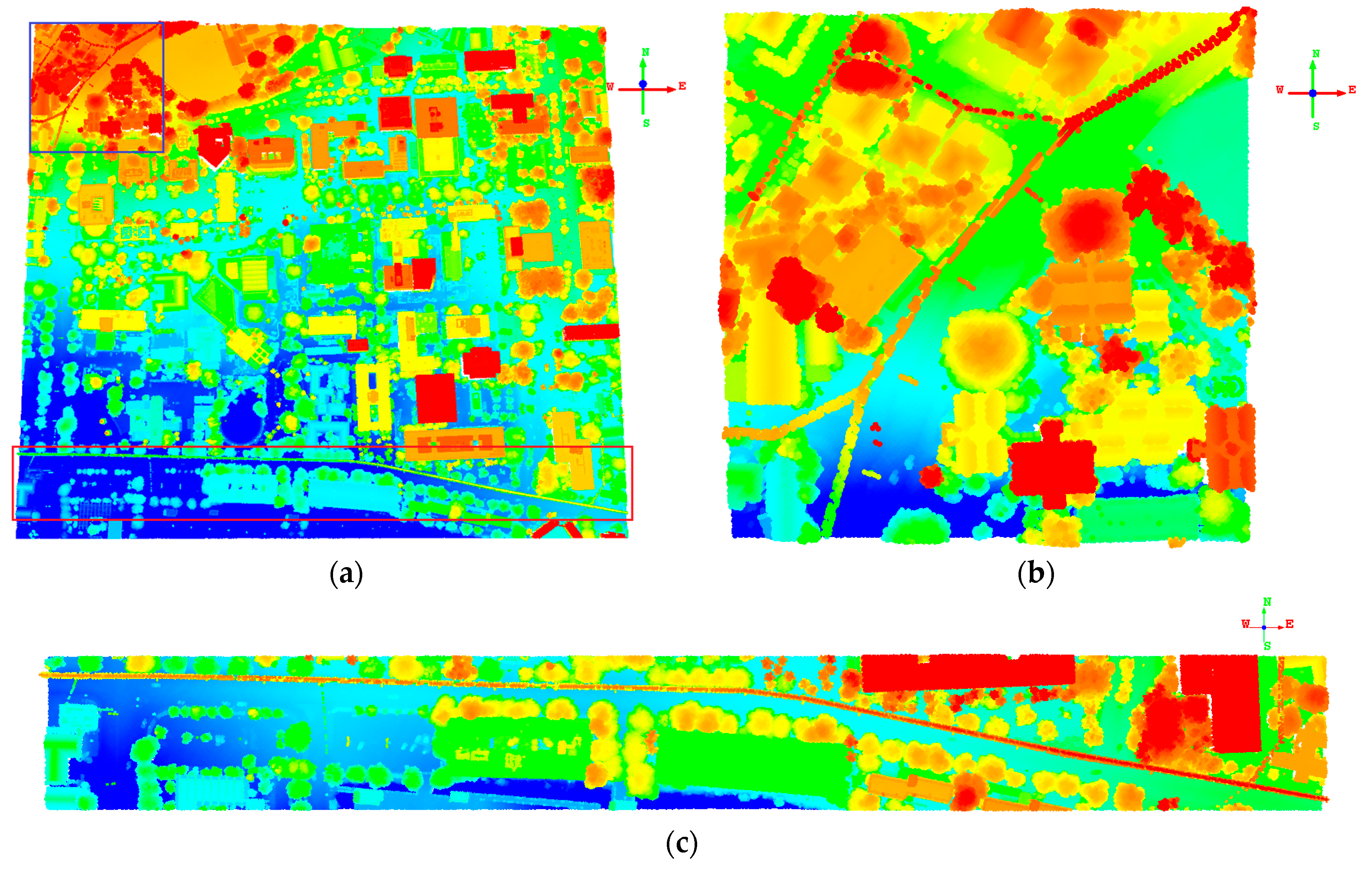
Our study site is an urban area surrounding the campus of University of Hawaii at Manoa in Honolulu, Hawaii. The airborne LiDAR data were acquired in summer 2013 using Optech ALTM GEMINI laser system (scan rate: 37 Hz; laser pulse rate: 70,000 Hz; multi-pulse in air mode enabled with up to five echoes) mounted on a twin-engine Piper PA-31 Navajo airplane (aboveground flight height: ~800–1400 m). The datasets for our research consist of upper left area (which is referred to as UL Dataset, 180 × 180 m2) and lower part area (which is referred to as LP Dataset, 800 × 100 m2) from a large LiDAR scene that covers the study site (Figure 2). The power lines in these datasets are urban distribution lines. The point density is ~3.4 points/m2. For both UL Dataset and LP Dataset, ground truth is available in the form of a manual point-wise labelling of the power line class. An overview of the number of labelled 3D points for power lines is given in Table 1.
2.2. Power Line Candidate Filtering
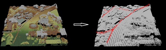
The power line candidate point filtering from raw LiDAR point cloud is the first step for power line classification. This step was to reduce the volume of processed airborne-based LiDAR points while retaining all possible power line points. We proposed a refined method of filtering power line from the original LiDAR point cloud with two sub-steps: (i) ground points and non-ground points separation (Section 2.2.1), (ii) power line corridor direction construction (Section 2.2.2), which was to find the corridor lines and extract the power line candidate points based on the corridor direction.
2.2.1. Ground Points and Non-Ground Points Filtering
The ground point classification is a key step for generating DTM (Digital Terrain Model) from airborne LiDAR point cloud. Researchers have developed a wide range of LiDAR data ground filtering algorithms, including segmentation- and cluster-based filters, morphological filters, directional scanning filters, contour-based filters, etc. [36,37,38,39]. In this paper, we first applied the Tiffs (Toolbox for LiDAR Data Filtering and Forest Studies) software [34] and its edge-based morphological method [40] for conducting ground points classification and DTM generation and then selected all points that are 4 m above ground [5] as power line candidate points.
2.2.2. Power Line Corridor Direction Construction
The points above ground or terrain in LiDAR point cloud may contain non-powerline objects such as building and trees, which need to be separated from power lines. Power lines have unique geographical characteristics as follows: distributed regularly between two neighboring electric towers or poles with sag and other physical properties [2,6,13,41]. This knowledge can be used to screen power lines in large LiDAR data scene.
We proposed a power line corridor direction construction algorithm based on Hough transform [8,9] and RANdom SAmple Consensus (RANSAC) rule [17]. The specific procedure is as follows.
Step 1: Extract lines from the filtered LiDAR points. The power line points have a linear distribution on the O-XY plane. We used the Hough transform to obtain the linear objects from the non-ground LiDAR points. First, the point cloud data were converted to 2D raster image of O-XY plane, which contains the parameters such as raster cell size for segmentation, the resolution of intercept and angle, etc. The conversion from point coordinate to polar coordinate parameter space was computed by the equation:
where represents the intercept and represents the slope angle of the points in one line. So, a pair of parameters can represent the line.
After that, we can extract the peak value to obtain the possible lines from the projected parameter space , which is also called Hough transform matrix. According to the resolution of and , the accumulated peak number of same and may be from points in one line. We can extract different lines by the threshold parameters of line distance (15 m), line width (5 m), and peak number (, where is the maximum value of the Hough transform matrix H). These threshold parameters are related to the minimum linear distance and width of power lines. We adjusted these parameters to make sure the extract lines will not miss potential power lines.
Step 2: Extract possible power lines. The lines extracted by Hough transform may be very piecemeal, redundant and contain outliers. Each probable line has four parameters: the project parameters and , the origin point and destination point , which are . We used the RANSAC algorithm to extract the line candidates. The power line candidates are continual and not strictly linear. The points of power line are denser than other places. The formula of line candidates is as follows:
Step 3: Extract the power line candidate points. Create small buffers for these possible power lines. The width of the buffers is about two times of the width of power line corridor. Denote the points in the buffers as the power line candidate points.
The power line candidate filtering we proposed in this study differs from the methods in [5,7,13], which mainly used laser point height, density or other parameters to separate the power line candidate points from raw LiDAR point cloud. Here, we not only used point height or density but also incorporated information about the power line corridor direction. As shown in Figure 3, the power line candidate filtering reduced the data volume and retained the possible power line points for further processing.
2.3. Local Neighborhood Selection
2.3.1. Neighborhood Type Determination
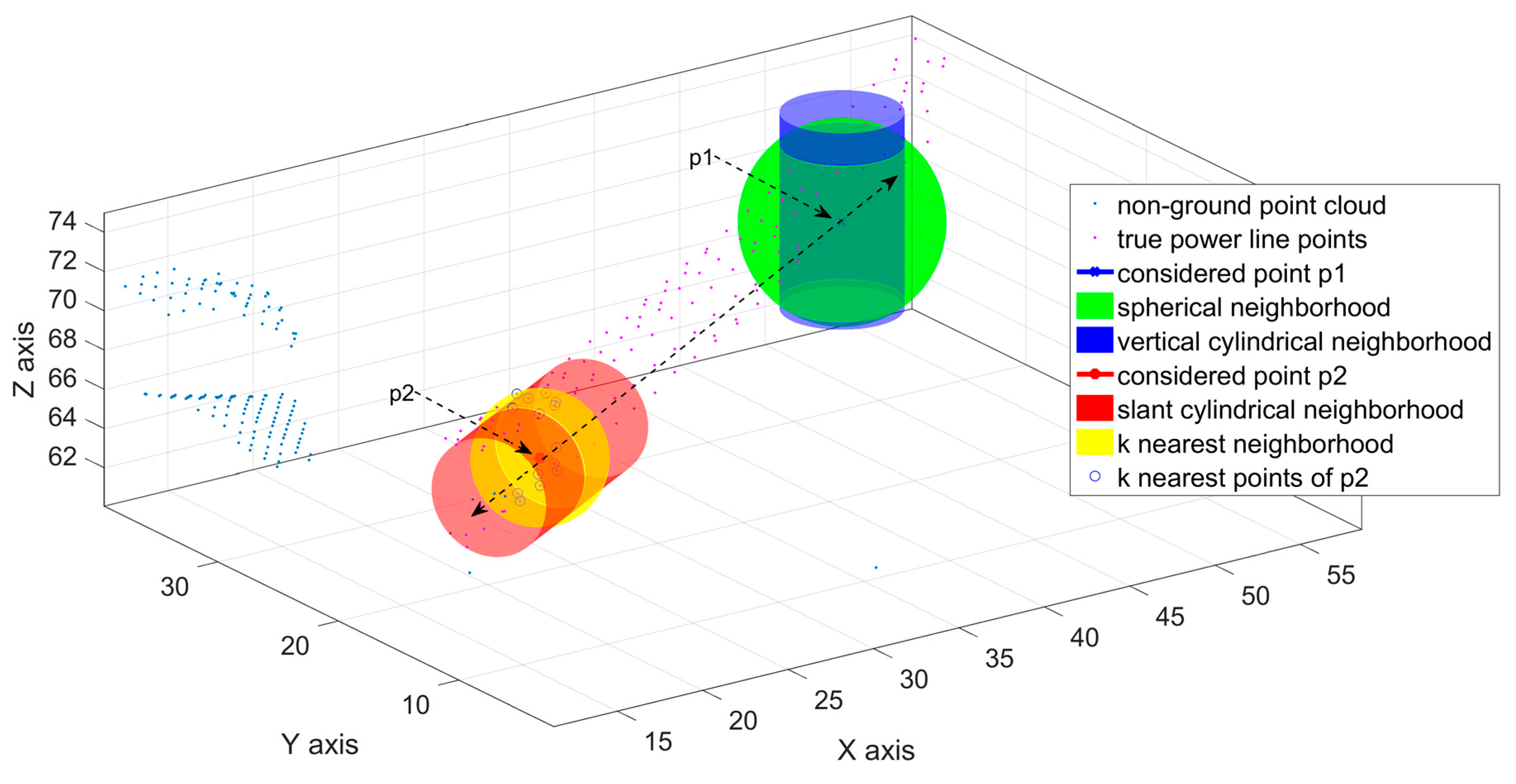
We considered four commonly used neighborhood types: spherical, vertical cylindrical, k nearest, and slant cylindrical neighborhoods, which are defined using different geometrical parameters as follow:
- a spherical neighborhood is formed by all 3D points within a sphere around point P, which is parameterized with a fixed radius,
- a vertical cylindrical neighborhood is formed by all 3D points within a vertical cylindrical whose axis vertically passes through point P and whose radius is fixed,
- a k nearest neighborhood is formed by the nearest neighbors of considered point P, the k is its parameter, and
- a slant cylindrical neighborhood is formed by all 3D points with a slant cylindrical whose radius is fixed and whose axis passes through considered point P along with the direction of power line corridor.
2.3.2. Neighborhood Scale Selection
We characterized the local 3D structure of point P using neighborhoods of both single-scale and multi-scale. The single-scale neighborhood corresponds to each local neighborhood type defined with a fixed parameter. The parameters for each single-scale neighborhood, as explained in the previous section, include radius or nearest k number, optimal neighborhood for individual 3D points based on eigenvalues [31]. However, it is difficult to choose a fixed parameter that can optimally work for power line corridors of different complexities.
The multi-scale neighborhood was chosen to address the above problem by combining structure information from multiple scales. This corresponds to the use of different radii for cylindrical neighborhoods or different k values for k nearest neighborhood. The choice of different radii and k was based on previous studies [14,26,31,32] and adjusted for our study. See Figure 4 for a comparison of the four different neighborhood types.
2.4. Spatial Structural Feature Extraction
The successful identification of power line points depends on the extractions of useful features that can distinguish power lines from other objects. To characterize local neighborhood 3D points based on their coordinates, geometric and distribution features have been proposed and used in many studies [25,26,31,32,42]. The geometrical features focused on the fit parameters of geometric primitives (e.g., planes, spheres or cylinders) and evaluated certain geometric measures, while distribution features focused on describing the local context by sampling a distribution. As summarized as above, such metrics have rarely been used in power line classification. For a point P and its local neighborhood points set , we followed [26,31,32] and used 3D features based on eigenvalues and corresponding normalized eigenvalues of the covariance tensor and is its central point. We applied the method in [26] to extract 26 features set (see Table 2 for a partial list).
2.5. SVM Classification
We used SVM [24] for classifying power line points. The extracted features based on the local individual points’ neighborhood are the predictors for the SVM classifier. To calibrate and validate SVM, we manually identified true power line points from our dataset and used five-fold cross-validation to assess the classifier’s accuracy.
SVM is a popular mathematical tool, which is based on risk minimization principle, and it tries to find a high dimensional feature space to solve some inseparable classification problems. The kernel function is introduced into SVM so that the original input feature space can be transformed into a higher dimensional space. We tried different kernel functions and found that the Gaussian radial basis function (RBF) was effective in this study:
where represents the RBF kernel parameter and was tuned iteratively to adjust the better classification results.
2.6. Experiments
The neighborhood used for extracting structural features plays a crucial role for the classification of power line points. Therefore, following the procedure described in Section 2.2, Section 2.3, Section 2.4 and Section 2.5, we did a comparative analysis of power line classification using two different neighborhood scales (single-scale and multi-scale) and four neighborhood types (spherical, vertical cylindrical, k nearest and slant cylindrical neighborhoods).
Specifically, we did two kinds of comparative experiments: (i) neighborhood scale experiments based on spherical neighborhood, involving six spherical single-scale neighborhoods denoted as , , , , and , one spherical multi-scale neighborhood denoted as resulting from the combination of neighborhoods , , , , and . We chose spherical neighborhood with 1 m, 3 m, or 5 m as its radii because it was commonly used in previous studies [14,26,31,32]. In order to evaluate the effect of different scales and multi-scale, we added 7 m, 9 m and 11 m as the radii; (ii) neighborhood types experiment based on multi-scale neighborhood, involving spherical, vertical cylindrical, k nearest and slant cylindrical neighborhoods, denoted correspondingly as , , and . The structural feature sets for each local neighborhood scale and type were computed by the method in Section 2.4 and concatenated to a feature vector as inputs for the SVM classifier.
In order to compare the classification results obtained with the different approaches at point-level, we consider a variety of measures for evaluation on the power line classification: (i) precision rate (), (ii) recall rate (), (iii) quality rate () and (iv) processing time (). The contains the whole processing time from power line candidate filtering to SVM classification. The , and are computed as follows:
where is the sum of true positives for power lines, is the sum of false positives for power lines, is the sum of false negatives for power lines, depicts the percentage of in the power lines classification results, depicts the percentage of in the reference data, depicts the quality percentage as an overall measurement. The algorithm proposed was programmed in Matlab (the Mathworks, Inc., Natick, MA, USA). The computer we used has 8 GB RAM and a dual-core 2.20 GHz processor.
3. Results
3.1. Single-Scale and Multi-Scale Neighborhoods
Table 3 summarizes the results of using spherical neighborhoods at six single scales and one multi-scale for two datasets. It showed that had the best performance among the six single scale neighborhoods in UL dataset, while had the best performance in LP dataset. The optimal scale (7 m) of the UL dataset is smaller than the optimal scale (9 m) of the LP dataset. This is because that power lines of UL dataset are closer to trees and buildings. The scale of the highest accuracy could also be related to the width of power line corridor, which is about 5 m in UL dataset and about 7 m in the LP dataset. For processing time , took longer than other single-scale ones, mainly because of the longer time for the classification step. This indicates that at the local scale () it is more difficult to separate power lines from other objects.
The multi-scale neighborhood had higher , and than the six single scale neighborhoods because it incorporates more information than any single-scale neighborhood. The cost, however, is that it took longer to extract features in multi-scale neighborhoods. Even so, we think it is overall advantageous to use multi-scale neighborhoods because the best single-scale neighborhood varies from site to site and is unknown a priori. Therefore, we chose multi-scale neighborhood for the next experiments.
3.2. Different Neighborhood Types
Table 4 compared the classification results in the four different neighborhood types (, , , ). , and neighborhoods were based on the multi-scale local neighborhood, while was based on optimal nearest k and eigenvalues [26,31].
The results in Table 4 showed that the neighborhood type of has the best result in these experiments. The result of neighborhood is the same as multi-scale neighborhood in Section 3.1 The , and in and are similar while the neighborhood type has lowest values. The k number in is iteratively computed for each point, so the processing time is much higher in LP dataset. For , the computation time is substantially less due to the use of the power line corridor direction to reduce the power line candidate points.
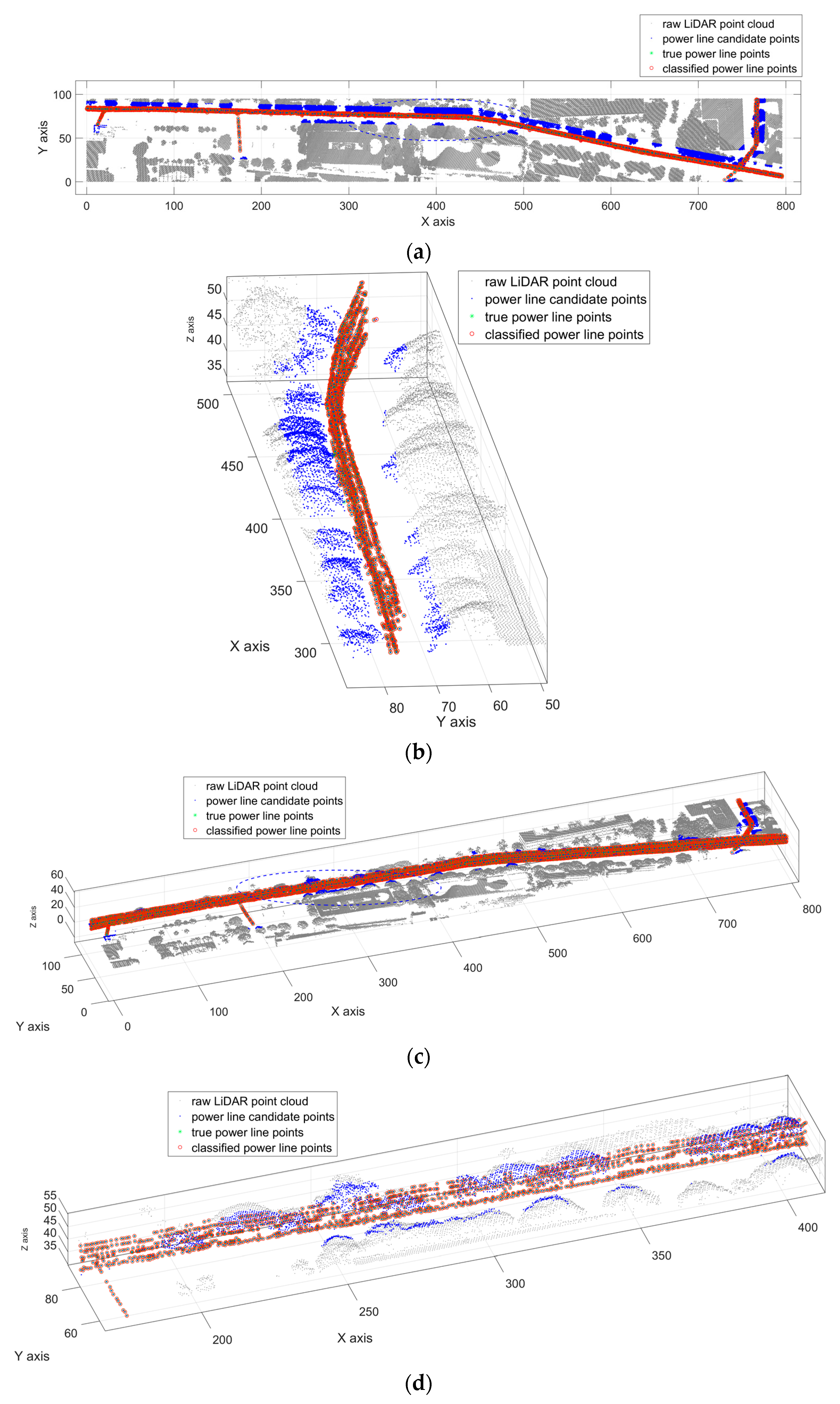
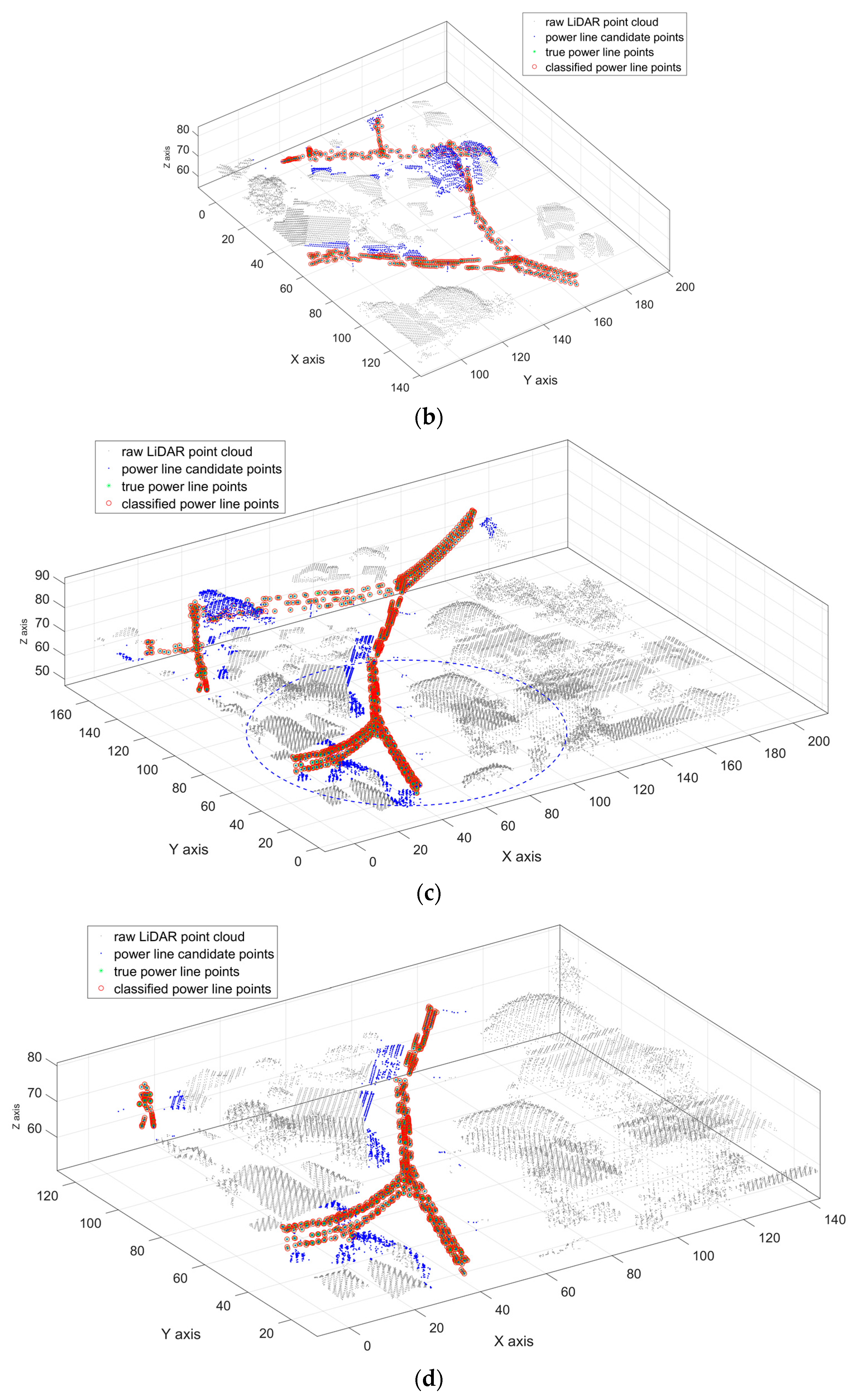
Exemplary classification results of multi-scale slant cylindrical neighborhood are shown in Figure 5 and Figure 6. In these figures, the gray points represent the raw LiDAR point cloud, the blue points represent the power line candidate points filtered by corridor direction, the green points (marked by ‘*’) represent the true power line points, and the red points (marked by ‘o’) represent the power line classification result.
4. Discussion
The novelty of this study is to use multi-scale slant cylindrical neighborhood and to introduce power line corridor direction to characterize the spatial structure of power lines for classification. Different from previous studies [5,13,14,19,26,31,32], which first rasterized LiDAR points and then used image-based processing technology for power line extraction or extracted features based on optimal k and eigenvalues, our approach focused on spatial structural characterisation of 3D points via feature extraction from different scales and types of local neighborhoods and performed point-wise classification. Our datasets are from an urban area where power lines are in close proximity to vegetation or building. The point density (3.4 point/m2) of our LiDAR data is relatively low relative to the ones reported in published research, for which some can reach up to 150 points/m2 [7]. Despite of these challenges, our method can still achieve high classification accuracy.
4.1. Influence of Power Line Corridor Direction
The power line corridor direction is used in candidate filtering and local neighborhood selection to decrease the data volume of processing LiDAR points and improve the accuracy of classification results. Comparing with other studies [5,7,16], the parameters (density, echo number, intensity, etc.) were not used for power line candidate filtering from raw airborne LiDAR point cloud. The density in airborne LiDAR data is not as high as vehicle-based mobile LiDAR data [7] and the density of upper power lines is higher than the lower’s. While in the urban area, the complex environment that power line points mixed with building or trees makes the height and density of different objects are similar. So, these filtering methods in [5,16] may be not suitable for power line candidate filtering.
By considering the power line corridor direction, the PREC, REC and QUA of classification results of slant cylindrical neighborhood were improved by up to 2.8% compared with other commonly used neighborhoods, such as , , [14,26,31,32]. Compared with the neighborhood of optimal size [31], the whole processing time was reduced from 152 s to 18 s in UL dataset and from 1513 s to 98 s in LP dataset.
The power line corridor direction was extracted by Hough transform and RANSAC algorithm, which requires threshold values of line length, line width, resolution of angle and intercept and so on. This is an extra burden for a user. However, if the information about power line corridor direction is available in advance (i.e., via field survey, historical archives), it can be easily incorporated into our algorithm, even if such information is only approximate.
4.2. Benefit of Power Line Neighborhood Selection
Among the four types of neighborhood (spherical, cylindrical, k nearest and slant cylindrical neighborhood), we found that the spherical, cylindrical and k nearest neighborhood based on the radius and optimal eigenvalues did not perform as well as the slant cylindrical neighborhood. This is because the structural feature sets based on the slant cylindrical neighborhood are from the approximate power line corridor direction and thus are less affected by other objects such as buildings and trees.
In our experiments, the power lines are ~4 m above the ground with ~2 m spacing and 5–7 m total width. We found that the better radius of single-scale neighborhoods is 7 m and 9 m in UL dataset and LP dataset, respectively.
These optimal scales approximate the horizontal or vertical span of the power lines. Multi-scale neighborhoods performed better because of the spatial heterogeneity of the environment. The multi-scale slant cylindrical neighborhood is based on the multiple radii and power line corridor direction. This type of neighborhood is tailored to power line characteristics and thus had the best performance.
5. Conclusions
In this study, we proposed a novel methodology for classifying power line from airborne laser scanning data. The method consists of power line candidate filtering, local neighborhood selection, geospatial structural feature extraction, and SVM classification. We extracted the power line corridor direction by Hough transform and RANSAC algorithm. The corridor direction was used to construct a multi-scale cylindrical neighborhood for power line classification. We evaluated this method for seven neighborhood scales and four neighborhood types over complex urban areas. We found that feature extraction based on the multi-scale slant cylindrical neighborhood led to improved classification results in comparison to single-scale neighborhood and other neighborhood types. In future work, we plan to test the methodology for different types of points cloud data (e.g., mobile laser scanning data) or to use the classification results for 3D reconstruction of power lines in complex urban environments. Although the accuracy of power line classification is high for our dataset and study area, we need more research in the future to test the generality of our method over different sites using airborne LiDAR data collected by different settings.
Acknowledgments
This work is supported by the National Natural Science Foundation of China (Grants 41601426). The authors thank the anonymous reviewers and members of the editorial team for their comments and contributions.
Author Contributions
Yanjun Wang and Qi Chen together designed the research and methods and wrote the code. Yanjun Wang conducted the analysis and wrote the manuscript. Qi Chen provided the airborne lidar data and assisted the manuscript writing. Lin Liu assisted refining the research design and manuscript writing. Dunyong Zheng assisted processing airborne LiDAR data. Chaokui Li assisted in the methods design. Kai Li assisted processing airborne LiDAR data and results interpretation.
Conflicts of Interest
The authors declare no conflict of interest.
References
- Ahmad, J.; Malik, A.S.; Xia, L.; Ashikin, N. Vegetation encroachment monitoring for transmission lines right-of-ways: A survey. Electr. Power Syst. Res. 2013, 95, 339–352. [Google Scholar] [CrossRef]
- Matikainen, L.; Lehtomäki, M.; Ahokas, E.; Hyyppä, J.; Karjalainen, M.; Jaakkola, A.; Kukko, A.; Heinonen, T. Remote sensing methods for power line corridor surveys. ISPRS J. Photogramm. Remote Sens. 2016, 119, 10–31. [Google Scholar] [CrossRef]
- Glennie, C.L.; Carter, W.E.; Shrestha, R.L.; Dietrich, W.E. Geodetic imaging with airborne LiDAR: The Earth’s surface revealed. Rep. Prog. Phys. Phys. Soc. 2013, 76, 086801. [Google Scholar] [CrossRef] [PubMed]
- McManamon, P.F. Review of ladar a historic, yet emerging, sensor technology with rich phenomenology. Opt. Eng. 2012, 51, 060901–060913. [Google Scholar] [CrossRef]
- Zhu, L.; Hyyppä, J. Fully-automated power line extraction from airborne laser scanning point clouds in forest areas. Remote Sens. 2014, 6, 11267–11282. [Google Scholar] [CrossRef]
- Guan, H.; Yu, Y.; Li, J.; Ji, Z.; Zhang, Q. Extraction of power-transmission lines from vehicle-borne lidar data. Int. J. Remote Sens. 2016, 37, 229–247. [Google Scholar] [CrossRef]
- Cheng, L.; Tong, L.; Wang, Y.; Li, M. Extraction of urban power lines from vehicle-borne lidar data. Remote Sens. 2014, 6, 3302–3320. [Google Scholar] [CrossRef]
- Liu, Y.; Li, Z.; Hayward, R.; Walker, R.; Jin, H. Classification of airborne LiDAR intensity data using statistical analysis and hough transform with application to power line corridors. In Proceedings of the Digital Image Computing: Techniques & Applications Conference (DICTA 2009), Melbourne, Australia, 1–3 December 2009; pp. 462–467. [Google Scholar]
- Grigillo, D.; Ozvaldič, S.; Vrečko, A.; Fras, M.K. Extraction of power lines from airborne and terrestrial laser scanning data using the hough transform. Geodetski Vestnik 2015, 59, 246–261. [Google Scholar] [CrossRef]
- Sohn, G.; Jwa, Y.; Kim, H.B. Automatic powerline scene classification and reconstruction using airborne lidar data. In Proceedings of the XXII ISPRS Congress, ISPRS Annals of the Photogrammetry, Remote Sensing and Spatial Information Sciences, Melbourne, Australia, 25 August–1 September 2012; Volume I-3, pp. 167–172. [Google Scholar]
- Yan, G.; Li, C.; Zhou, G.; Zhang, W.; Li, X. Automatic extraction of power lines from aerial images. IEEE Geosci. Remote Sens. Lett. 2007, 4, 387–391. [Google Scholar] [CrossRef]
- Kim, H.B.; Sohn, G. Point-based classification of power line corridor scene using random forests. Photogramm. Eng. Remote Sens. 2013, 79, 821–833. [Google Scholar] [CrossRef]
- Guo, B.; Li, Q.; Huang, X.; Wang, C. An improved method for power-line reconstruction from point cloud data. Remote Sens. 2016, 8, 36. [Google Scholar] [CrossRef]
- Weinmann, M.; Schmidt, A.; Mallet, C.; Hinz, S.; Rottensteiner, F.; Jutzi, B. Contextual classification of point cloud data by exploiting individual 3D neigbourhoods. ISPRS Ann. Photogramm. Remote Sens. Spat. Inf. Sci. 2015, II-3/W4, 271–278. [Google Scholar] [CrossRef]
- Zhu, L.; Hyyppa, J. The use of airborne and mobile laser scanning for modeling railway environments in 3D. Remote Sens. 2014, 6, 3075–3100. [Google Scholar] [CrossRef]
- Clode, S.; Rottensteiner, F. Classification of trees and power lines from medium resolution airborne lasers canner data in urban environments. Clin. Ther. 2005, 34, 1145–1150. [Google Scholar]
- Fischler, M.A.; Bolles, R.C. Random sample consensus a paradigm for model fitting with applications to image analysis and automated cartography. Commun. ACM 1980, 24, 726–740. [Google Scholar]
- Melzer, T.; Briese, C. Extraction and modeling of power lines from ALS point clouds. In Proceedings of the 28th Workshop of the Austrian Association for Pattern Recognition, Hagenberg, Austria, 17–18 June 2004; pp. 47–54. [Google Scholar]
- Guo, B.; Huang, X.; Zhang, F.; Sohn, G. Classification of airborne laser scanning data using Joint Boost. ISPRS J. Photogramm. Remote Sens. 2015, 100, 71–83. [Google Scholar] [CrossRef]
- Jwa, Y.; Sohn, G. A piecewise catenary curve model growing for 3D power line reconstruction. Photogramm. Eng. Remote Sens. 2012, 78, 1227–1240. [Google Scholar] [CrossRef]
- Jwa, Y.; Sohn, G.; Kim, H.B. Automatic 3D powerline reconstruction using airborne LiDAR data. In Proceedings of the Laser Scanning 2009, Paris, France, 1–2 September 2009. [Google Scholar]
- Liang, J.; Zhang, J.; Deng, K.; Liu, Z. A new power-line extraction method based on airborne LiDAR point cloud data. In Proceedings of the International Symposium on Image and Data Fusion, Tengchong, China, 9–11 August 2011; pp. 1–4. [Google Scholar]
- Ritter, M.; Benger, W. Reconstructing power cables from LiDAR data using eigenvector streamlines of the point distribution tensor field. In Proceedings of the WSCG2012, 20th International Conference in Central Europe on Computer Graphics, Visualization and Computer Vision, Plzen, Czech Republic, 25–28 June 2012. [Google Scholar]
- Zhang, J.; Lin, X.; Ning, X. SVM-based classification of segmented airborne LiDAR point clouds in urban areas. Remote Sens. 2013, 5, 3749–3775. [Google Scholar] [CrossRef]
- Ramiya, A.M.; Nidamanuri, R.R.; Krishnan, R. Object-oriented semantic labelling of spectral-spatial LiDAR point cloud for urban land cover classification and buildings detection. Geocarto Int. 2015, 31, 121–139. [Google Scholar] [CrossRef]
- Blomley, R.; Jutzi, B.; Weinmann, M. Classification of airborne laser scanning data using geometric multi-scale features and different neighbourhood types. ISPRS Ann. Photogramm. Remote Sens. Spat. Inf. Sci. 2016, III-3, 169–176. [Google Scholar] [CrossRef]
- Niemeyer, J.; Rottensteiner, F.; Soergel, U. Contextual classification of LiDAR data and building object detection in urban areas. ISPRS J. Photogramm. Remote Sens. 2014, 87, 152–165. [Google Scholar] [CrossRef]
- Stal, C.; Briese, C.; De Maeyer, P.; Dorninger, P.; Nuttens, T.; Pfeifer, N.; De Wulf, A. Classification of airborne laser scanning point clouds based on binomial logistic regression analysis. Int. J. Remote Sens. 2014, 35, 3219–3236. [Google Scholar] [CrossRef] [Green Version]
- Zhou, G.; Zhou, X. Seamless fusion of LiDAR and aerial imagery for building extraction. IEEE Trans. Geosci. Remote Sens. 2014, 52, 7393–7407. [Google Scholar] [CrossRef]
- Zhang, Z.; Zhang, L.; Tong, X.; Mathiopoulos, P.T.; Guo, B.; Huang, X.; Wang, Z.; Wang, Y. A multilevel point-cluster-based discriminative feature for ALS point cloud classification. IEEE Trans. Geosci. Remote Sens. 2016, 54, 3309–3321. [Google Scholar] [CrossRef]
- Weinmann, M.; Jutzi, B.; Hinz, S.; Mallet, C. Semantic point cloud interpretation based on optimal neighborhoods, relevant features and efficient classifiers. ISPRS J. Photogramm. Remote Sens. 2015, 105, 286–304. [Google Scholar] [CrossRef]
- Weinmann, M.; Urban, S.; Hinz, S.; Jutzi, B.; Mallet, C. Distinctive 2D and 3D features for automated large-scale scene analysis in urban areas. Comput. Graph. 2015, 49, 47–57. [Google Scholar] [CrossRef]
- Yang, B.; Huang, R.; Li, J.; Tian, M.; Dai, W.; Zhong, R. Automated reconstruction of building LoDs from airborne LiDAR point clouds using an improved morphological scale space. Remote Sens. 2016, 9, 14. [Google Scholar] [CrossRef]
- Chen, Q. Airborne LiDAR data processing and information extraction. Photogramm. Eng. Remote Sens. 2007, 73, 109–112. [Google Scholar]
- Li, Z.; Hodgson, M.E.; Li, W. A general-purpose framework for parallel processing of large-scale LiDAR data. Int. J. Digit. Earth 2017, 1–22. [Google Scholar] [CrossRef]
- Serifoglu Yilmaz, C.; Gungor, O. Comparison of the performances of ground filtering algorithms and DTM generation from a UAV-based point cloud. Geocarto Int. 2016, 1–16. [Google Scholar] [CrossRef]
- Korzeniowska, K.; Pfeifer, N.; Mandlburger, G.; Lugmayr, A. Experimental evaluation of ALS point cloud ground extraction tools over different terrain slope and land-cover types. Int. J. Remote Sens. 2014, 35, 4673–4697. [Google Scholar] [CrossRef]
- Meng, X.; Currit, N.; Zhao, K. Ground filtering algorithms for airborne LiDAR data: A review of critical issues. Remote Sens. 2010, 2, 833–860. [Google Scholar] [CrossRef]
- Chen, Q.; Gong, P.; Baldocchi, D.; Xie, G. Filtering airborne laser scanning data with morphological methods. Photogramm. Eng. Remote Sens. 2007, 72, 175–185. [Google Scholar] [CrossRef]
- Chen, Q. Improvement of the Edge-based Morphological (EM) method for LiDAR data filtering. Int. J. Remote Sens. 2009, 30, 1069–1074. [Google Scholar] [CrossRef]
- Xu, K.; Zhang, X.; Chen, Z.; Wu, W.; Li, T. Risk assessment for wildfire occurrence in high-voltage power line corridors by using remote-sensing techniques: A case study in Hubei Province, China. Int. J. Remote Sens. 2016, 37, 4818–4837. [Google Scholar] [CrossRef]
- Hackel, T.; Wegner, J.D.; Schindler, K. Fast semantic segmentation of 3D point clouds with strongly varying density. ISPRS Ann. Photogramm. Remote Sens. Spat. Inf. Sci. 2016, III-3, 177–184. [Google Scholar] [CrossRef]
Figure 1.
The whole process framework of our methodology.
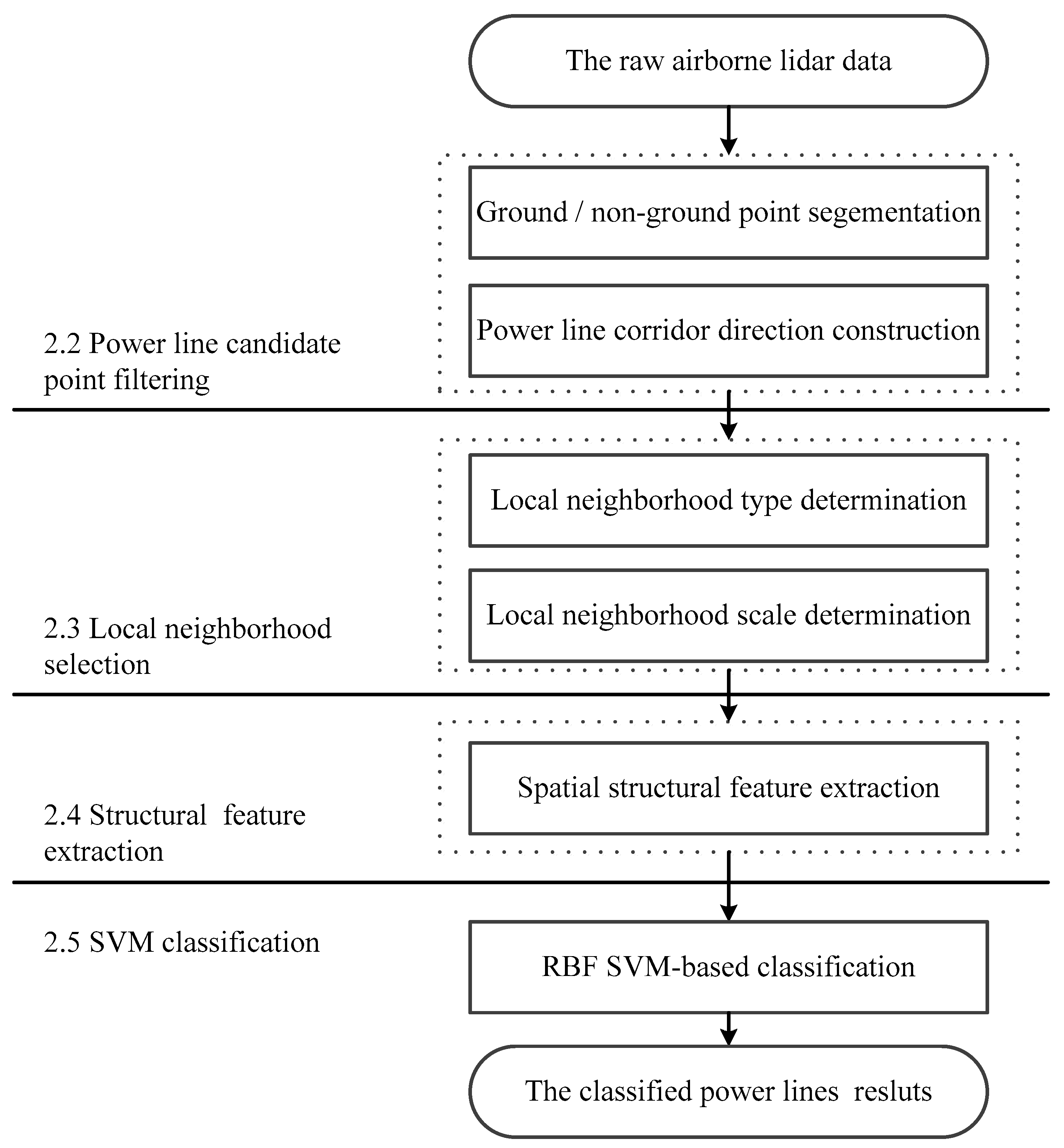
Figure 2.
Visualization of the experimental datasets. (a) the whole large urban LiDAR scene around the campus of the University of Hawaii; (b) the UL (upper left area) Dataset from the blue rectangle in (a); (c) the LP (lower part area) Dataset from the red rectangle in (a). The linear objects of red to orange points are power lines.

Figure 3.
Visualization of power line candidate filtering process. (a) raw LiDAR point cloud; (b) non-ground points; (c) the detected power line 2D corridor direction in XOY plane: the green lines are extracted by Hough transform and the red line is the power line corridor direction constructed by RANSAC algorithm; (d) power line candidate points filtered by power line corridor direction: the red points are true power line points, the blue ones are the power line candidate filtering results.
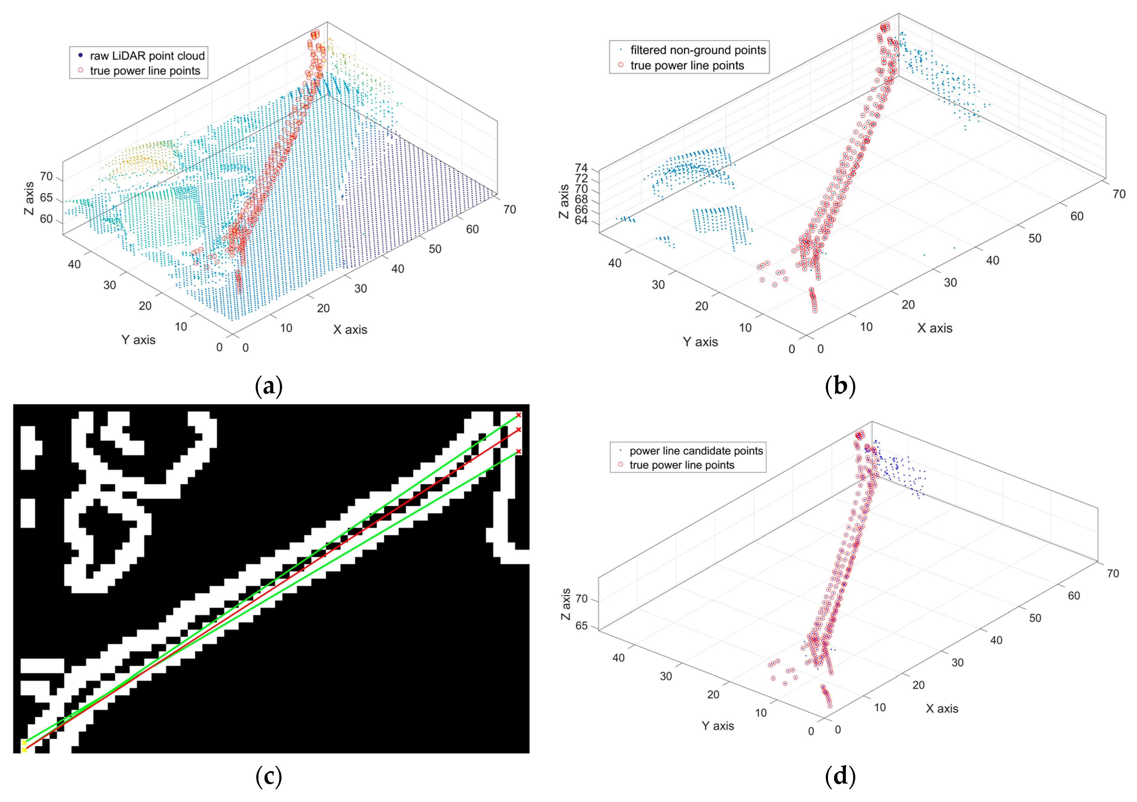
Figure 4.
Visualization of the four different neighborhood types. The black dashed arrow line represents power line corridor direction; the green sphere is the spherical neighborhood of p1 (radius is 5 m); the blue cylinder is the vertical cylindrical neighborhood of p1 (radius is 3 m); blue ‘o’ points are k nearest points of p2 (k = 15); the yellow sphere is k nearest neighborhood of p2 (contains the 15 ‘o’ points); the red cylinder is slant cylindrical neighborhood of p2 (radius is 3 m, height is 12 m, symmetry axis is the corridor direction).

Figure 5.
Visualization of the experiment results for power line classification of UL Dataset. (a) is the whole area results in XOY plane involving the raw LiDAR point cloud, power line candidate points, true power line points and classified power line points; (b) is the local magnification of the blue dashed ellipse area in (a) in power line corridor direction; (c) is the whole area results in 3D view; (d) is the local magnification of the blue dashed ellipse area in (c).
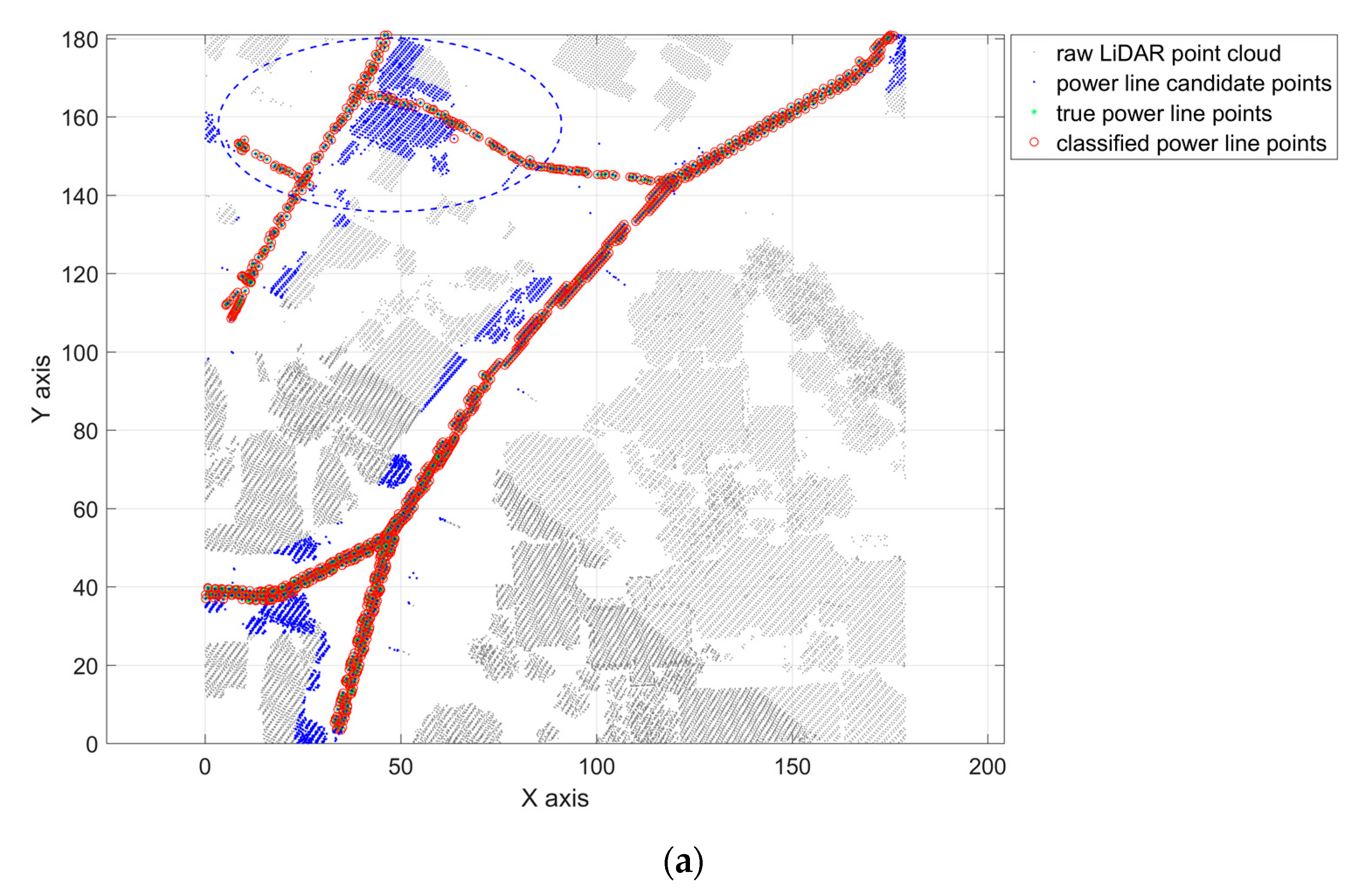

Figure 6.
Visualization of the experiment results for power line classification of LP Dataset. (a) is the whole area results in XOY plane involving the raw LiDAR point cloud, power line candidate points, true power line points and classified power line points; (b) is the local magnification of the blue dashed ellipse area in (a) in power line corridor direction; (c) is the whole area results in 3D view; (d) is the local magnification of the blue dashed ellipse area in (c).

Table 1.
Number of labelled 3D points in the two datasets.
| Class | UL Dataset | LP Dataset |
|---|---|---|
| Ground | 48,070 | 136,891 |
| Building | 24,348 | 48,574 |
| Vegetation | 19,532 | 73,523 |
| Power line | 1519 | 6858 |
| Others (billboard, etc.) | 4475 | 2516 |
| Total | 97,944 | 268,362 |
Table 2.
A partial list of geometric features and distributional features.
| Feature Class | Formal Definition | Computing Method |
|---|---|---|
| Geometric features | Normalized eigenvalues | |
| Linearity | ||
| Planarity | ||
| Scattering | ||
| Distributional features | Omnivariance | |
| Sum | ||
| Changing of curvature | ||
| Radius of local neighborhood | ||
| Density of point set | ||
| Delta of point set in Z axis |
Table 3.
, , (in %) and (in s) for different neighborhood scales and two datasets.
| Scale | UL Dataset | LP Dataset | ||||||
|---|---|---|---|---|---|---|---|---|
| 74.12 | 41.74 | 36.23 | 126 | 79.17 | 58.59 | 50.76 | 1029 | |
| 82.28 | 68.80 | 59.92 | 82 | 93.59 | 63.88 | 61.20 | 935 | |
| 95.19 | 85.91 | 82.33 | 48 | 96.55 | 75.85 | 73.85 | 921 | |
| 95.98 | 91.11 | 87.76 | 44 | 91.99 | 89.59 | 83.11 | 882 | |
| 94.38 | 91.84 | 87.08 | 52 | 93.06 | 91.08 | 85.28 | 942 | |
| 94.65 | 89.73 | 85.40 | 64 | 95.92 | 82.52 | 79.72 | 886 | |
| 97.89 | 94.73 | 92.84 | 131 | 97.98 | 96.85 | 94.95 | 1220 | |
Table 4.
, , (in %) and (in s) for different neighborhood types and two datasets.
| Type | UL Dataset | LP Dataset | ||||||
|---|---|---|---|---|---|---|---|---|
| 97.89 | 94.73 | 92.84 | 131 | 97.98 | 96.85 | 94.95 | 1220 | |
| 97.47 | 96.25 | 93.89 | 152 | 98.19 | 97.42 | 95.70 | 767 | |
| 86.88 | 58.85 | 54.05 | 116 | 87.88 | 79.01 | 71.31 | 1513 | |
| 97.44 | 97.83 | 95.38 | 18 | 98.83 | 98.25 | 97.12 | 98 | |
© 2017 by the authors. Licensee MDPI, Basel, Switzerland. This article is an open access article distributed under the terms and conditions of the Creative Commons Attribution (CC BY) license (http://creativecommons.org/licenses/by/4.0/).
Share and Cite
MDPI and ACS Style
Wang, Y.; Chen, Q.; Liu, L.; Zheng, D.; Li, C.; Li, K. Supervised Classification of Power Lines from Airborne LiDAR Data in Urban Areas. Remote Sens. 2017, 9, 771. https://doi.org/10.3390/rs9080771
AMA Style
Wang Y, Chen Q, Liu L, Zheng D, Li C, Li K. Supervised Classification of Power Lines from Airborne LiDAR Data in Urban Areas. Remote Sensing. 2017; 9(8):771. https://doi.org/10.3390/rs9080771
Chicago/Turabian StyleWang, Yanjun, Qi Chen, Lin Liu, Dunyong Zheng, Chaokui Li, and Kai Li. 2017. "Supervised Classification of Power Lines from Airborne LiDAR Data in Urban Areas" Remote Sensing 9, no. 8: 771. https://doi.org/10.3390/rs9080771
Note that from the first issue of 2016, this journal uses article numbers instead of page numbers. See further details here.