Continental Shelf-Scale Passive Acoustic Detection and Characterization of Diesel-Electric Ships Using a Coherent Hydrophone Array

Abstract
:
1. Introduction
2. Materials and Methods
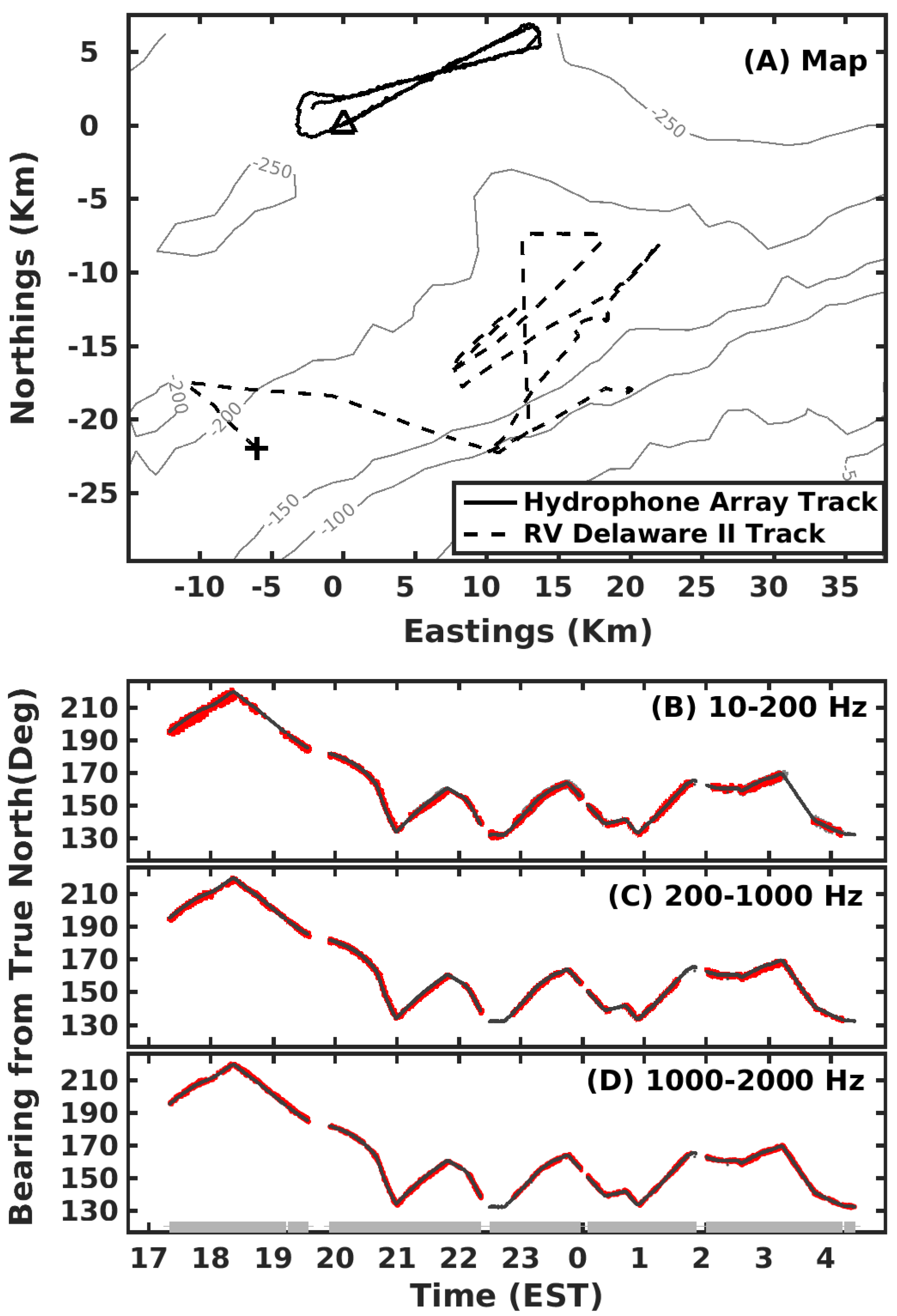
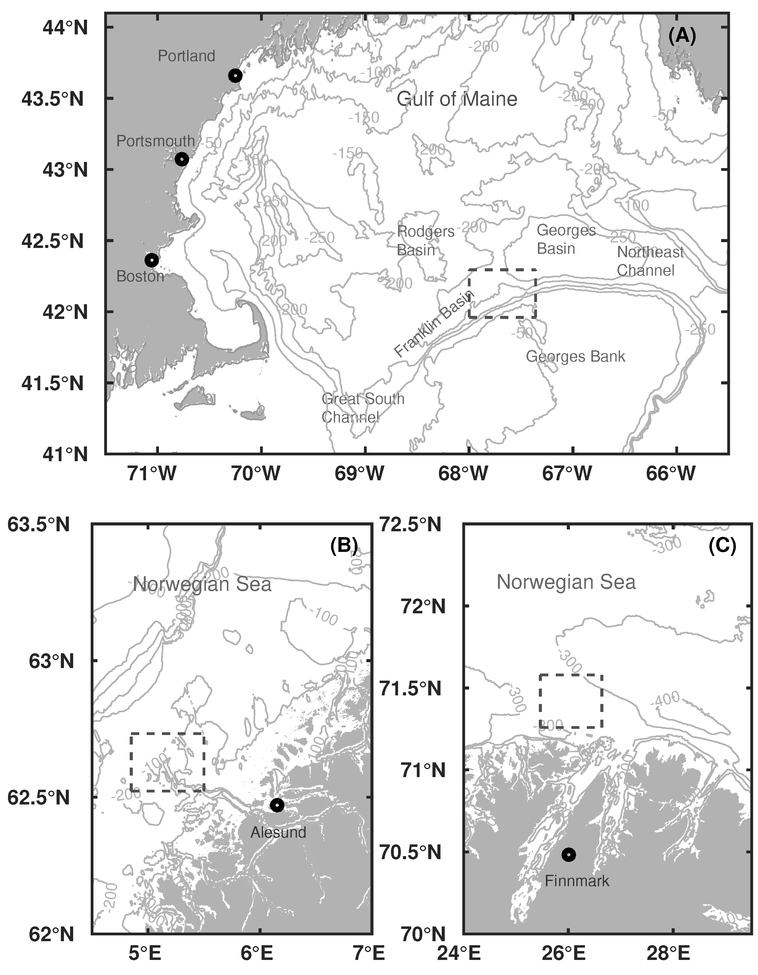
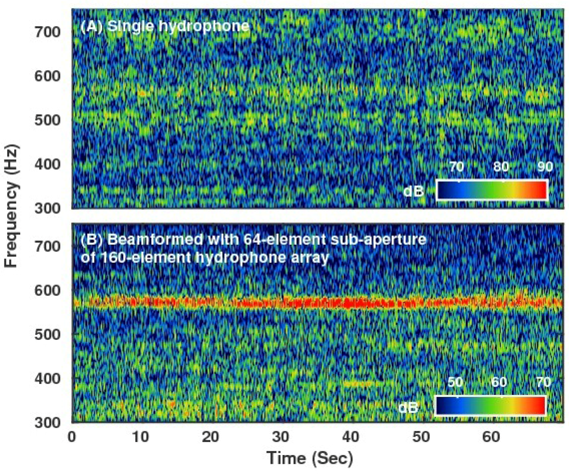
2.1. Measurement of Ship-Radiated Sound Using a Coherent Hydrophone Array
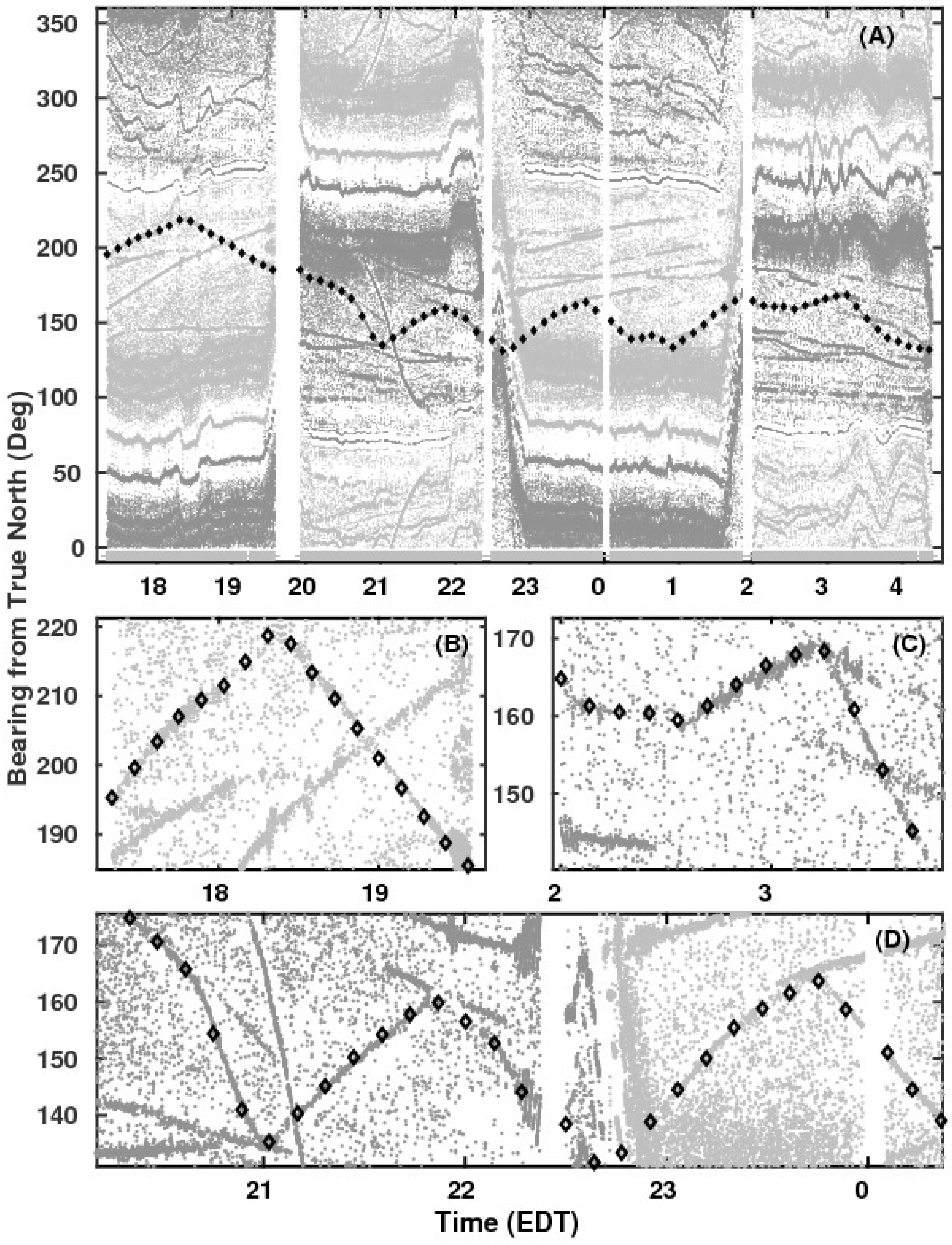
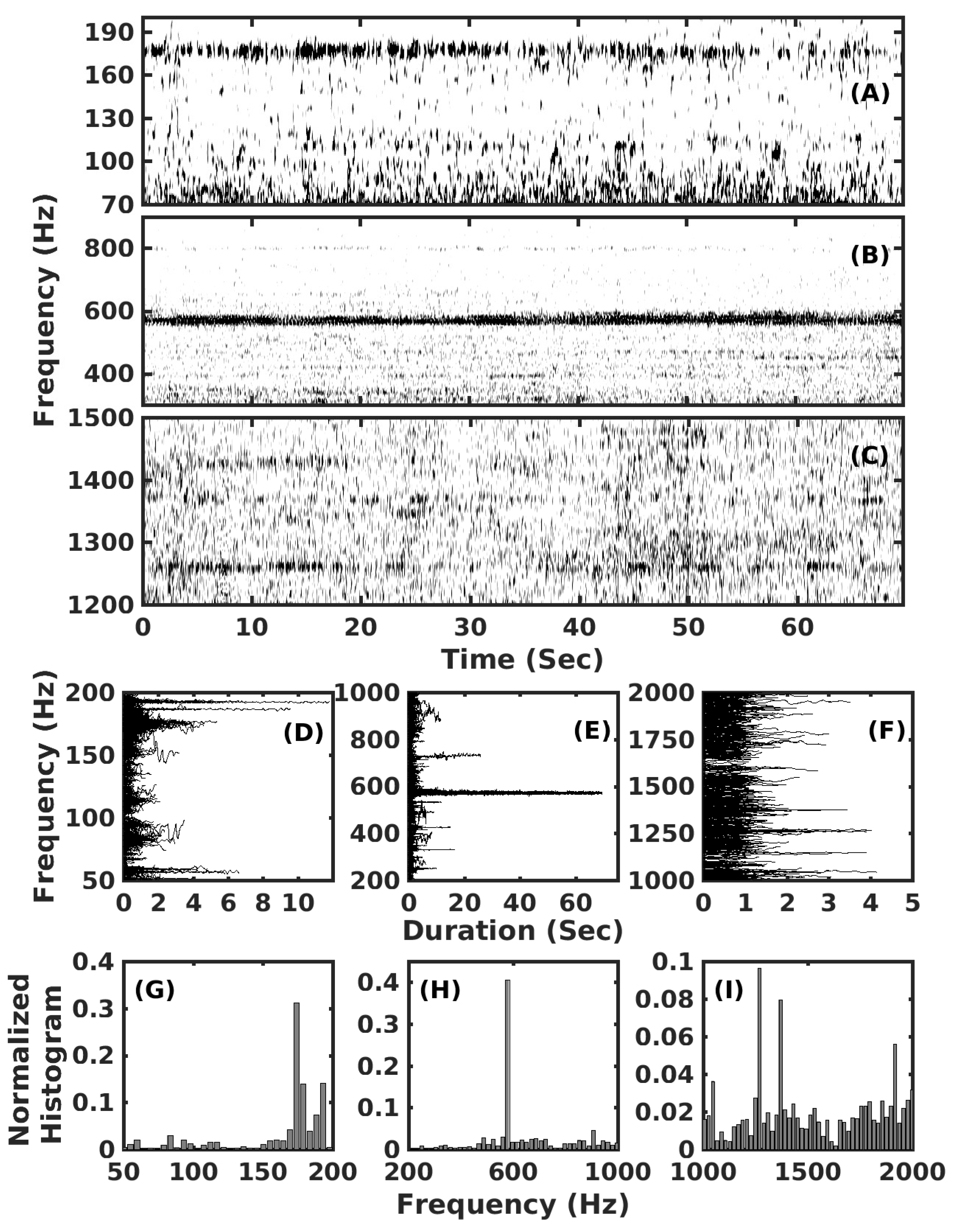
2.2. Ship-Radiated Sound Detection, Bearing Estimation and Characterization
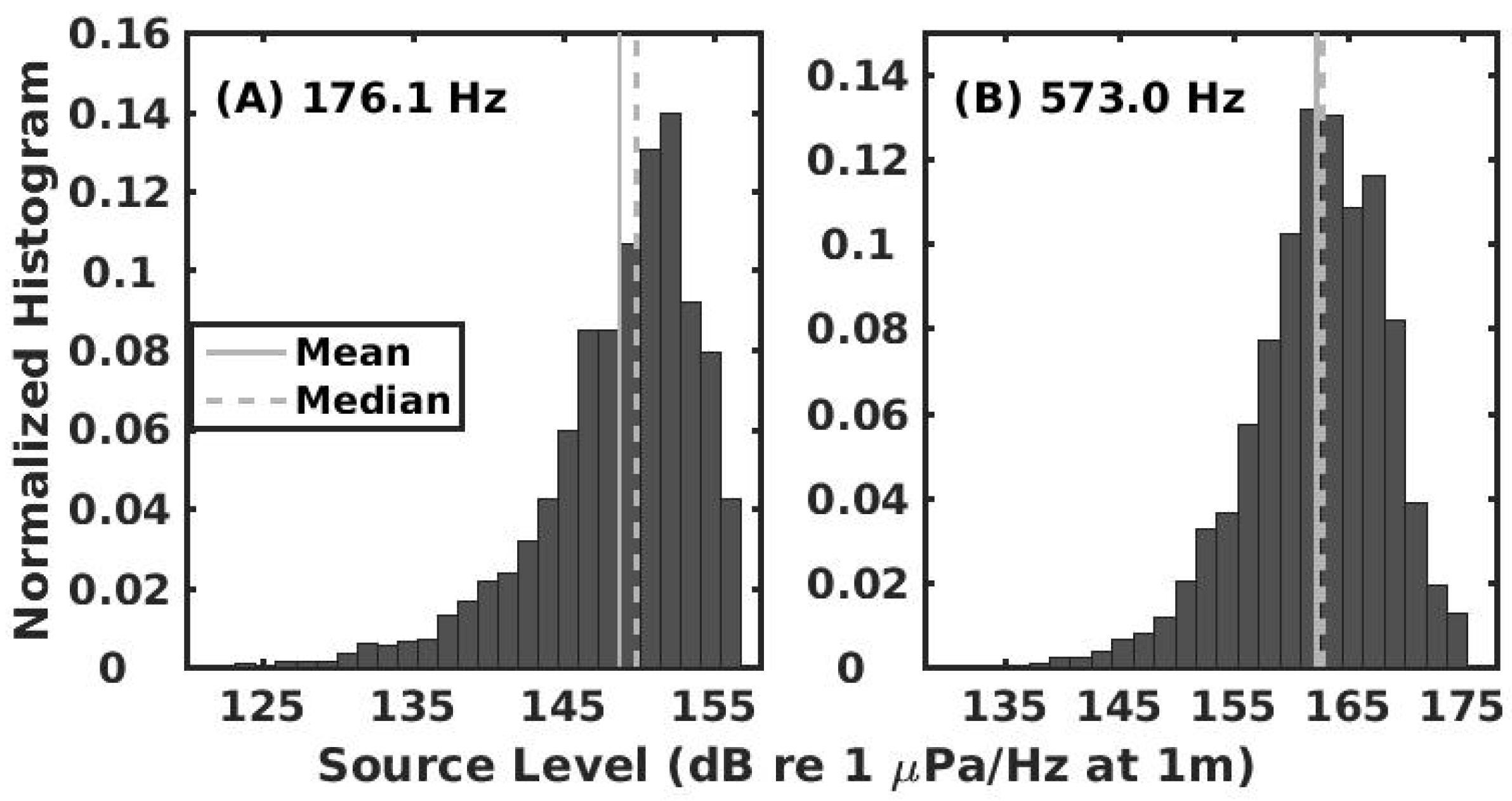
2.3. Source Level Estimation for Ship Tonal and Cyclostationary Signals
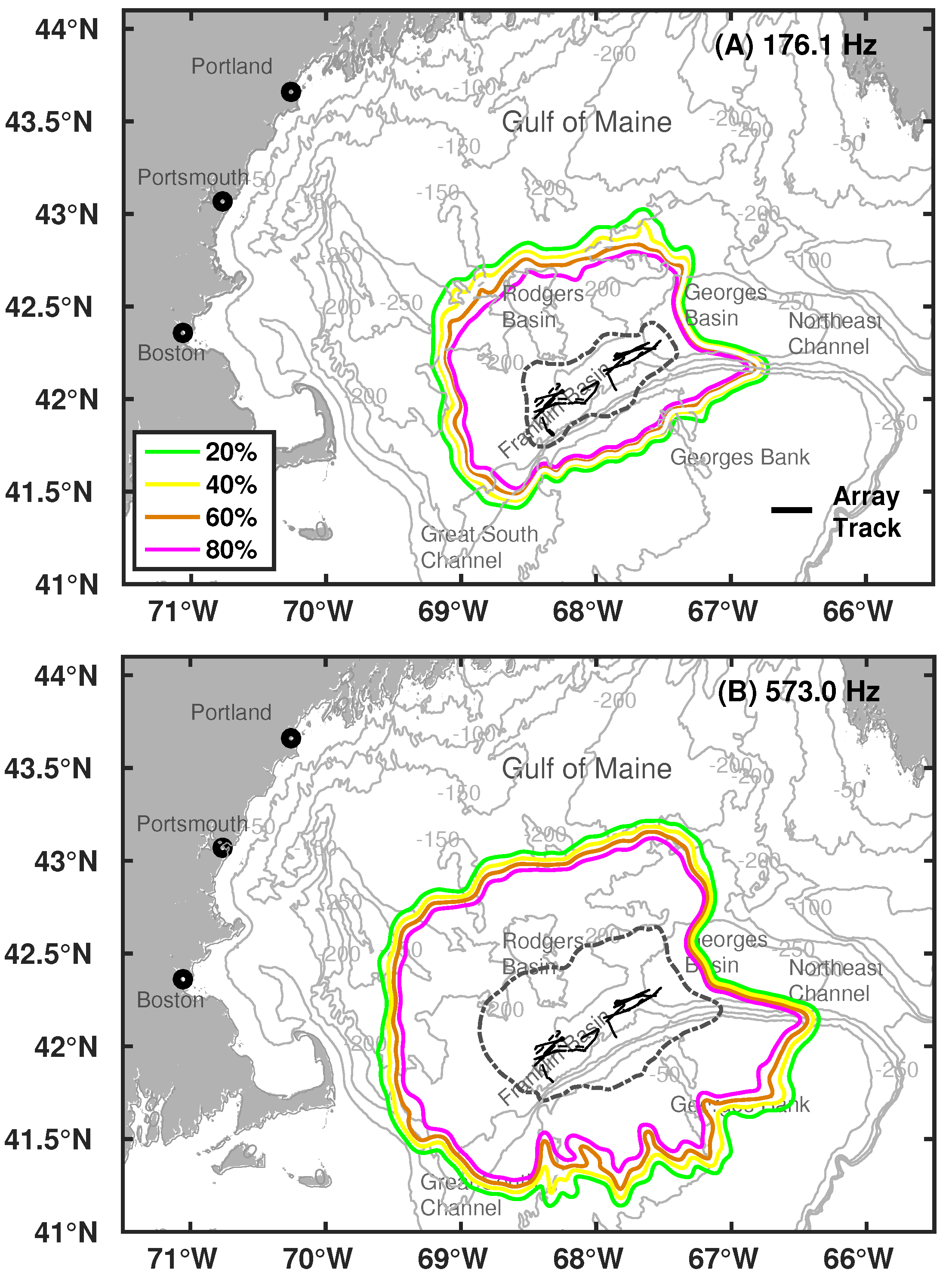
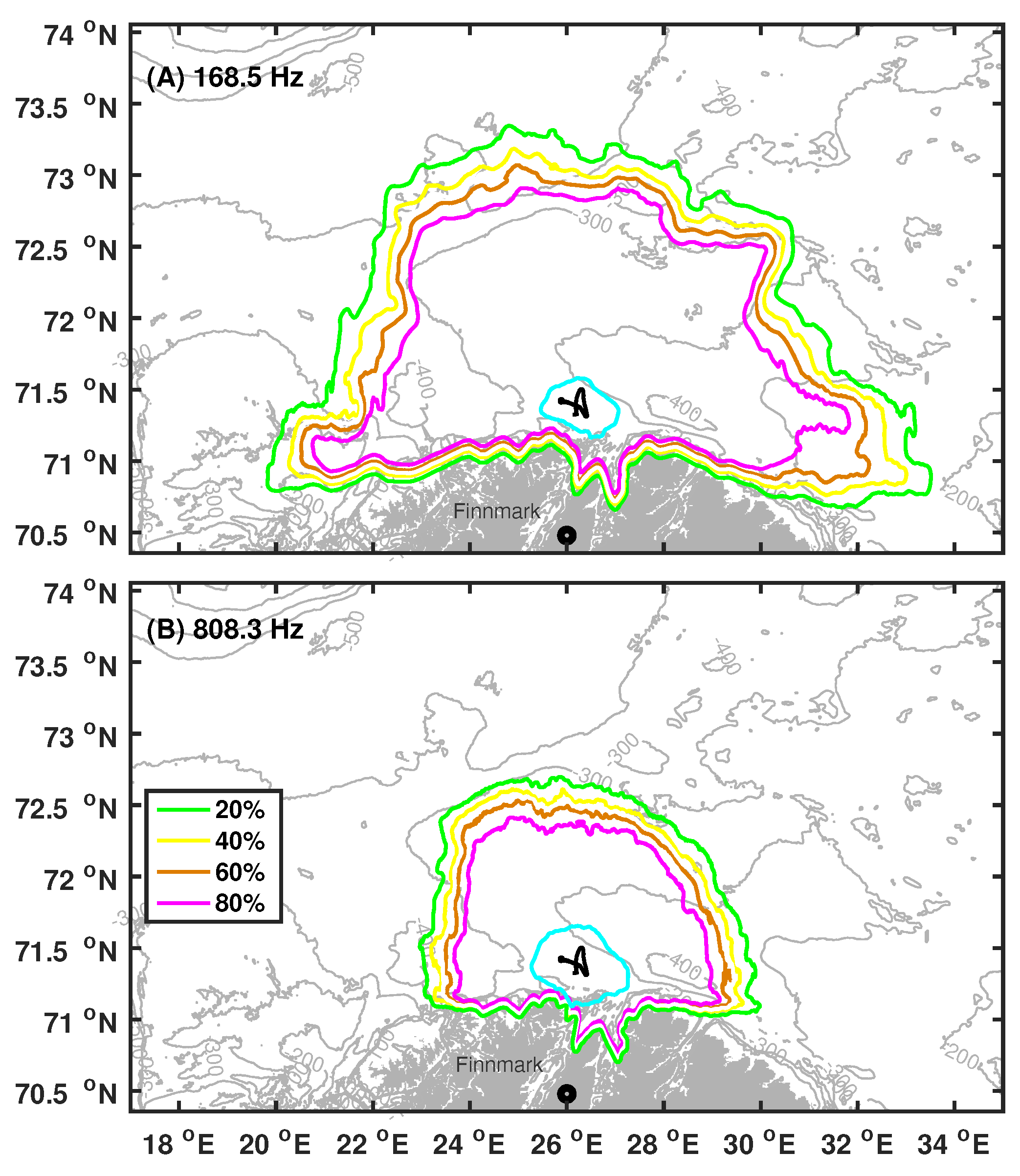
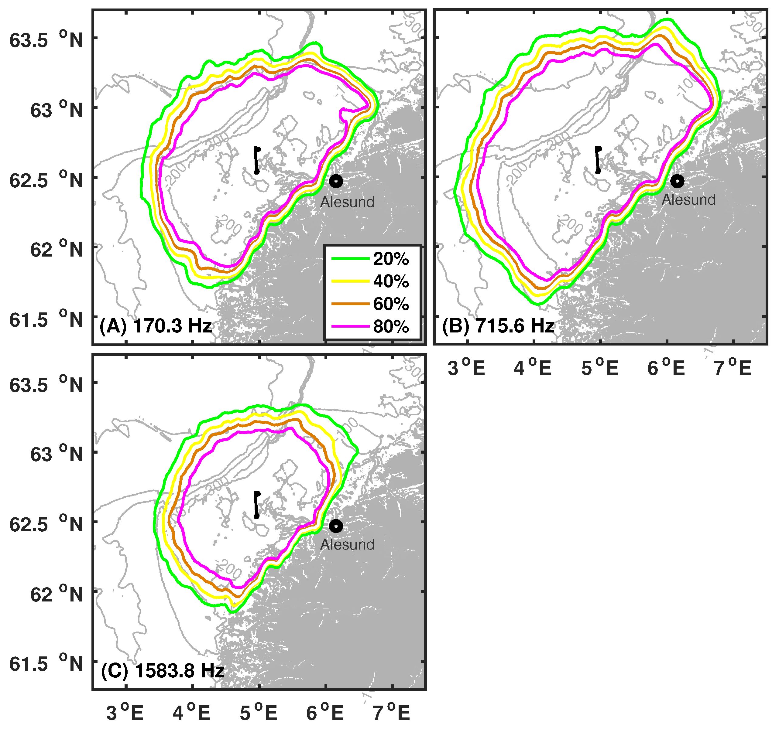
2.4. Probability of Detection Regions for Prominent Ship-Radiated Signals
3. Results
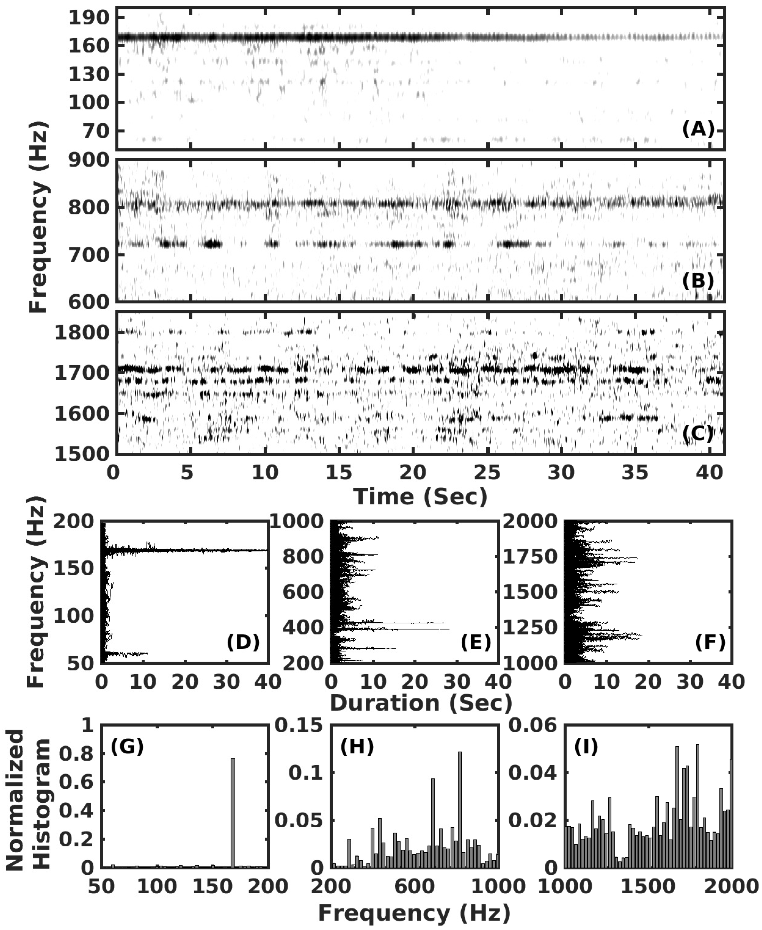
3.1. RV Delaware II
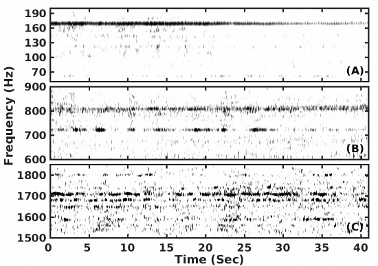
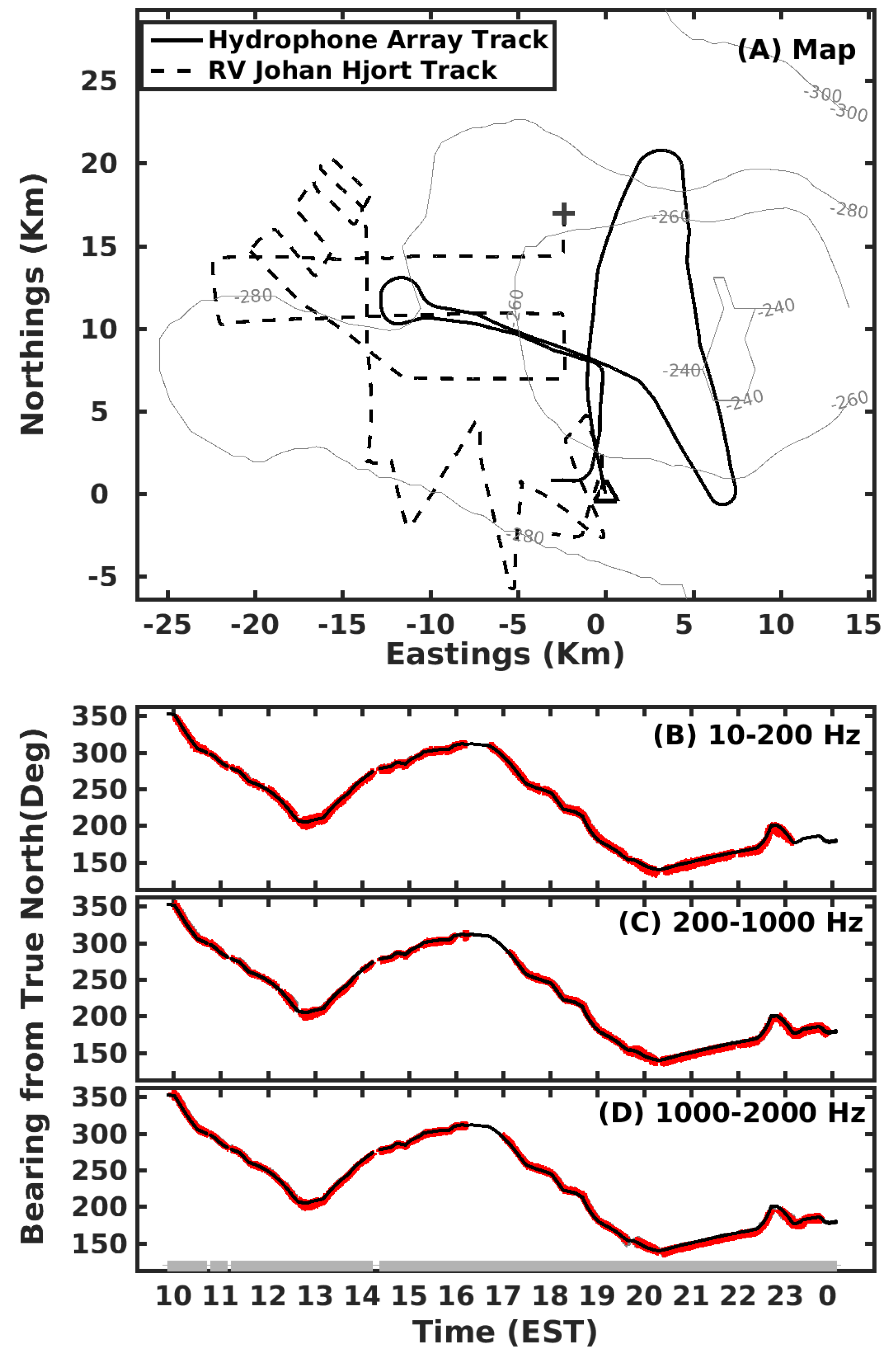
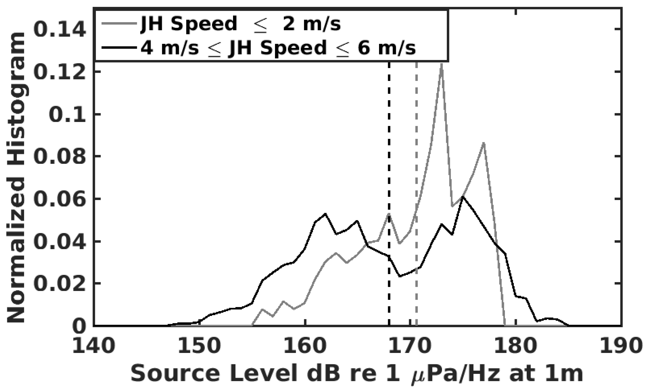
3.2. RV Johan Hjort
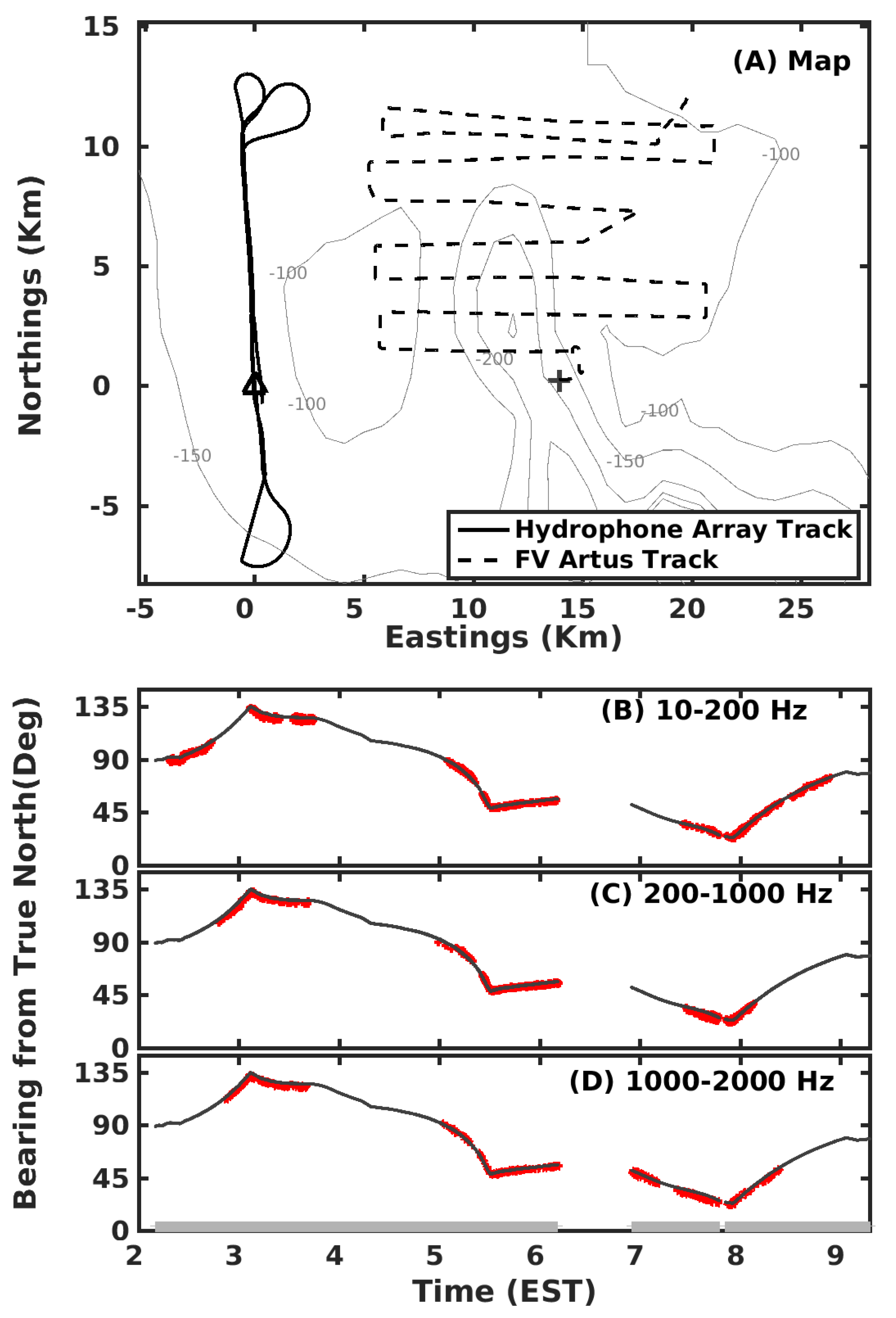
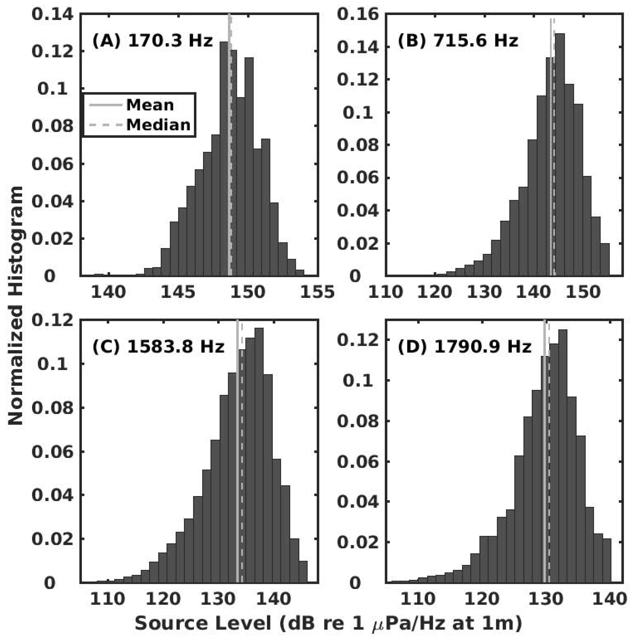
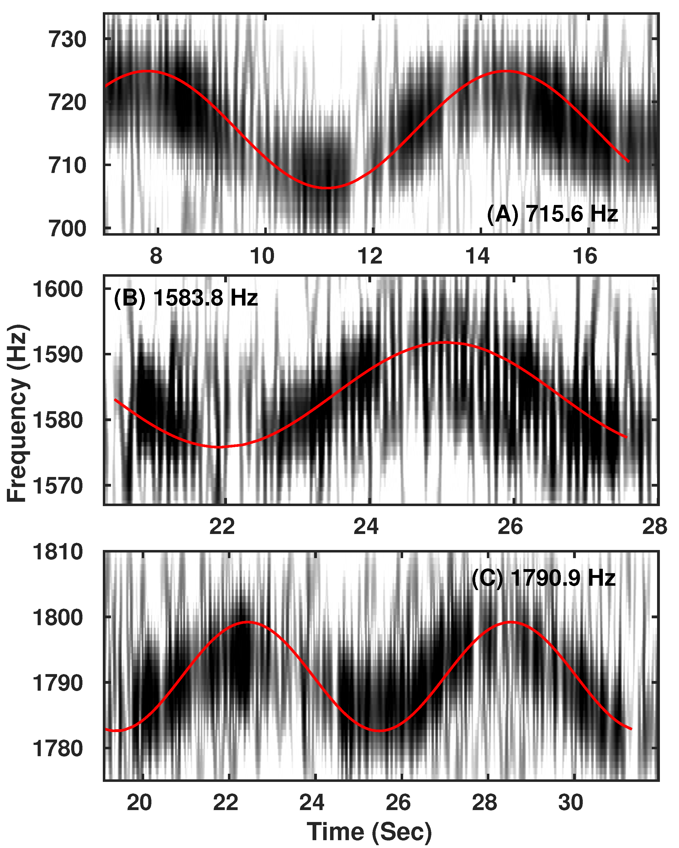
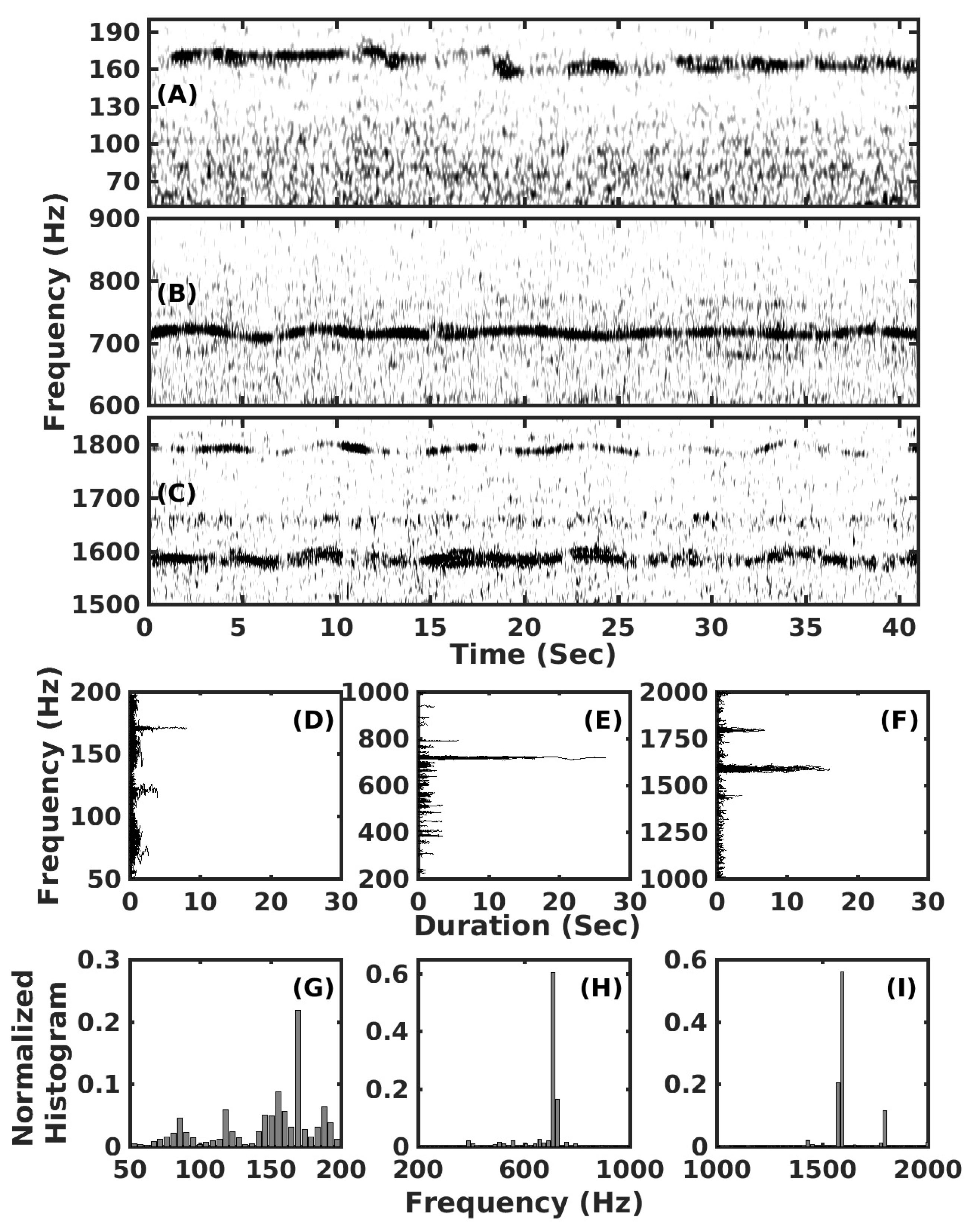
3.3. FV Artus
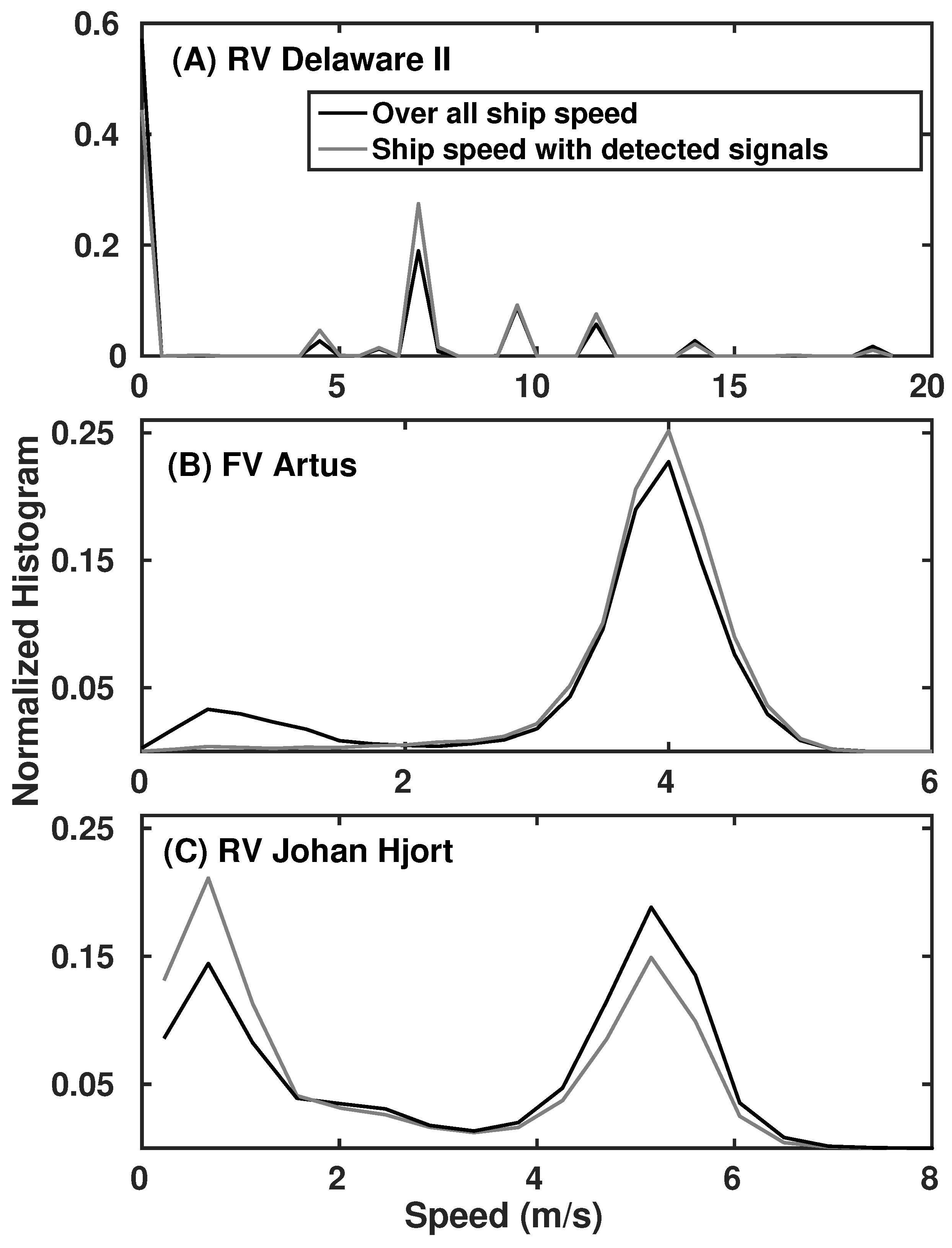
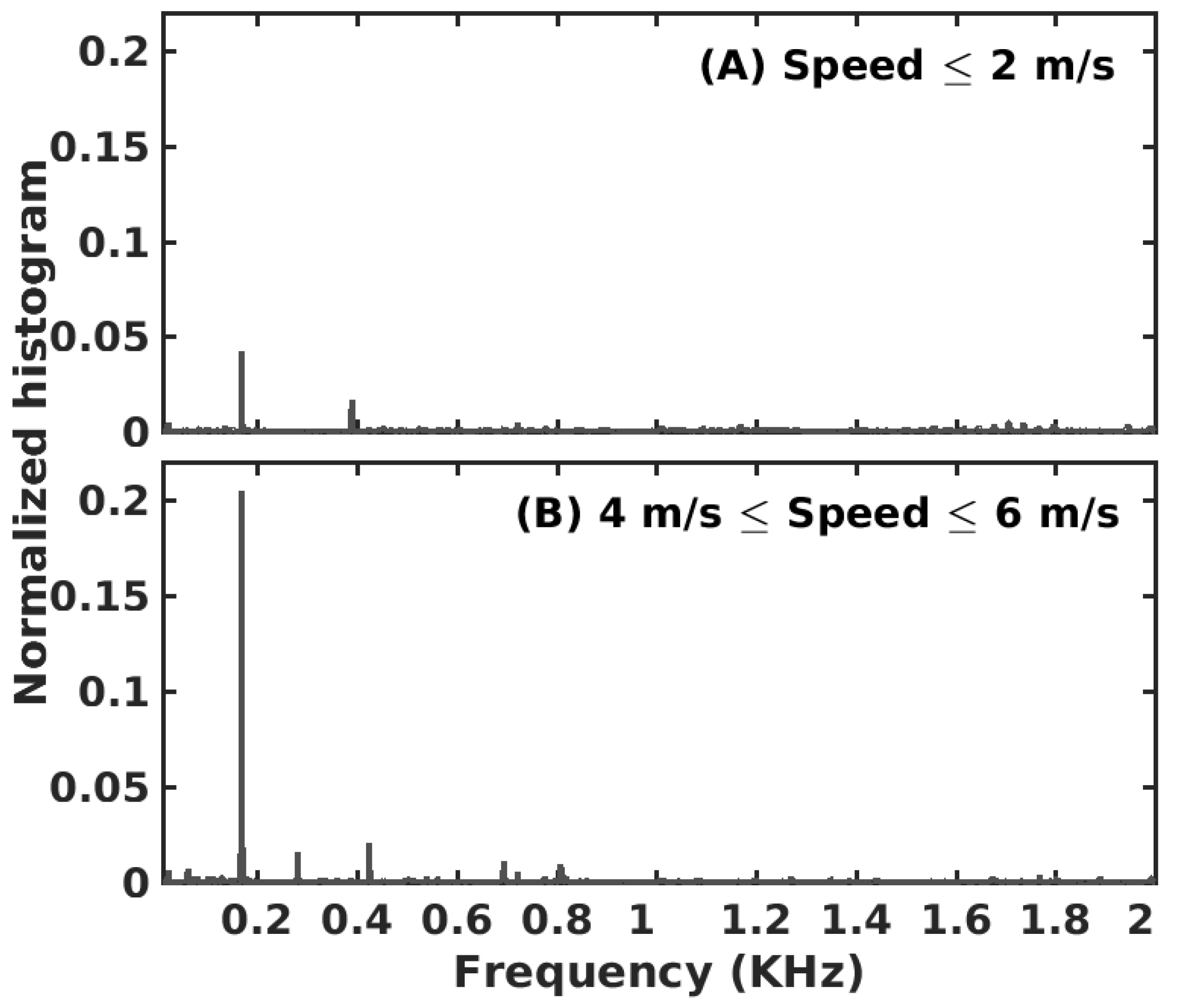
3.4. Dependence of Ship-Radiated Sound on Ship Speed
4. Discussion Including Implications for Studies of Vessel-Induced Fish Behavior
5. Conclusions
Appendix A. Modelling Probability of Detection Regions for Ship-Radiated Signals

| Ships | Frequency | Bandwidth | Ship Signal Source Level | Unbeamformed Ambient Noise Level |
|---|---|---|---|---|
| (Hz) | (Hz) | (dB re 1 μPa/Hz at 1 m) | (dB re 1 μPa/Hz) | |
| RV Delaware II | 176.1 | 3.5 ± 1.7 | 148.7 ± 5.2 | 72.2 |
| 573.0 | 0.8 ± 0.4 | 162.3 ± 6.0 | 67.0 | |
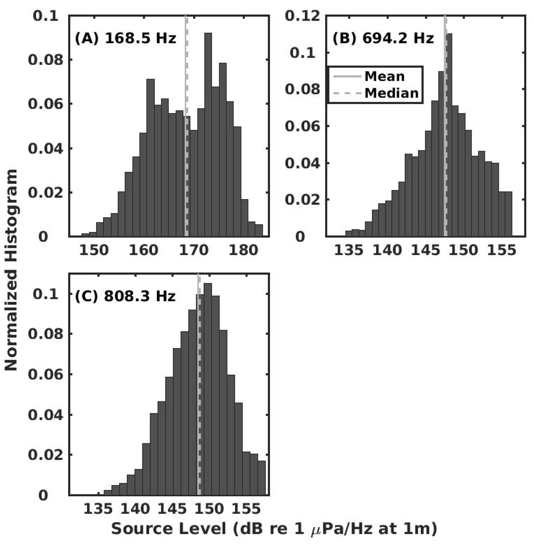
| RV Johan Hjort | 168.5 | 0.8 ± 0.4 | 168.4 ± 7.2 | 86.0 |
| 694.2 | 3.1 ± 1.4 | 147.6 ± 4.3 | 79.0 | |
| 808.3 | 1.9 ± 0.9 | 148.5 ± 4.0 | 77.4 | |
| FV Artus | 170.3 | 1.3 ± 0.9 | 148.7 ± 2.1 | 81.7 |
| 715.6 | 2.5 ± 1.4 | 143.5 ± 5.8 | 76.8 | |
| 1583.8 | 3.4 ± 2.1 | 133.5 ± 6.0 | 70.3 | |
| 1790.9 | 4.0 ± 1.7 | 130.0 ± 5.2 | 67.2 |
Acknowledgments
Author Contributions
Conflicts of Interest
Abbreviations
| POAWRS | passive ocean acoustic waveguide remote sensing |
| OAWRS | ocean acoustic waveguide remote sensing |
| RV | research vessel |
| FV | fishing vessel |
| GPS | global positioning systems |
References
- Bergmann, P.G.; Yaspan, A.; Gerjuoy, E.; Major, J.K.; Wildt, R. (Eds.) Physics of Sound in the Sea; Gordon and Breach: Philadelphia, PA, USA, 1968. [Google Scholar]
- Arveson, P.T.; Vendittis, D.J. Radiated noise characteristics of a modern cargo ship. J. Acoust. Soc. Am. 2000, 107, 118–129. [Google Scholar] [CrossRef] [PubMed]
- Bruno, M.; Chung, K.W.; Salloum, H.; Sedunov, A.; Sedunov, N.; Sutin, A.; Mallas, P. Concurrent use of satellite imaging and passive acoustics for maritime domain awareness. In Proceedings of the 2010 International Waterside Security Conference (WSS), Carrara, Italy, 3–5 November 2010; pp. 1–8. [Google Scholar]
- Chung, K.W.; Sutin, A.; Sedunov, A.; Bruno, M. DEMON acoustic ship signature measurements in an urban harbor. Adv. Acoust. Vib. 2011, 2011, 952798. [Google Scholar] [CrossRef]
- Fillinger, L.; Sutin, A.; Sedunov, A. Acoustic ship signature measurements by cross-correlation method. J. Acoust. Soc. Am. 2010, 129, 774–778. [Google Scholar] [CrossRef] [PubMed]
- Leal, N.; Leal, E.; Sanchez, G. Marine vessel recognition by acoustic signature. ARPN J. Eng. Appl. Sci. 2015, 10. Available online: http://www.arpnjournals.org/jeas/research_papers/rp_2015/jeas_1115_2919.pdf (accessed on 26 July 2017).
- Ogden, G.L.; Zurk, L.M.; Jones, M.E.; Peterson, M.E. Extraction of small boat harmonic signatures from passive sonar. J. Acoust. Soc. Am. 2011, 129, 3768–3776. [Google Scholar] [CrossRef] [PubMed]
- Wales, S.C.; Heitmeyer, R.M. An ensemble source spectra model for merchant ship-radiated noise. J. Acoust. Soc. Am. 2002, 111, 1211–1231. [Google Scholar] [CrossRef] [PubMed]
- Urick, R.J. Principles of Underwater Sound, 3rd ed.; McGraw Hill: New York, NY, USA, 1983; pp. 29–65, 328–366. [Google Scholar]
- Wenz, G.M. Acoustic Ambient Noise in the Ocean: Spectra and Sources. J. Acoust. Soc. Am. 1962, 34, 1936–1956. [Google Scholar]
- Makris, N.C.; Ratilal, P.; Symonds, D.T.; Jagannathan, S.; Lee, S.; Nero, R.W. Fish population and behavior revealed by instantaneous continental shelf-scale imaging. Science 2006, 311, 660–663. [Google Scholar] [CrossRef] [PubMed]
- Makris, N.C.; Ratilal, P.; Jagannathan, S.; Gong, Z.; Andrews, M.; Bertsatos, I.; Godø, O.R.; Nero, R.W.; Jech, J.M. Critical Population Density Triggers Rapid Formation of Vast Oceanic Fish Shoals. Science 2009, 323, 1734–1737. [Google Scholar] [PubMed]
- Wang, D.; Garcia, H.; Huang, W.; Tran, D.D.; Jain, A.D.; Yi, D.H.; Gong, Z.; Jech, J.M.; Godoe, O.R.; Makris, N.C.; et al. Vast assembly of vocal marine mammals from diverse species on fish spawning ground. Nature 2016, 531, 366–370. [Google Scholar] [CrossRef] [PubMed]
- MacLennan, D.N.; Simmonds, E.J. Fisheries Acoustics; Chapman and Hall: London, UK, 1992; Volume 5. [Google Scholar]
- Stojanovic, M. Underwater acoustic communications. In Proceedings of the Professional Program Electro/95 International, Boston, MA, USA, 21–23 June 1995; pp. 435–440. [Google Scholar]
- Stojanovic, M.; Preisig, J. Underwater acoustic communication channels: Propagation models and statistical characterization. IEEE Commun. Mag. 2009, 47, 84–89. [Google Scholar] [CrossRef]
- Dambra, R.; Firenze, E. Underwater Radiated Noise of a Small Vessel. In Proceedings of the 22nd International Congress on Sound and Vibration, Orence, Italy, 12–16 July 2015. [Google Scholar]
- Hildebrand, J.A. Anthropogenic and natural sources of ambient noise in the ocean. Mar. Ecol. Prog. Ser. 2009, 395, 5–20. [Google Scholar] [CrossRef]
- Merchant, N.D.; Witt, M.J.; Blondel, P.; Godley, B.J.; Smith, G.H. Assessing sound exposure from shipping in coastal waters using a single hydrophone and Automatic Identification System (AIS) data. Mar. Pollut. Bull. 2012, 64, 1320–1329. [Google Scholar] [CrossRef] [PubMed]
- Vasconcelos, R.O.; Amorim, M.C.P.; Ladich, F. Effects of ship noise on the detectability of communication signals in the Lusitanian toadfish. J. Exp. Biol. 2007, 210, 2104–2112. [Google Scholar] [CrossRef] [PubMed]
- Codarin, A.; Wysocki, L.E.; Ladich, F.; Picciulin, M. Effects of ambient and boat noise on hearing and communication in three fish species living in a marine protected area (Miramare, Italy). Mar. Pollut. Bull. 2009, 58, 1880–1887. [Google Scholar] [CrossRef] [PubMed]
- Ona, E.; Godø, O.R.; Handegard, N.O.; Hjellvik, V.; Patel, R.; Pedersen, G. Silent research vessels are not quiet. J. Acoust. Soc. Am. 2007, 121, EL145–EL150. [Google Scholar] [CrossRef] [PubMed] [Green Version]
- Mitson, R.B. Underwater noise radiated by research vessels. ICES Mar. Sci. Symp. 1993, 196, 147–152. [Google Scholar]
- Mitson, R.B.; Knudsen, H.P. Causes and effects of underwater noise on fish abundance estimation. Aquat. Living Resour. 2003, 16, 255–263. [Google Scholar] [CrossRef]
- Hatch, L.; Clark, C.; Merrick, R.; Van Parijs, S.; Ponirakis, D.; Schwehr, K.; Thompson, M.; Wiley, D. Characterizing the relative contributions of large vessels to total ocean noise fields: A case study using the Gerry E. Studds Stellwagen Bank National Marine Sanctuary. Environ. Manag. 2008, 42, 735–752. [Google Scholar] [CrossRef] [PubMed]
- Veirs, S.; Veirs, V.; Wood, J.D. Ship noise extends to frequencies used for echolocation by endangered killer whales. PeerJ 2016, 4, e1657. [Google Scholar] [CrossRef] [PubMed]
- Wittekind, D.K. A simple model for the underwater noise source level of ships. J. Ship Rrod. Design 2014, 30, 7–14. [Google Scholar]
- Mitson, R.B. Underwater Noise of Research Vessels; ICES Co-Operative Research Report; ICES: Copenhagen, Denmark, 1995; Volume 61. [Google Scholar]
- Fernandes, P.G.; Brierley, A.S.; Simmonds, E.J.; Millard, N.W.; McPhail, S.D.; Armstrong, F.; Stevenson, P.; Squires, M. Oceanography: Fish do not avoid survey vessels. Nature 2000, 404, 35–36. [Google Scholar] [CrossRef] [PubMed]
- Jørgensen, R.; Handegard, N.O.; Gjøsæter, H.; Slotte, A. Possible vessel avoidance behaviour of capelin in a feeding area and on a spawning ground. Fish. Res. 2004, 69, 251–261. [Google Scholar] [CrossRef]
- De Robertis, A.; Handegard, N.O. Fish avoidance of research vessels and the efficacy of noise-reduced vessels: A review. ICES J. Mar. Sci. 2013, 70, 34–45. [Google Scholar] [CrossRef]
- Huang, W.; Wang, D.; Ratilal, P. Diel and Spatial Dependence of Humpback Song and Non-Song Vocalizations in Fish Spawning Ground. Remote Sens. 2016, 8, 712. [Google Scholar] [CrossRef]
- Gong, Z.; Jain, A.D.; Tran, D.D.; Yi, D.H.; Wu, F.; Zorn, A.; Ratilal, P.; Makris, N.C. Ecosystem scale acoustic sensing reveals humpback whale behavior synchronous with herring spawning processes and re-evaluation finds no effect of sonar on humpback song occurrence in the Gulf of Maine in Fall 2006. PLoS ONE 2014, 9, e104733. [Google Scholar] [CrossRef] [PubMed]
- Tran, D.D.; Huang, W.; Bohn, A.C; Wang, D.; Gong, Z.; Makris, N.C; Ratilal, P. Using a coherent hydrophone array for observing sperm whale range, classification, and shallow-water dive profiles. J. Acoust. Soc. Am. 2014, 135, 3352–3363. [Google Scholar] [CrossRef] [PubMed]
- Wang, D.; Huang, W.; Garcia, H.; Ratilal, P. Vocalization source level distributions and pulse compression gains of diverse baleen whale species in the Gulf of Maine. Remote Sens. 2016, 8, 881. [Google Scholar] [CrossRef]
- Crocker, S.E.; Nielsen, P.L.; Miller, J.H.; Siderius, M. Geoacoustic inversion of ship radiated noise in shallow water using data from a single hydrophone. J. Acoust. Soc. Am. 2014, 136, EL362–EL368. [Google Scholar] [CrossRef] [PubMed]
- Hallett, M.A. Characteristics of merchant ship acoustic signatures during port entry/exit. In Proceedings of the Acoustics, Gold Coast, Australia, 3–5 November 2004; pp. 3–5. [Google Scholar]
- Sutin, A.; Bunin, B.; Sedunov, A.; Sedunov, N.; Fillinger, L.; Tsionskiy, M.; Bruno, M. Stevens passive acoustic system for underwater surveillance. In Proceedings of the 2010 International Waterside Security Conference (WSS), Carrara, Italy, 3–5 November 2010; pp. 1–6. [Google Scholar]
- Nejedl, V.; Stoltenberg, A.; Schulz, J. Free-field measurements of the radiated and structure borne sound of RV Planet. Proc. Meet. Acoust. 2012, 17, 070061. [Google Scholar] [CrossRef]
- McKenna, M.F.; Ross, D.; Wiggins, S.M.; Hildebrand, J.A. Underwater radiated noise from modern commercial ships. J. Acoust. Soc. Am. 2012, 131, 92–103. [Google Scholar] [CrossRef] [PubMed]
- Fréchou, D.; Dugué, C.; Briançon-Marjollet, L.; Fournier, P.; Darquier, M.; Descotte, L.; Merle, L. Marine Propulsor Noise Investigations in the Hydroacoustic Water Tunnel “GTH”. In Proceedings of the Twenty-Third Symposium on Naval Hydrodynamics, Val de Reuil , France, 17–22 September 2000. [Google Scholar]
- Bush, V.; Conant, J.B.; Tate, J.T. Principles and Applications of Underwater Sound; Summary Technical Report; Office of Scientific Research and Development: Washington, DC, USA, 1946; Volume 7. [Google Scholar]
- Norwood, C. An introduction to ship radiated noise. Acoust. Aust. 2002, 30, 21–25. [Google Scholar]
- Ojak, W. Vibrations and waterborne noise on fishery vessels. J. Ship Res. 1988, 32, 112–133. [Google Scholar]
- Gray, L.M.; Greeley, D.S. Source level model for propeller blade rate radiation for the world’s merchant fleet. J. Acoust. Soc. Am. 1980, 67, 516–522. [Google Scholar] [CrossRef]
- Grelowska, G.; Kozaczka, E.; Kozaczka, S.; Szymczak, W. Underwater noise generated by a small ship in the shallow sea. Arch. Acoust. 2013, 38, 351–356. [Google Scholar] [CrossRef]
- Malinowski, S.J.; Gloza, I. Underwater noise characteristics of small ships. Acta Acust. United Acust. 2002, 88, 718–721. [Google Scholar]
- Gloza, I. Identification methods of underwater noise sources generated by small ships. Acta Phys. Pol. A 2011, 119, 961–965. [Google Scholar] [CrossRef]
- Gloza, I.; Malinowski, S. Identification of ships underwater noise sources in the coastal region. Hydroacoustics 2003, 5, 9–16. [Google Scholar]
- Sandhya, M.; Rajarajeswari, K.; Seetaramaiah, P. Detecting Inception of Hydrodynamic cavitation Noise of Ships using Quadratic Phase coupling Index as an Indicator. Def. Sci. J. 2015, 65, 53–62. [Google Scholar] [CrossRef]
- Trevorrow, M.V.; Vasiliev, B.; Vagle, S. Directionality and maneuvering effects on a surface ship underwater acoustic signature. J. Acoust. Soc. Am. 2008, 124, 767–778. [Google Scholar] [CrossRef] [PubMed]
- Ianniello, S.; Muscari, R.; Di Mascio, A. Ship underwater noise assessment by the acoustic analogy. Part I: Nonlinear analysis of a marine propeller in a uniform flow. J. Mar. Sci. Technol. 2013, 18, 547–570. [Google Scholar] [CrossRef]
- Shioiri, An Aspect of the Propeller-Singing Phenomenon as a Self-Excited Oscillation. Davidson Laboratory Report 1059. Available online: http://www.dtic.mil/get-tr-doc/pdf?AD=AD0464615 (accessed on 26 July 2017).
- Andrews, M.; Chen, T.; Ratilal, P. Empirical dependence of acoustic transmission scintillation statistics on bandwidth, frequency and range in New Jersey continental shelf. J. Acoust. Soc. Am. 2009, 125, 111–124. [Google Scholar] [CrossRef] [PubMed]
- Andrews, M.; Gong, Z.; Ratilal, P. Effects of multiple scattering, attenuation and dispersion in waveguide sensing of fish. J. Acoust. Soc. Am. 2011, 130, 1253–1272. [Google Scholar] [CrossRef] [PubMed]
- Gong, Z.; Andrews, M.; Jagannathan, S.; Patel, R.; Jech, J.M.; Makris, N.C.; Ratilal, P. Low-frequency target strength and abundance of shoaling Atlantic herring (Clupea harengus) in the Gulf of Maine during the Ocean Acoustic Waveguide Remote Sensing 2006 Experiment. J. Acoust. Soc. Am. 2010, 127, 104–123. [Google Scholar] [CrossRef] [PubMed]
- Tran, D.; Andrews, M.; Ratilal, P. Probability distribution for energy of saturated broadband ocean acoustic transmission: Results from Gulf of Maine 2006 experiment. J. Acoust. Soc. Am. 2012, 132, 3659–3672. [Google Scholar] [CrossRef] [PubMed]
- Collins, M.D. A split step Padé solution for the parabolic equation method. J. Acoust. Soc. Am. 1993, 93, 1736–1742. [Google Scholar] [CrossRef]
- Collins, M.D.; Westwood, E. K. A higher-order energy-conserving parabolic equqation for range-dependent ocean depth, sound speed, and density. J. Acoust. Soc. Am. 1991, 89, 1068–1075. [Google Scholar] [CrossRef]
- Gong, Z.; Tran, D.D.; Ratilal, P. Comparing passive source localization and tracking approaches with a towed horizontal receiver array in an ocean waveguide. J. Acoust. Soc. Am. 2013, 134, 3705–3720. [Google Scholar] [CrossRef] [PubMed]
- Jagannathan, S.; Kusel, E.T.; Ratilal, P.; Makris, N.C. Scattering from extended targets in range-dependent fluctuating ocean-waveguides with clutter from theory and experiments. J. Acoust. Soc. Am. 2012, 132, 680–693. [Google Scholar] [CrossRef] [PubMed]
- Jagannathan, S.; Bertsatos, I.; Symonds, D.; Chen, T.; Nia, H.T.; Jain, A.D.; Jech, M. Ocean acoustic waveguide remote sensing (OAWRS) of marine ecosystems. MEPS 2009, 395, 137–160. [Google Scholar] [CrossRef]
- Overholtz, W.J.; Jech, J.M.; Michaels, W. L.; Jacobson, L.D.; Sullivan, P.J. Empirical comparisons of survey designs in acoustic surveys of Gulf of Maine-Georges Bank Atlantic herring. J. Northw. Atl. Fish. Sci. 2006, 36, 127–144. [Google Scholar] [CrossRef]
- Weinberg, J. 54th Northeast Regional Stock Assessment Workshop (54th SAW) Assessment Report; Northeast Fisheries Science Center Reference Document 12-18; Northeast Fisheries Science Center: Woods Hole, MA, USA, 2012. [Google Scholar]
- Jech, J.M.; Stroman, F. Aggregative patterns of pre-spawning Atlantic herring on Georges Bank from 1999–2010. Aquat. Living Resour. 2012, 25, 1–14. [Google Scholar] [CrossRef]
- Becker, K.; Preston, J.R. The ONR Five Octave Research Array (FORA) at Penn State. IEEE J. Ocean Eng. 2003, 5, 2607–2610. [Google Scholar]
- Ratilal, P.; Lai, Y.S.; Symonds, D.T.; Ruhlmann, L.A.; Preston, J.R.; Scheer, E.K.; Garr, M.T.; Holland, C.W.; Goff, J.A.; Makris, N.C. Long range acoustic imaging of the continental shelf environment: The Acoustic Clutter Reconnaissance Experiment 2001. J. Acoust. Soc. Am. 2005, 1117, 1977–1998. [Google Scholar] [CrossRef]
- Jain, A.D. Instantaneous Continental-Shelf Scale Sensing of Cod with Ocean Acoustic Waveguide Remote Sensing (OAWRS). Ph.D. Thesis, Massachusetts Institute of Technology, Cambridge, MA, USA, 2015. [Google Scholar]
- Kay, S.M. Fundamentals of Statistical Signal Processing, Volume II: Detection Theory; Prentice-Hall: Upper Saddle River, NJ, USA, 1993; pp. 375–380. [Google Scholar]
- Johnson, D.H.; Dudgeon, D.E. Array Signal Processing: Concepts and Techniques; Simon & Schuster: New York, NY, USA, 1992; pp. 1–512. [Google Scholar]
- Baumgartner, M.F.; Mussoline, S.E. A generalized baleen whale call detection and classification system. J. Acoust. Soc. Am. 2011, 129, 2889–2902. [Google Scholar] [CrossRef] [PubMed]
- Shapiro, A.D.; Wang, C. A versatile pitch tracking algorithm: From human speech to killer whale vocalizations. J. Acoust. Soc. Am. 2009, 126, 451–459. [Google Scholar] [CrossRef] [PubMed]
- Kinsler, L.E.; Frey, A.R.; Coppens, A.B.; Sanders, J.V. Fundamentals of Acoustics, 4th ed.; Wiley-VCH: New York, NY, USA, 1999; p. 448. [Google Scholar]
- Da Costa, E.L. Detection and Identification of Cyclostationary Signals; Naval Postgraduate School: Monterey, CA, USA, 2007. [Google Scholar]
- Blake, W. K. Periodic and random excitation of streamlined structures by trailing edge flows. In Turbulence in Liquids; Science Press: Princeton, NJ, USA, 1977; pp. 167–178. [Google Scholar]
- Burdic, W.S. Underwater Acoustic System Analysis; Prentice Hall: Upper Saddle River, NJ, USA, 1991; pp. 322–360. [Google Scholar]
- Clay, C. S.; Medwin, H. Acoustical Oceanography: Principles and Applications; John Wiley & Sons: New York, NY, USA, 1977; pp. 494–501. [Google Scholar]
- Jensen, F.B.; Kuperman, W.A.; Porter, M.B.; Schmidt, H. Computational Ocean Acoustics, 2nd ed.; Springer Science & Business Media: Berlin, Germany, 2011; pp. 708–713. [Google Scholar]
- DiFranco, J.V.; Rubin, W.L. Radar Detection; Artech House Inc.: Dedham, MA, USA, 1980. [Google Scholar]
- Makris, N.C. The effect of saturated transmission scintillation on ocean acoustic intensity measurements. J. Acoust. Soc. Am. 1996, 100, 769–783. [Google Scholar] [CrossRef]


| B | ||
|---|---|---|
| (Hz) | (Hz) | (Hz) |
| 715.6 | 9.3 | 0.15 |
| 1583.8 | 8.0 | 0.16 |
| 1790.9 | 8.3 | 0.164 |
© 2017 by the authors. Licensee MDPI, Basel, Switzerland. This article is an open access article distributed under the terms and conditions of the Creative Commons Attribution (CC BY) license (http://creativecommons.org/licenses/by/4.0/).
Share and Cite
Huang, W.; Wang, D.; Garcia, H.; Godø, O.R.; Ratilal, P. Continental Shelf-Scale Passive Acoustic Detection and Characterization of Diesel-Electric Ships Using a Coherent Hydrophone Array. Remote Sens. 2017, 9, 772. https://doi.org/10.3390/rs9080772
Huang W, Wang D, Garcia H, Godø OR, Ratilal P. Continental Shelf-Scale Passive Acoustic Detection and Characterization of Diesel-Electric Ships Using a Coherent Hydrophone Array. Remote Sensing. 2017; 9(8):772. https://doi.org/10.3390/rs9080772
Chicago/Turabian StyleHuang, Wei, Delin Wang, Heriberto Garcia, Olav Rune Godø, and Purnima Ratilal. 2017. "Continental Shelf-Scale Passive Acoustic Detection and Characterization of Diesel-Electric Ships Using a Coherent Hydrophone Array" Remote Sensing 9, no. 8: 772. https://doi.org/10.3390/rs9080772