
Estimating Daily Reference Evapotranspiration in a Semi-Arid Region Using Remote Sensing Data


1
Centre for Landscape and Climate Research, School of Geography, Geology and the Environment, University of Leicester, Leicester LE1 7RH, UK
2
Department of Soil and Water Science, Faculty of Agricultural Sciences, University of Sulaimani, Iraq-Kurdistan Region-Sulaimani-Bekrajo 46011, Iraq
3
National Centre for Earth Observation, University of Leicester, Leicester LE1 7RH, UK
*
Author to whom correspondence should be addressed.
Remote Sens. 2017, 9(8), 779; https://doi.org/10.3390/rs9080779
Submission received: 19 May 2017
/
Revised: 26 July 2017
/
Accepted: 27 July 2017
/
Published: 29 July 2017
(This article belongs to the Special Issue Remote Sensing of Arid/Semiarid Lands)
Abstract
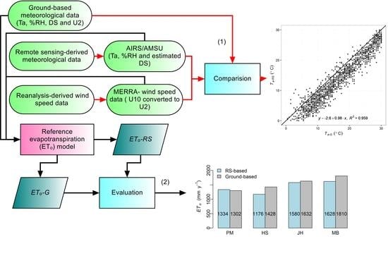
:Estimating daily evapotranspiration is challenging when ground observation data are not available or scarce. Remote sensing can be used to estimate the meteorological data necessary for calculating reference evapotranspiration ETₒ. Here, we assessed the accuracy of daily ETₒ estimates derived from remote sensing (ETₒ-RS) compared with those derived from four ground-based stations (ETₒ-G) in Kurdistan (Iraq) over the period 2010–2014. Near surface air temperature, relative humidity and cloud cover fraction were derived from the Atmospheric Infrared Sounder/Advanced Microwave Sounding Unit (AIRS/AMSU), and wind speed at 10 m height from MERRA (Modern-Era Retrospective Analysis for Research and Application). Four methods were used to estimate ETₒ: Hargreaves–Samani (HS), Jensen–Haise (JH), McGuinness–Bordne (MB) and the FAO Penman Monteith equation (PM). ETₒ-G (PM) was adopted as the main benchmark. HS underestimated ETₒ by 2%–3% (R2 = 0.86 to 0.90; RMSE = 0.95 to 1.2 mm day−1 at different stations). JH and MB overestimated ETₒ by 8% to 40% (R2 = 0.85 to 0.92; RMSE from 1.18 to 2.18 mm day−1). The annual average values of ETₒ estimated using RS data and ground-based data were similar to one another reflecting low bias in daily estimates. They ranged between 1153 and 1893 mm year−1 for ETₒ-G and between 1176 and 1859 mm year−1 for ETₒ-RS for the different stations. Our results suggest that ETₒ-RS (HS) can yield accurate and unbiased ETₒ estimates for semi-arid regions which can be usefully employed in water resources management.
1. Introduction
Evapotranspiration (ET) is one of the main components of the hydrological cycle. Its quantification is essential for water resource management [1]. However, it is arguably the most difficult process to measure, especially in arid and semi-arid areas where losses of water tend to be spatially and temporally highly variable [2,3].
Evapotranspiration (ET) consists of two main component processes: evaporation and transpiration [4,5]. Evaporation (E) is the loss of water from open water surfaces such as oceans, lakes, reservoirs, and rivers, and from soil pores directly to the atmosphere. In the evaporation process, energy is required to convert liquid water to the vapour state. Most of this energy comes from absorbed radiation which depends (inter alia) on latitude, season, cloud cover, air temperature and surface albedo (the fraction of solar shortwave radiation reflected from the earth back into space, which is affected by surface conditions and soil moisture [4,6]). Transpiration (T) occurs when water absorbed by plant roots is transferred to the leaves via the vascular system and returned to the atmosphere through their stomata [7]. It is noteworthy to highlight that evaporation and transpiration occur simultaneously and it is complex to differentiate them. There are three different expressions for ET: potential evapotranspiration (ETp), reference evapotranspiration (ETₒ) and actual evapotranspiration (ETa). ETp is the water loss which would occur from a vegetated surface when sufficient moisture is available in the soil such that stomata are fully open and resistance to water vapour transport from bare soil to the atmosphere is minimal [8]. ETₒ is defined as the evapotranspiration rate from a hypothetical reference surface with unlimited soil moisture availability [9]. The reference surface is assumed to be a grass sward with a height of 0.12 m, a fixed surface resistance (representing the ease with which water vapour is transferred between the surface layer and the atmosphere) of 70 s m−1 and an albedo of 0.23 [9]. ETa is the loss of water from a vegetated surface under ambient soil moisture conditions (i.e., soil moisture may be limiting to the evapotranspiration rate). ETₒ can vary significantly on a daily time scale (which is the most commonly applied input data time step for hydrological modelling). In contrast to precipitation (which is notoriously variable), several studies have reported that variation of ETₒ is likely to be relatively uniform spatially at the basin scale, except where there are topographic complexities or strong gradients in relief [10,11,12].
ET has a crucial role in the long term terrestrial water balance. Its estimation is essential for water resources management. However, this can be a problem when observed data are sparse or unavailable, as is often the case in low and middle income countries [13,14]. Fortunately, remote sensing (RS) has the potential to provide estimates of the meteorological variables required to calculate ET at different scales. Over the last decade, significant improvements in dynamic atmospheric retrieval techniques from RS have been made for several relevant variables with different spatial and temporal resolutions. Examples include the Atmospheric Infrared Sounder (AIRS)/Advanced Microwave Sounding (AMSU) and the MODerate resolution Imaging Spectroradiometer (MODIS) which are mounted on NASA’s Earth Observing System (EOS) Aqua satellite [15].
AIRS is a passive sensing system which uses infrared hyperspectral sensing to measure temperature and humidity [16]. The density profile of constituent atmospheric gases responsible for infrared absorption is used to define a weighting function for each of the 2378 AIRS channels, with wavelengths between 3.7 and 15.4 μm [16]. By measuring the infrared radiance (IR) in each of the AIRS channels, atmospheric temperature can be calculated using the Planck equation [17]. When cloud cover prevents accurate IR temperature retrieval from the lower atmosphere, measurements can be made by its partner, AMSU. This is a passive multi-channel microwave radiometer measuring atmospheric temperature with a 15-channel microwave sounder with a frequency range of 15–90 GHz. AMSU can provide atmospheric temperature measurements from the land surface up to an altitude of 40 km, as well as cloud filtering for the AIRS infrared channel at altitude to increase the accuracy of measurements [16]. This allows NASA to provide an integrated dataset (AIRS/AMSU, hereafter AIRS). AIRS contributes to studies of the atmospheric temperature profile, sea-surface temperature, relative humidity, land surface temperature and emissivity and fractional cloud cover [16].
Zhang et al. [18] used remotely sensed leaf area indices from MODIS with the Penman–Monteith equation, gridded meteorology and a two -parameter biophysical model for surface conductance (Gs) to estimate eight-day average evaporation (ERS) at a 1 km spatial resolution. A steady-state water balance (precipitation–runoff) approach was used to calibrate ERS which was then applied to estimate mean annual runoff, for 120 gauged sub-catchments in the Murray-Darling Basin of Australia. The results suggest that the evaporation model can be applied to estimate steady-state evaporation and ERS could be used with a hydrological model to generate runoff with an RMSE as low as 79 mm year−1.
Mu et al. [19] developed an algorithm to estimate ET using the Penman–Monteith method driven by MODIS-derived vegetation data and daily surface meteorological inputs. They also applied the model with different meteorological inputs from ground-based stations and vapour pressure deficit and air temperature from the Advanced Microwave Scanning Radiometer (AMSR-E) and Global Modelling and Assimilation Office (GMAO) meteorological reanalysis-based humidity, solar radiation and near-surface air temperature data. Their results were validated using data from six flux towers across the northern USA. Simulated ET_RS derived from MODIS, AMSR-E and GMAO agreed well with tower-observed fluxes (r > 0.7 and RMSE of latent heat flux <30 Wm−2 (i.e., ETₒ < 1.05 mm day−1).
Rahimi et al. [20] compared the Surface Energy Balance Algorithm for Land (SEBAL) with the Penman–Monteith equation to investigate the accuracy of actual evapotranspiration (ETa) estimation using MODIS data. The results show that there was no significant difference between the SEBAL and PM methods for estimating hourly and daily ETa (RMSE ranged from 0.091 mm day−1 to 1.49 mm day−1). Peng et al. [21] compared six existing RS-derived ET products at different spatial and temporal resolutions over the Tibetan Plateau. They used one product (LandFlux-EVAL) as a benchmark due to the lack of availability of in situ measurements. Their results showed that although existing ET products capture the seasonal variability well, validation against in situ measurements are still needed in order to confirm the accuracy of calculated ET, at least in this region and probably in general. Despite the fact that other studies have used RS data to estimate ET, few previous attempts have been made, to our knowledge, to use AIRS data to estimate ET in a data-scarce semi-arid area, such as northern Iraq. Existing ET-RS and reanalysis data products with global spatial coverage include the MODIS 1km PM data [19,22] and reanalysis data such as MERRA-2 [23]. However, these data have temporal resolutions of eight days and one month, respectively—which are too course for many hydrological applications. Whilst attempts have been made elsewhere to obtain accurate evapotranspiration estimates from RS (ETₒ-RS) at higher temporal resolutions (e.g., daily), for example in South Africa [24] and the USA [25], this has not been performed for many areas of the world where resources are limited and where ground observations are often very scarce. The main objective of this paper is to evaluate the accuracy of daily ETₒ estimates derived using remote sensing data against ETₒ calculated using ground observations based on the PM method as a benchmark. Our aim was to focus on the value of RS data while minimising the use of reanalysis data products (i.e., products derived from the reprocessing of historical observed RS data using a consistent analysis system, often involving models and incorporating or “assimilating” ground based observations, where available).
2. Materials and Methods
2.1. Study AREA
The study was conducted in the Kurdistan Region of northeastern Iraq (36°49′14′′N, 44°51′39′′E to 36°12′03′′N, 44°28′48′′E; Figure 1). The altitude in the study area ranges from 399 m to 3061 m above mean sea level. The land use is mainly extensive grazing of sparsely vegetated areas. There are also some irrigated and rain-fed arable areas, woodland, open water and urban areas [26].
The climate of the study area can be described as Mediterranean with hot and dry weather in summer (June to September) and cool and relatively moist conditions in winter (October to May) [27]. The transitions from winter to summer and vice versa are marked and often rapid [8]. The major moisture sources are the Mediterranean, Black and Caspian Seas [8]. Precipitation is varied and mostly falls as rain in winter and autumn (Figure 2) with mean annual precipitation ranging from 500 mm to ca. 1000 mm (Table 1). Winter snowfall is common at elevations above 1000 m above mean sea level [28]. Higher temperatures are usually recorded at lower altitudes (Dukan and Sulaimani) compared with the high mountains (Penjween and Chwarta), see Table 1.
In addition, the study area experiences extreme seasonal variations in relative humidity (RH) due to the large variation in climate and altitude. The annual average RH in the study area is about 48%. It is high in winter and exceeds 70% but is only 22% on average in August. RH tends to be higher in the high mountains (Penjween and Chwarta) compared with at lower altitudes (Dukan and Sulaimani). The mean wind speed over the study area during 2010–2014 was 1.8 m s−1. Southerly winds from the lowlands bring increased temperatures and northerly winds tend to bring cooler air [8].
2.2. Data Acquisition
Meteorological data were obtained for the four stations from Sulaimani Meteorological Office. These data all have daily temporal resolution from 2010 to 2014 and include maximum, minimum and average air temperature (°C), relative humidity (%), sunshine hours, wind speed (m s−1) and rainfall (mm day−1).
2.3. Remote Sensing Data
Daily time series of near-surface air temperature (°C), RH (%) and cloud cover fraction were obtained from Aqua AIRS/AMSU Level 3 Daily Standard Physical Retrieval (AIRS + AMSU) 1 degree × 1 degree V006 (short name AIRX3STD) for 2010–2014 at 1° spatial resolution. Data gaps were filled using cubic spline interpolation [29]. Although this can be problematic if temporal gaps in the data are wide, in our study, AIRS data were available for 99% of the period of interest (2010–2014) and the maximum data gap was just four days. Cubic splines are considered to be a reasonable interpolation method at this resolution and have often been reported to be better than simple linear interpolation for oscillating data, provided the temporal gaps are not too wide [30].
Cloud cover fraction data from AIRS were used to estimate sunshine duration using:
where is sunshine duration (hours), is the cloud cover fraction (established from the AIRS/Aqua L3 Daily Standard Physical Retrieval (AIRS + AMSU) 1 degree × 1 degree V006 cloud-cover fraction data (AIRX3STD)) and H is the maximum possible sunshine hours, calculated as [9]:
where is the sunset hour angle which is calculated by:
in which is the latitude and is the solar declination i.e.,:
in which is the Julian day of the year (1 to 365, or 366 in a leap year).
2.4. Reanalysis Data
Combination methods such as the Penman–Monteith equation usually require wind speed measurements at 2 m height above ground [9]. Hourly estimates of wind speed at 10 m height were obtained from MERRA (Modern-Era Retrospective analysis for Research and Applications) [23] at 0.5° × 0.6° spatial resolution. These data were aggregated to compute daily values and then adjusted to the standard 2 m height using [9];
where is wind speed at 2 m (m s−1) and is wind speed at z m above ground (m s−1).
MERRA) is a NASA project which supplies consistent hydro-meteorological analyses of historical remote sensing data [31]. It assimilates atmospheric observations into a numerical model called the Goddard Earth Observation System Data Assimilation System Version 5 (GEOS-5). Data products (including monthly surface pressure, relative humidity and air temperature and hourly wind speed) are offered at a broad range of spatiotemporal scales, from 1979 to the present [31]. The output of interest for this study is wind speed. It should be noted that the spatial resolution of MERRA and AIRS is different. Therefore, bilinear interpolation was applied to resample the MERRA data to a 1° spatial grid using the four orthogonal MERRA cells surrounding a given pixel.
2.5. Reference Evapotranspiration (ETₒ) Estimation Methods
ET is commonly estimated indirectly from meteorological data [9,32,33] using a variety of different methods [34,35,36]. These methods can be grouped into three categories: (i) those based on energy balance and mass transfer concepts, often referred to as the combination equation or Penman–Monteith (PM) method [9]; (ii) those based on empirical relationships between ETₒ and temperature- (e.g., Thornthwaite [37] and Hargreaves and Samani (HS) [38]); and (iii) and radiation-based approach which utilise measured or estimated solar radiation flux density at the surface (e.g., Jensen and Haise [39]; McGuinness and Bordne [40]; and Priestley and Taylor [41]). The PM method is widely considered to be the most reliable indirect method [9,42,43]. However, its main shortcoming is that it requires a complete weather data set (net radiation flux density, temperature, relative humidity and wind speed) which is not always available for many areas [13,32]. The other methods have fewer meteorological data requirements [32] and are, hence, widely applied—particularly those based solely on temperature. The performance of temperature- and radiation-based methods, relative to the PM method, is spatially and temporally variable [44,45]. The HS method is generally agreed to be the best temperature-based approach [46,47] but has been reported to perform poorly in some semi-arid contexts [45] where radiation-based methods may be more suitable [43]. Several alternative approaches to the PM method were, therefore considered here.
Four methods were considered: (1) the Penman–Monteith (PM) equation [9] which was used as a benchmark for comparison with the other methods; (2) the Hargreaves and Samani equation (HS) [38]; (3) the radiation-based method of Jensen and Haise (JH) [39]; and (4) the radiation-based method of McGuinness and Bordne (MB) [40]. The JH and MB methods have been successfully applied in humid and arid environments [32,48] but the main drawback of these equations is underestimation in humid areas [35] and overestimation in semi-arid areas [32].
All methods require temperature data, the PM also requires RH, wind speed and sunshine hours data. JH and MB also require sunshine data. The equations are as follows.
where is the reference evapotranspiration rate (mm day−1), is mean daily wind speed at 2 m height (m s−1) (Equation (5)), is the slope of the vapour pressure versus temperature curve (kPa °C−1) (Equation (10)), is the net radiation flux density at the vegetation surface (MJ m−2 day−1) (Equation (11)), is the soil heat flux density (MJ m−2 day−1)—assumed to be zero because it is very small at the daily time scale [9], is mean daily air temperature at 2 m height (°C), is minimum air temperature (°C), is maximum air temperature (°C), is the solar radiation flux density at the surface (MJ m−2 day−1) (Equation (13)), is the extraterrestrial radiation (i.e., the theoretical radiation flux density at the top of the atmosphere) [MJ m−2 day−1] (Equation (14)), is the saturation vapour pressure (kPa) (Equation (18)), is the actual vapour pressure (kPa) (Equation (19)), is the saturation vapour pressure deficit (kPa), is the latent heat of vaporization (i.e., 2.45 (MJ kg−1)) and is the psychrometric constant (kPa °C−1) (Equation (22)).
Further definitions of variables used in Equations (6)–(9) are given [9] as follows:
in which is the net shortwave radiation flux density (MJ m−2 day−1) (Equation (12)) and is the net longwave radiation flux density (MJ m−2 day−1) (Equation (16)):
where is the surface albedo, assumed to be 0.23 for a hypothetical grass sward [9].
in which is the actual duration of sunshine (hours), is the maximum possible duration of sunshine (hours) and are regression constants set to 0.25 and 0.5, respectively, as recommend by Allen et al. [9].
in which is the inverse of the relative distance between the Earth and the Sun ( Equation (15)), is defined by Equation (3), is the latitude, is given in Equation (4) and is the solar constant = 0.0820 MJ m−1 min−1.
in which is the Stefan–Boltzmann constant (4.903 × 10⁻⁹ MJ K−4 m−2 day−1), expresses the correction for atmospheric humidity, and the cloudiness is expressed by [9]; is the clear-sky solar radiation flux density (MJ m−2 day−1) which can be used when calibrated values for are not available [9] i.e.,
in which is the station elevation above sea level (m).
The vapour pressure terms are defined as follows:
where and are minimum and maximum relative humidity (%) and and are the saturation vapor pressure at the minimum and maximum air temperatures, respectively (Equations (20) and (21)):
The psychrometric constant is defined as:
in which is the specific heat capacity at constant pressure; 1.013 × 10⁻³ (MJ kg−1 K−1), is the ratio molecular weight of water vapour:dry air (i.e., 0.622); and is the atmospheric pressure (kPa).
Three statistical metrics were used to evaluate model performance in validation: the Pearson Product Moment Correlation Coefficient (r; Equation (23)), the root-mean-square error (RMSE; Equation (24)) and the bias (Equation (25)).
where and are the ground and RS values, respectively; is the average ground value; is the average of RS value; and is the number of values recorded in the sample.
3. Results
3.1. Comparison between Meteorological Variables Estimated from Remote Sensing with Station Data
Satellite-derived and ground-measured values of mean daily air temperature (, RH, sunshine hours (DS) and U2 are compared in Figure 3 for the four stations in the study area. A statistical summary of this comparison is shown in Table 2. The R2 values between the ground-measured and AIRS-derived values of were high (R2 > 0.88) and highly significant for all stations. The RMSE for ranged from 3.2 to 5.1 °C with a tendency of RS to underestimate the ground observations of . For RH, the relationship between satellite-derived and ground-based measurements was also significant for all four stations (R2 > 0.3; p < 0.05). For RH the RMSE ranged from 12.5% to 24% with negative bias for all stations. However, there was a weak but significant relationship for DS (0.15 < R2 < 0.2; p < 0.05) and the relationship between measured and MERRA-derived wind speed is even weaker for all stations (Table 2). Remotely sensed DS and U2 both had positive bias in all cases, except for wind speed at Dukan (Table 2).
Since ET is widely known to be driven by turbulent eddies, and is thus sensitive to wind speed, we conducted an extra analysis to evaluate the model sensitivity to the MERRA-wind speed data. We compared ETo estimates derived using the PM equation for all four stations using U2 derived from MERRA with PM estimates assuming a constant U2 value (the mean measured daily value for each station during 2010–2014). The ETo predictions produced with the constant wind velocity were actually better overall (closer match with PM estimates obtained using ground-measured data in terms of regression equation slope, R2 and RMSE: see Supplementary Materials, Figures S1 and S2, Tables S1 and S3), although (as expected) high ET values (>ca 8 mm day−1) which often arise on windy days are not well predicted. This implies that that the PM equation can still be used with RS data provided a reasonable estimate can be made for the mean wind speed for the locations of interest.
3.2. Comparison between Daily ETₒ-RS and ETₒ-G
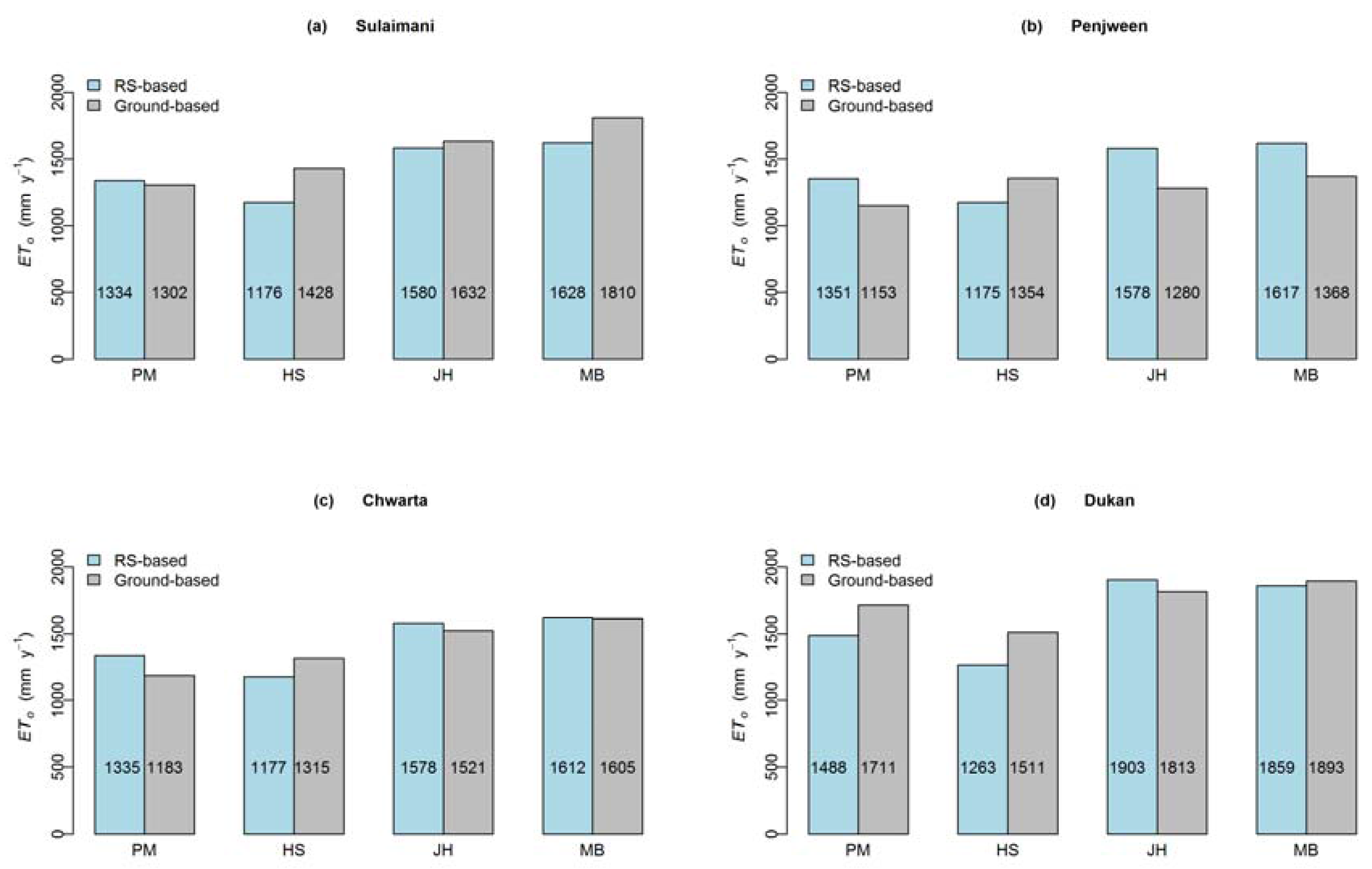
The calculated daily ETo-G and ETₒ-RS estimates are shown in Figure 4. In all cases, the black line shows ETo–G. For all stations, there is seasonal agreement between ETo-G and ETo–RS for all evapotranspiration methods. Estimated ETo-G is plotted against ETo-RS in Figure 5, along with the best-fit linear regression and the 1:1 line. Most of the points are scattered around the 1:1 line for the JH and MB methods which always have high R2 and regression gradients close to unity. However, there is considerable variability in the slope of the ground-derived versus RS-derived regression lines (0.7 to 0.89) and in R2 (0.64 to 0.9) when using the HS and PM methods—particularly for the Dukan and Sulaimani stations. These stations have relatively low elevations compared with the other two stations, with higher average temperatures (Table 1). Average annual ET0 values estimated using the ground and RS data for all methods from 2010 to 2014 are presented in Figure 6. The MB method yielded highest average annual values for both ETo-G and ETo-RS (1670 mm year−1 and 1677 mm year−1, respectively), while the HS method yielded the lowest annual value of ETo-RS (1198 mm year−1) and the PM method yielded lowest annual values of ETo-G (1337 mm year−1). The average annual values of ETo-RS were relatively similar to those of ETo-G, which reflects low bias and hence small cumulative errors.
Goodness-of-fit statistics are presented in Table 3. The MB method consistently performed better than other methods (in terms of the similarity of the ETo-G and ETₒ-RS data) for all stations and for all goodness-of-fit criteria, except for the bias at Sulaimani. The greatest differences were observed when the PM and HS methods are compared. The HS method consistently underestimated ground-based ET estimates when RS data were used as inputs (i.e., bias was always negative). Pearson correlation coefficients (r) between ETₒ-G and ETₒ-RS were generally high and always highly significant (p < 0.05) for all stations.
3.3. Cross-Comparison of the ETₒ Methods
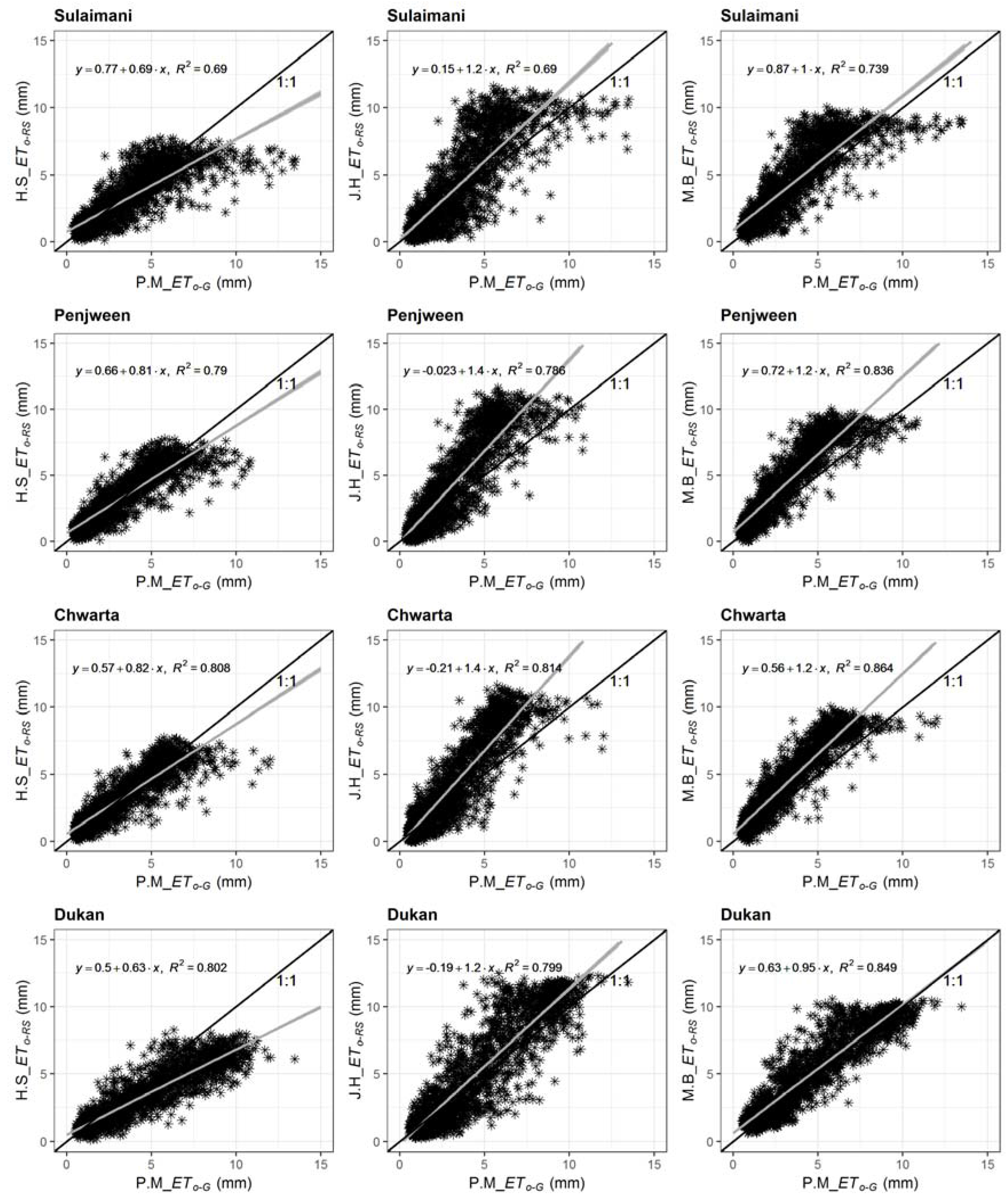
In Figure 7, different ETₒ-RS values calculated using the HS, JH, and MB methods are plotted against benchmark data (i.e., ETₒ-G PM) for all stations. This comparison is based on the assumption that the PM method is most reliable [49], and that the ground-based measurements at each station best represent the atmospheric drivers for evapotranspiration (i.e., the ground-based data will best-predict ETo using the PM method). There was considerable variation in model performance against the benchmark data for different stations. The JH and MB methods had regression slopes in the range between 0.95 and 1.4, with most slopes >1, indicating a slight tendency of these methods to overestimate the benchmark values. However, the slopes for the HS method ranged between 0.63 and 0.82, suggesting a tendency for the HS equation to under-predict ET when driven by RS data, particularly at the Dukan station Although the MB method yielded the best coefficient of determination for each station (0.74 < R2 < 0.86), this was not always the best method in terms of proximity to the 1:1 line. At the two stations with higher elevation (Penjween and Chwarta) the HS method was the best predictor. Table 4 summarises the results statistically. This confirms that the HS method tends to underestimate benchmark ET (−9 < bias% < −0.6) and that the other methods tend to overestimate it (bias ranged between 8.6 and 40%). At all stations the HS method had the lowest RMSE (1–1.3 mm day−1). Despite the fact that the JH and MB methods had correlation coefficients which were often better than for the HS method, they had much higher RMSE values (1.8–2.1 mm day−1).
4. Discussion
In this paper, reference evapotranspiration (ETₒ) was estimated based on four methods using ground-observed and RS-derived meteorological data (i.e., AIRS and reanalysis wind speed data from MERRA) at four stations in northeastern Iraq. For mean daily air temperature, AIRS and ground-based measurements were very similar for all sampled stations. The positive bias for increased with increasing station altitude. Similarly, for RH the relationship between AIRS and ground-based measurements was strong, albeit with a negative bias, for all stations. Despite the better spatial resolution of the MERRA data compared to AIRS data, we decided not to use the MERRA products because we wanted, explicitly, to focus on the value of the RS data and avoid reanalysis products as much as possible. Reanalysis data (which often integrate data from different sources) can be sensitive to observing system changes and there is often some uncertainty due to variations in both the models used and in the analysis techniques employed [31]. Unfortunately, we were not able to avoid using reanalysis products completely and MERRA wind speed data () was required because to date no RS wind speed data are available. The relationships for DS and were weak for all stations. The effect of differences between RS and ground-based meteorological variables on ETₒ rate will depend on the model sensitivity to the variable in question (i.e., if the model is sensitive to an input variable then predictions of ET will differ significantly if the RS estimate for that variable differs from the ground-based measurement; conversely, if the model is insensitive to the variable in question then ET will be relatively unaffected by errors in the RS estimates). Differences could be due to the different spatial reference frames employed, with meteorological stations recording point measurements and RS platforms observing spatially aggregated variables over large grid cells or pixels. As well as altering ET using empirical methods, differences in estimates will also affect other temperature-dependent values such as vapour pressure deficit and ∆.
There was generally reasonable agreement between ETₒ-RS and ETₒ-G for all the ETₒ methods evaluated, based on high R2 values and regression line slopes close to unity compared with the predictions driven by ground-based measurements. However, there was some variation in model performance for individual stations. Regressions between the bias in input variables (RS versus ground) and the bias in ETₒ estimates (calculated using RS versus the benchmark) for all methods are shown in Table S2. Strong and significant relationships were observed between the bias in sunshine duration and the bias in ETₒ in the case of the JH and MB methods (R2 > 0.95, p < 0.05) for all stations. This is not unexpected, given the dependence of these methods on solar radiation (and indirectly DS) suggesting high sensitivity. Other relationships were insignificant – even for the bias in ET from the HS method versus the bias in Ta, possibly because the HS method also depends on the theoretical radiation flux density at the top of the atmosphere. The bias in ETₒ-RS for the PM equation was most sensitive to DS and wind speed, reflecting the high importance of both radiative and aerodynamic terms in this method (by definition).
The PM model tended to predict lower ETₒ than when using ground-based data for the Dukan station, but higher ETₒ for the Sulaimani, Penjween and Charta stations. This is mainly due to the sensitivity of the PM method to meteorological input data (i.e., radiation, air temperature, humidity and wind speed [9]). Thus, the effects of disparities between ground-level measurements and RS estimates can be significant on ETₒ calculations especially in windy, warm and or dry conditions [9]. For instance, derived from RS overestimated ground-based measurements for the Penjween and Charta stations in the mountains (1284 and 1128 m ASL, respectively) but underestimated at Dukan, which is located at lower altitude (690 m ASL). These results agree with the results reported by Ferguson and Wood [50] which showed that the positive bias of near-surface air temperature from AIRS increased with increasing elevation. Similar to , DS and also contributed significantly to the deviation of RS and ground-driven ET using the PM method due to high bias and RMSE for the RS-estimates of these variables compared to ground-based measurements.
In the cross-comparison of the ETₒ methods (i.e., when the RS-driven models were compared with the benchmark data set), ETₒ-RS (HS) slightly underestimated ETₒ-G (PM: Table 4). This could be due to: (i) The absence of humidity terms in the HS method [32,51] in contrast to the PM method in which ETₒ is positively correlated with vapour pressure deficit. This is especially important in semi-arid environments were humidity deficits can be high (i.e., when low relative humidity results in a steep gradient in vapour pressure between the surface and the bulk atmosphere). (ii) The fact that temperature-based methods (HS) tend to underestimate ETₒ at high wind speeds of >3 m s−1 [49]. In the original PM method, wind speed is included via the aerodynamic resistance term (which is combined with the surface resistance, specific heat capacity and air density in the FAO version shown in Equation (6) via the constants 900 and 0.34). (iii) The fact that atmospheric transmissivity (the ratio of the global solar radiation at ground level to that received at the top of the atmosphere, [52,53]) in semi-arid area tends to differ from other areas due to lower atmospheric moisture content [52]. A number of other studies [54,55,56,57,58,59] have reported that the HS method can overestimate ETₒ in humid environments and under estimate it in semi-arid regions [47]. Although a slight negative bias was also observed here, the HS model yielded lower RMSE values overall compared with the other methods suggesting that it is a reasonable method for estimating ETₒ in semi-arid regions similar to our study area (even when driven by RS data). This result is in agreement with Lopez et al. [7], Tabari [47] and Tabari and Talaee [59] who concluded that the HS method can be successfully used in semi-arid areas.
The positive bias obtained from comparisons between ETₒ-RS calculated using the JH and MB methods and ETₒ-G PM is in accordance with both Jensen et al. [36] and Tabari et al. [32] who found that these models tend to overestimate ETo compared with the PM method, by as much as 30% and 60%, respectively. In our study the JH and MB methods overestimated the benchmark average annual ETₒ at all stations (Figure 6) by between 9% and 40%. Instead, the average annual ETₒ predicted by the HS method was similar to that estimated by the PM method for all stations (e.g., bias ranged between −0.6% and −9%).
This study did not take into account the effects of vegetation factors on the ET rate and, instead, focussed on climatic factors. ETₒ expresses the evaporation power of the atmosphere at a specific location and time of the year and does not consider land cover characteristics and soil factors [9]. If required, crop-specific ETp can be calculated from ETₒ using crop-specific resistance terms in the PM equation or, more generally, using crop coefficients [9] which account for differences in vegetation canopy characteristics such as leaf area index, canopy height and stomatal resistance. ETa can be calculated from ETp (or ETₒ) if soil moisture content can be estimated, often via a linear reduction in ETa:ETp between a threshold moisture content and the permanent wilting point [13].
5. Conclusions
Obtaining accurate estimates of ETₒ is essential for well-informed water management. However, in many parts of the world, the meteorological data required to estimate it are not available or are very scarce. Satellite remote sensing offers an alternative data source to ground stations, provided it can be shown to provide robust and reliable estimates of water fluxes. In this study, we assessed the validity of using daily RS-derived meteorological variables for estimating daily ETₒ compared with ETₒ from the same models driven by ground-based meteorological variables, for four stations in northeastern Iraq. The results were also compared with a benchmark model (PM) driven by ground-based meteorological observations. The good agreement (i.e., low RMSE and bias and high r) between AIRS and ground-based data, particularly near-surface air temperature, and the generally good performance of the ET models compared to the benchmark data set, suggest that AIRS data can be used as alternatives to conventional meteorological data to estimate daily ETₒ with reasonable accuracy. Considering the low density of ground-based stations and the paucity of climatological records in regions such as Iraq, this is encouraging for future hydrological studies and for better-informed water management. The application of the PM method is limited in many semi-arid regions of the world by lack of required weather observations. In such circumstances, simpler models are often used to estimate ETₒ. In this case, the RS-driven HS method produced better ETₒ estimates (compared to the PM equation as a benchmark) than the other models. It is recommended that the HS model is used where complete weather observation data are lacking. This method can be successfully employed using RS data to yield accurate and useful daily ETₒ estimates. This, in turn, is valuable for better policy making and planning in order to ensure efficient use of water resources, to improve irrigation management and for hydrological modelling. Some reanalysis data products already exist which attempt to estimate ETₒ using a combination of RS and ground-based data and numerical models (e.g., MERRA-2). Future work could usefully compare ETₒ estimates generated here with those predicted by MERRA-2.
Supplementary Materials
The following are available online at www.mdpi.com/2072-4292/9/8/779/s1. Figure S1: Plot of daily ETₒ estimates derived from ground-based measurements (ETₒ-G) and remote sensing data (ETₒ-RS) using PM method from 2010–2014 for Sulaimani, Penjween, Chwarta and Dukan stations. The black line presents the ETₒ-G. The blue line presents the ETₒ-RS when the PM model driven by constant-wind speed. The green line presents the ETₒ-RS when the PM model driven by MERRA-wind speed, Figure S2: Scatterplots of estimated daily reference evapotranspiration using ground-based measurements using PM method (ETₒ-G) versus estimated reference evapotranspiration using remote sensing data (ETₒ-RS) using PM method when the PM was driven by with MERAA-wind speed and constant-wind speed at four different stations (Sulaimani, Penjween, Chwarta, and Dukan). The solid black line indicates the 1:1 relationship. The grey line shows the best-fit regression with 95% confidence interval (equations and R2 also shown), Table S1: Statistical summary of comparisons between estimated daily reference evapotranspiration using ground-based measurements (ETₒ-G) and remote sensing data (ETₒ-RS) with MERRA-wind speed and constant-wind speed data for PM methods at four different stations (Sulaimani, Penjween, Chwarta, and Dukan) over the study period 2010-2014. * means significant at p < 0.05, Table S2: Statistical summary of (BIAS%) between daily ground-measured and remotely-sensed values of , RH%, and and BIAS% summary of estimated daily reference evapotranspiration using remote sensing data (ETₒ-RS) for four different methods against the benchmark data set (PM method using ground-based measurements: ETₒ-G: PM) for four different stations (Sulaimani, Penjween, Chwarta, and Dukan) over the study period 2010–2014. * means significant at p < 0.05, Table S3: Summary of annual ETₒ-G and ETₒ-RS (with MERRA-wind speed and constant-wind speed data) for PM method at four different stations (Sulaimani, Penjween, Chwarta, and Dukan) over the study period 2010–2014.
Acknowledgments
This research was funded via a scholarship from The Higher Committee for Education Development in Iraq (HCED) with support from the NERC National Centre for Earth Observation. We are grateful to the Directorate of Meteorology in Sulaimanyiah for providing meteorological data. HB was supported by a Royal Society Wolfson Research Merit Award (2011/R3) and the NERC National Centre for Earth Observation (NCEO) and MW benefitted from Study Leave granted by the University of Leicester.
Author Contributions
This paper is the result of research conducted by Peshawa Najmaddin (PN) as part of his PhD studies at the University of Leicester. Mick Whelan (MW) and Heiko Balzter (HB) jointly supervised this project. HB provided guidance on the analysis of the remote sensing data. The manuscript was prepared by PN with suggestions and corrections from MW and HB. All authors have seen and approved the final article.
Conflicts of Interest
The authors declare no conflict of interest. The founding sponsors had no role in the design of the study; in the collection, analyses, or interpretation of data; in the writing of the manuscript, and in the decision to publish the results.
References
- Zhao, L.; Xia, J.; Xu, C.-Y.; Wang, Z.; Sobkowiak, L.; Long, C. Evapotranspiration estimation methods in hydrological models. J. Geogr. Sci. 2013, 23, 359–369. [Google Scholar] [CrossRef]
- Nikam, B.R.; Kumar, P.; Garg, V.; Thakur, P.K.; Aggarwal, S.P. Comparative evaluation of different potential evapotranspiration estimation approaches. Int. J. Res. Eng. Technol. 2014, 3, 543–552. [Google Scholar]
- Pilgrim, D.H.; Chapman, T.G.; Doran, D.G. Problems of rainfall-runoff modelling in arid and semiarid regions. Hydrol. Sci. J. 1988, 33, 379–400. [Google Scholar] [CrossRef]
- Chahine, M. The hydrological cycle and its influence on climate. Nat. Publ. Group 1992, 359, 373–379. [Google Scholar] [CrossRef]
- Shaw, E.M. Hydrology in Practice; Chapman & Hall London: New York, NY, USA, 1994. [Google Scholar]
- Strugnell, N.; Lucht, W.; Schaaf, C. A global albedo data set derived from AVHRR data for use in climate simulations. Geophys. Res. Lett. 2001, 28, 191–194. [Google Scholar] [CrossRef]
- López-Urrea, R.; de Santa Olalla, F.M.; Fabeiro, C.; Moratalla, A. Testing evapotranspiration equations using lysimeter observations in a semiarid climate. Agric. Water Manag. 2006, 85, 15–26. [Google Scholar] [CrossRef]
- Beaumont, P.; Blake, G.; Wagstaff, J.M. The Middle East: A Geographical Study, 2nd ed.; Routledge: Oxford, UK, 2016. [Google Scholar]
- Allen, R.G.; Pereira, L.S.; Raes, D.; Smith, M. Crop Evapotranspiration-Guidelines for Computing Crop Water Requirements-FAO Irrigation and Drainage Paper 56; FAO: Rome, Italy, 1998; pp. 1–15. [Google Scholar]
- Tabari, H.; Aeini, A.; Talaee, P.H.; Some’e, B.S. Spatial distribution and temporal variation of reference evapotranspiration in arid and semi-arid regions of Iran. Hydrol. Process. 2012, 26, 500–512. [Google Scholar] [CrossRef]
- Herath, I.K.; Ye, X.; Wang, J.; Bouraima, A.-K. Spatial and temporal variability of reference evapotranspiration and influenced meteorological factors in the Jialing River Basin, China. Theor. Appl. Climatol. 2017, 129, 1–12. [Google Scholar]
- Alemayehu, T.; van Griensven, A.; Senay, G.B.; Bauwens, W. Evapotranspiration Mapping in a Heterogeneous Landscape Using Remote Sensing and Global Weather Datasets: Application to the Mara Basin, East Africa. Remote Sens. 2017, 9, 390. [Google Scholar] [CrossRef]
- Najmaddin, P.M.; Whelan, M.J.; Balzter, H. Application of Satellite-Based Precipitation Estimates to Rainfall-Runoff Modelling in a Data-Scarce Semi-Arid Catchment. Climate 2017, 5, 32. [Google Scholar] [CrossRef]
- Wilby, R.L.; Yu, D. Rainfall and temperature estimation for a data sparse region. Hydrol. Earth Syst. Sci. 2013, 17, 3937–3955. [Google Scholar] [CrossRef]
- Lee, Y.R.; Yoo, J.M.; Jeong, M.J.; Won, Y.I.; Hearty, T.; Shin, D.B. Comparison between MODIS and AIRS/AMSU satellite-derived surface skin temperatures. Atmos. Meas. Tech. 2013, 6, 445–455. [Google Scholar] [CrossRef]
- AIRS Science Team/Joao Texeira. Aqua AIRS Level 3 Daily Standard Physical Retrieval (AIRS + AMSU), Version 006; NASA Goddard Earth Science Data and Information Services Center (GES DISC): Greenbelt, MD, USA, 2013. Available online: https://disc.gsfc.nasa.gov/datasets/AIRX3STD_006/summary (accessed on 18 April 2016).
- Meier, D.C.; Fiorino, S.T. Application of Satellite- and NWP-Derived Wind Profiles to Military Airdrop Operations. J. Appl. Meteorol. Climatol. 2016, 55, 2197–2209. [Google Scholar] [CrossRef]
- Zhang, Y.Q.; Chiew, F.H.S.; Zhang, L.; Leuning, R.; Cleugh, H.A. Estimating catchment evaporation and runoff using MODIS leaf area index and the Penman-Monteith equation. Water Resour. Res. 2008, 44, 1–15. [Google Scholar] [CrossRef]
- Mu, Q.; Jones, L.A.; Kimball, J.S.; McDonald, K.C.; Running, S.W. Satellite assessment of land surface evapotranspiration for the pan-Arctic domain. Water Resour. Res. 2009, 45. [Google Scholar] [CrossRef]
- Rahimi, S.; Gholami Sefidkouhi, M.A.; Raeini-Sarjaz, M.; Valipour, M. Estimation of actual evapotranspiration by using MODIS images (a case study: Tajan catchment). Arch. Agron. Soil Sci. 2014, 61, 695–709. [Google Scholar] [CrossRef]
- Peng, J.; Loew, A.; Chen, X.; Ma, Y.; Su, Z. Comparison of satellite-based evapotranspiration estimates over the Tibetan Plateau. Hydrol. Earth Syst. Sci. 2016, 20, 3167–3182. [Google Scholar] [CrossRef]
- Mu, Q.; Zhao, M.; Running, S.W. Brief Introduction to MODIS Evapotranspiration Data Set (MOD16); University of Montana: Missoula, MT, USA, 2014; pp. 1–4. [Google Scholar]
- Global Modeling and Assimilation Office (GMAO). MERRA-2 tavgM_2d_flx_Nx: 2d, Monthly Mean, Time-Averaged, Single-Level, Assimilation, Surface Flux Diagnostics V5.12.4; Goddard Earth Sciences Data and Information Services Center (GES DISC): Greenbelt, MD, USA, 2015. [CrossRef]
- McNally, A. FLDAS Noah Land Surface Model L4 daily 0.1 × 0.1 Degree for Southern Africa (GDAS and RFE2) V001; NASA/GSFC/HSL: Greenbelt, MD, USA, 2016. Available online: https://disc.gsfc.nasa.gov/datacollection/FLDAS_NOAH01_A_SA_D_001.html (accessed on 25 January 2017).
- Jasinski, M. NCA-LDAS Noah-3.3 Land Surface Model L4 Daily 0.125 × 0.125 Degree V001; NASA/GSFC/HSL: Greenbelt, MD, USA, 2016. Available online: https://disc.sci.gsfc.nasa.gov/uui/datasets/NCALDAS_NOAH0125_D_001/summary (accessed on 24 January 2017).
- Qader, S.H.; Dash, J.; Atkinson, P.M.; Galiano, V.R. Classification of Vegetation Type in Iraq Using Satellite-Based Phenological Parameters. IEEE J. 2016, 43, 1–23. [Google Scholar] [CrossRef]
- Food and Agriculture Organization (FAO). Country Pasture/forage Resource Profiles. Rome, Italy, 2016. Available online: http://www.fao.org/geonetwork/srv/en/main.home?uuid=ba4526fd-cdbf-4028-a1bd-5a559c4bff38 (accessed on 9 January 2016).
- Zaitchik, B.F.; Evans, J.P.; Smith, R.B. Regional Impact of an Elevated Heat Source: The Zagros Plateau of Iran. J. Clim. 2007, 20, 4133–4146. [Google Scholar] [CrossRef]
- R Core Team. R: A Language and Environment for Statistical Computing; R Foundation for Statistical Computing: Vienna, Austria, 2014. [Google Scholar]
- McKinley, S.; Levine, M. Cubic spline interpolation. Coll. Redw. 1998, 45, 1049–1060. [Google Scholar]
- Rienecker, M.M.; Suarez, M.J.; Gelaro, R.; Todling, R.; Bacmeister, J.; Liu, E.; Bosilovich, M.G.; Schubert, S.D.; Takacs, L.; Kim, G.-K.; et al. MERRA: NASA’s Modern-Era Retrospective Analysis for Research and Applications. J. Clim. 2011, 24, 3624–3648. [Google Scholar] [CrossRef]
- Tabari, H.; Grismer, M.E.; Trajkovic, S. Comparative analysis of 31 reference evapotranspiration methods under humid conditions. Irrig. Sci. 2011, 31, 107–117. [Google Scholar] [CrossRef]
- McMahon, T.A.; Peel, M.C.; Lowe, L.; Srikanthan, R.; McVicar, T.R. Estimating actual, potential, reference crop and pan evaporation using standard meteorological data: A pragmatic synthesis. Hydrol. Earth Syst. Sci. 2013, 17, 1331–1363. [Google Scholar] [CrossRef]
- Brutsaert, W. Evaporation into the Atmosphere: Theory, History and Applications; Springer Science & Business Media: Berlin/Heidiberg, Germany, 1982; Volume 1. [Google Scholar]
- Poyen, E.F.B.; Ghosh, A.K. Review on Different Evapotranspiration Empirical Equations. IJAEMS Open Access Int. J. Infogain Publ. 2016, 2, 17–24. [Google Scholar]
- Jensen, M.E.; Burman, R.D.; Allen, R.G. Evapotranspiration and Irrigation Water Requirements; ASCE: New York, NY, USA, 1990; p. 360. [Google Scholar]
- Thornthwaite, C.W. An approach toward a rational classification of climate. Geogr. Rev. 1948, 38, 55–94. [Google Scholar] [CrossRef]
- Hargreaves, G.H.; Samani, Z.A. Reference crop evapotranspiration from ambient air temperature. In Proceedings of the Winter Meeting of the American Society of Agricultural Engineers, Chicago, IL, USA, 17 December 1985. paper no. 85–2517. [Google Scholar]
- Jensen, M.E.; Haise, H.R. Estimating evapotranspiration from solar radiation. In Proceedings of the American Society of Civil Engineers. J. Irrig. Drain. Div. 1963, 89, 15–41. [Google Scholar]
- McGuinness, J.L.; Bordne, E.F. A comparison of lysimeter-derived potential evapotranspiration with computed values. In Technical Bulletin 1452, Agricultural Research Service; US Department of Agriculture: Washington, DC, USA, 1972. [Google Scholar]
- Priestley, C.; Taylor, R. On the assessment of surface heat flux and evaporation using large-scale parameters. Mon. Weather Rev. 1972, 100, 81–92. [Google Scholar] [CrossRef]
- Gong, L.; Xu, C.-Y.; Chen, D.; Halldin, S.; Chen, Y.D. Sensitivity of the Penman–Monteith reference evapotranspiration to key climatic variables in the Changjiang (Yangtze River) basin. J. Hydrol. 2006, 329, 620–629. [Google Scholar] [CrossRef]
- Pandey, P.K.; Dabral, P.P.; Pandey, V. Evaluation of reference evapotranspiration methods for the northeastern region of India. Int. Soil Water Conserv. Res. 2016, 4, 52–63. [Google Scholar] [CrossRef]
- Sabziparvar, A.-A.; Tabari, H.; Aeini, A.; Ghafouri, M. Evaluation of Class A Pan Coefficient Models for Estimation of Reference Crop Evapotranspiration in Cold Semi-Arid and Warm Arid Climates. Water Resour. Manag. 2009, 24, 909–920. [Google Scholar] [CrossRef]
- Tabari, H.; Kisi, O.; Ezani, A.; Hosseinzadeh Talaee, P. SVM, ANFIS, regression and climate based models for reference evapotranspiration modeling using limited climatic data in a semi-arid highland environment. J. Hydrol. 2012, 444–445, 78–89. [Google Scholar] [CrossRef]
- WeiB, M.; Menzel, L. A global comparison of four potential evapotranspiration equations and their relevance to stream flow modelling in semi-arid environments. Adv. Geosci. 2008, 18, 15–23. [Google Scholar]
- Tabari, H. Evaluation of Reference Crop Evapotranspiration Equations in Various Climates. Water Resour. Manag. 2009, 24, 2311–2337. [Google Scholar] [CrossRef]
- Oudin, L.; Hervieu, F.; Michel, C.; Perrin, C.; Andréassian, V.; Anctil, F.; Loumagne, C. Which potential evapotranspiration input for a lumped rainfall–runoff model? J. Hydrol. 2005, 303, 290–306. [Google Scholar] [CrossRef]
- Allen, R.; Smith, M.; Pereira, L.; Raes, D.; Wright, J. Revised FAO Procedures for Calculating Evapotranspiration–Irrigation and Drainage Paper No. 56 with Testing in Idaho. Bridges 2000, 1–10. [Google Scholar] [CrossRef]
- Ferguson, C.R.; Wood, E.F. An Evaluation of Satellite Remote Sensing Data Products for Land Surface Hydrology: Atmospheric Infrared Sounder. J. Hydrometeorol. 2010, 11, 1234–1262. [Google Scholar] [CrossRef]
- Temesgen, B.; Eching, S.; Davidoff, B.; Frame, K. Comparison of some reference evapotranspiration equations for California. J. Irrig. Drain. Eng. 2005, 131, 73–84. [Google Scholar] [CrossRef]
- Bo, H.; Yue-Si, W.; Guang-Ren, L. Properties of Solar Radiation over Chinese Arid and Semi-Arid Areas. Atmos. Ocean. Sci. Lett. 2009, 2, 183–187. [Google Scholar] [CrossRef]
- Baigorria, G.A.; Villegas, E.B.; Trebejo, I.; Carlos, J.F.; Quiroz, R. Atmospheric transmissivity: Distribution and empirical estimation around the central Andes. Int. J. Climatol. 2004, 24, 1121–1136. [Google Scholar] [CrossRef]
- Jensen, D.; Hargreaves, G.; Temesgen, B.; Allen, R. Computation of ETo under nonideal conditions. J. Irrig. Drain. Eng. 1997, 123, 394–400. [Google Scholar] [CrossRef]
- Kashyap, P.; Panda, R. Evaluation of evapotranspiration estimation methods and development of crop-coefficients for potato crop in a sub-humid region. Agric. Water Manag. 2001, 50, 9–25. [Google Scholar] [CrossRef]
- Yoder, R.; Odhiambo, L.; Wright, W. Evaluation of methods for estimating daily reference crop evapotranspiration at a site in the humid southeast United States. Appl. Eng. Agric. 2005, 21, 197–202. [Google Scholar] [CrossRef]
- Trajkovic, S. Hargreaves versus Penman-Monteith under humid conditions. J. Irrig. Drain. Eng. 2007, 133, 38–42. [Google Scholar] [CrossRef]
- Landeras, G.; Ortiz-Barredo, A.; López, J.J. Comparison of artificial neural network models and empirical and semi-empirical equations for daily reference evapotranspiration estimation in the Basque Country (Northern Spain). Agric. Water Manag. 2008, 95, 553–565. [Google Scholar] [CrossRef]
- Tabari, H.; Talaee, P.H. Local Calibration of the Hargreaves and Priestley-Taylor Equations for Estimating Reference Evapotranspiration in Arid and Cold Climates of Iran Based on the Penman-Monteith Model. J. Hydrol. Eng. 2011, 16, 837–845. [Google Scholar] [CrossRef]
Figure 1.
(a) Elevation in the study area derived from the Shuttle Radar Topography Mission (SRTM) digital elevation model (DEM) (https://earthexplorer.usgs.gov/). (b) Regional location of the study area.
Figure 1.
(a) Elevation in the study area derived from the Shuttle Radar Topography Mission (SRTM) digital elevation model (DEM) (https://earthexplorer.usgs.gov/). (b) Regional location of the study area.
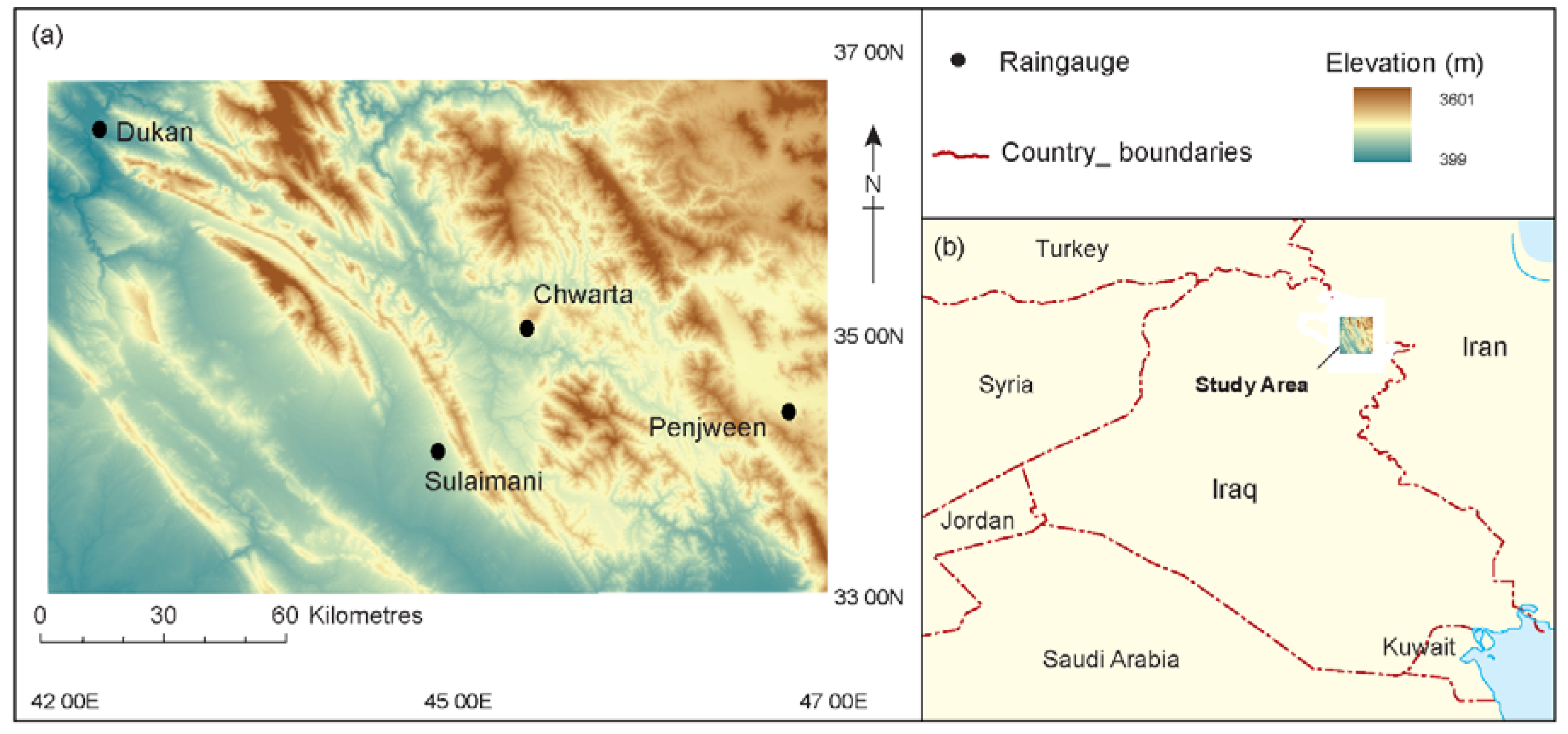
Figure 2.
Mean monthly rainfall (spatially averaged over Thiessen polygons), temperature and relative humidity (RH) in the study area 2010–2014 (Sulaimani Meteorological Office, 2015).
Figure 2.
Mean monthly rainfall (spatially averaged over Thiessen polygons), temperature and relative humidity (RH) in the study area 2010–2014 (Sulaimani Meteorological Office, 2015).
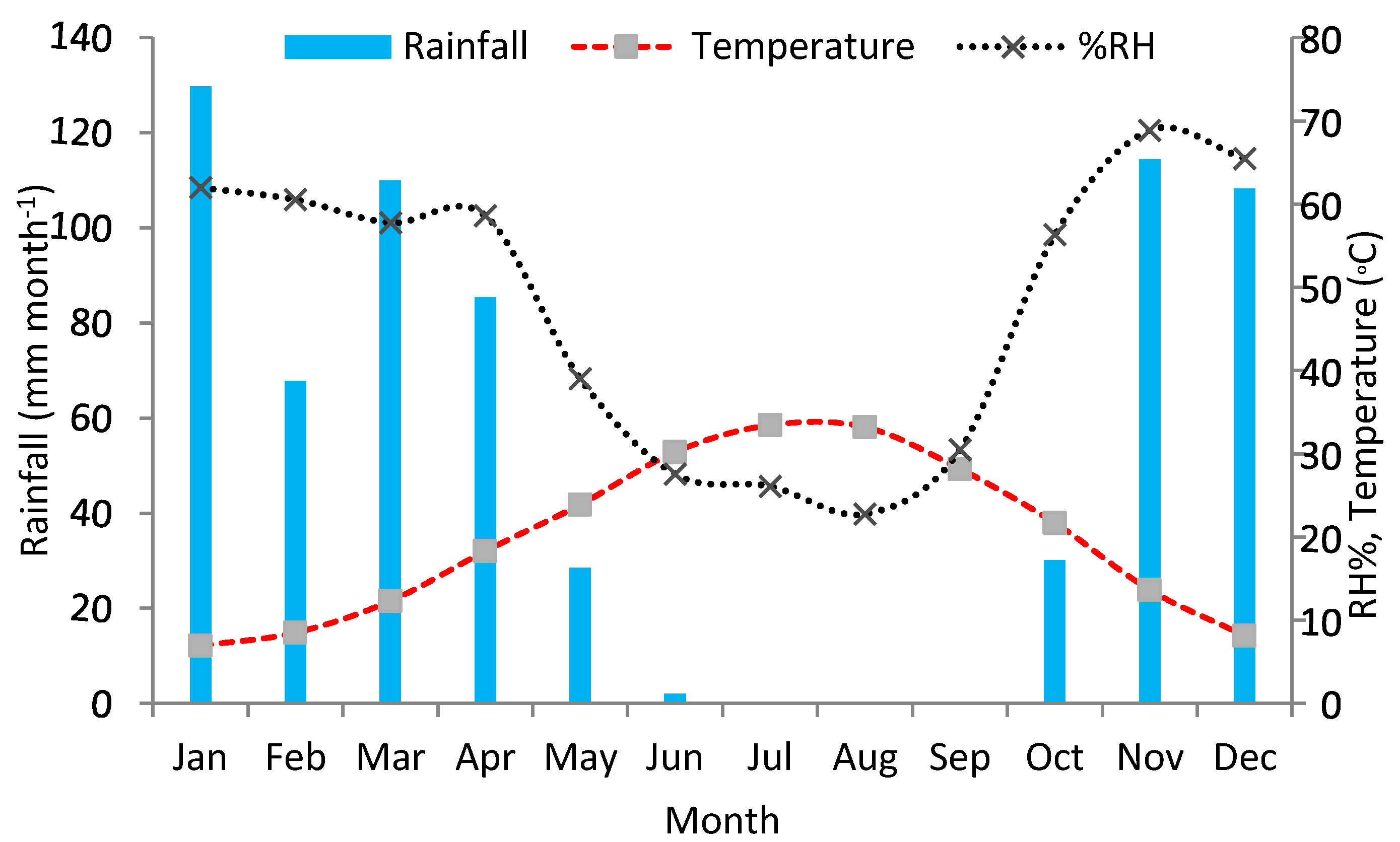
Figure 3.
Scatterplots of daily , RH %, and measured at ground-based stations (x-axes) compared with those derived from remote sensing (y-axes) for four different stations. The solid black line indicates the 1:1 relationship. The grey line shows the best-fit regression with 95% confidence interval.
Figure 3.
Scatterplots of daily , RH %, and measured at ground-based stations (x-axes) compared with those derived from remote sensing (y-axes) for four different stations. The solid black line indicates the 1:1 relationship. The grey line shows the best-fit regression with 95% confidence interval.
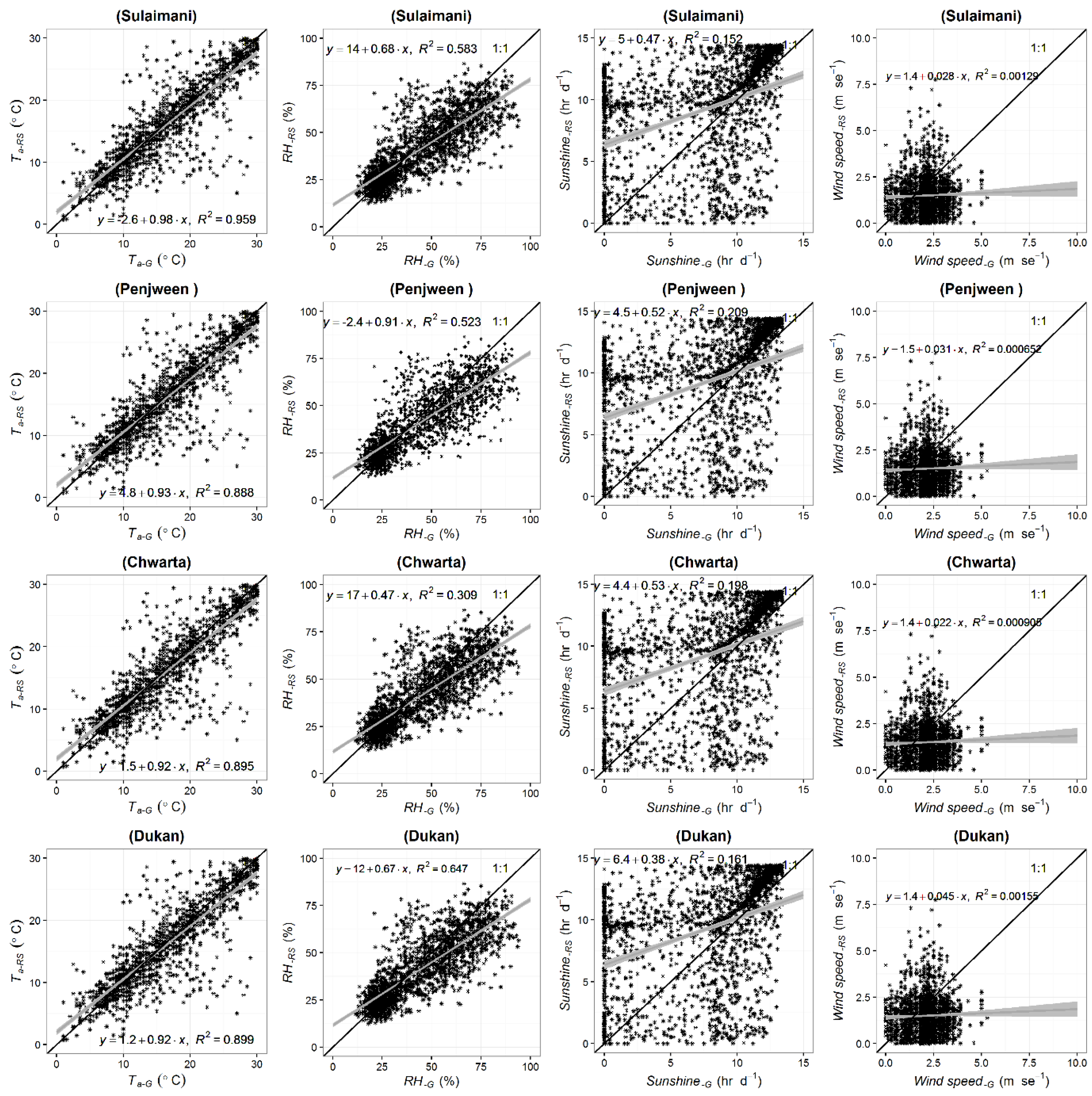
Figure 4.
Plot of daily ETₒ estimates derived from ground-based measurements (ETₒ-G) and remote sensing data (ETₒ-RS) using four methods from 2010–2014 for Sulaimani, Penjween, Chwarta and Dukan stations. The black line presents the ETₒ-G.
Figure 4.
Plot of daily ETₒ estimates derived from ground-based measurements (ETₒ-G) and remote sensing data (ETₒ-RS) using four methods from 2010–2014 for Sulaimani, Penjween, Chwarta and Dukan stations. The black line presents the ETₒ-G.
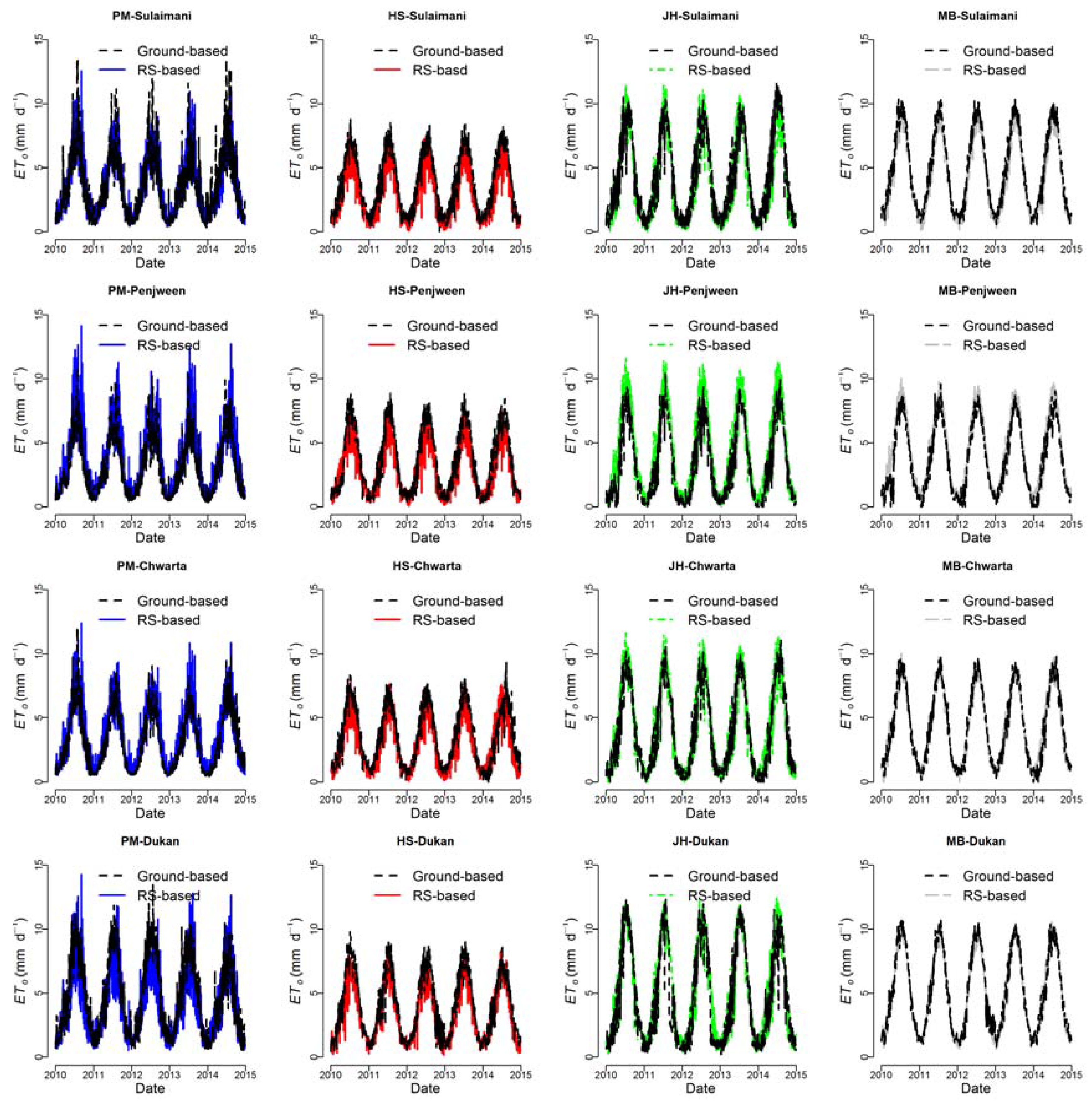
Figure 5.
Scatterplots of estimated daily reference evapotranspiration using ground-based measurements (ETₒ-G) versus estimated reference evapotranspiration using remote sensing data (ETₒ-RS) applying four different methods at four different stations (Sulaimani, Penjween, Chwarta, and Dukan). The solid black line indicates the 1:1 relationship. The grey line shows the best-fit regression with 95% confidence interval (equations and R2 also shown).
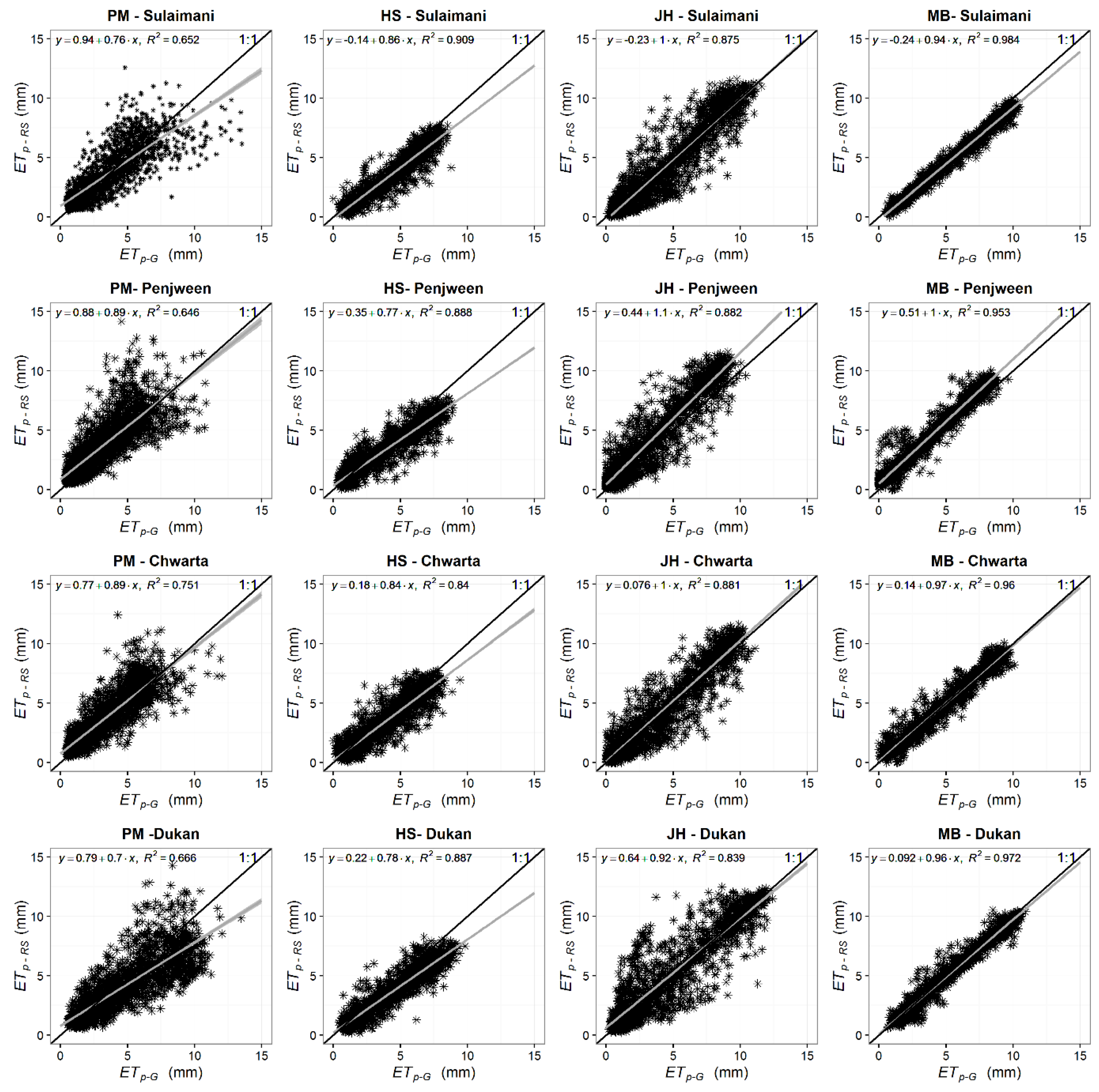
Figure 6.
Average annual ETₒ estimates derived from ground-based measurements (ETₒ-G) and remote sensing data (ETₒ-RS) using four methods from 2010–2014 for Sulaimani, Penjween, Chwarta and Dukan stations.
Figure 6.
Average annual ETₒ estimates derived from ground-based measurements (ETₒ-G) and remote sensing data (ETₒ-RS) using four methods from 2010–2014 for Sulaimani, Penjween, Chwarta and Dukan stations.

Figure 7.
Scatterplots of estimated daily reference evapotranspiration using remote sensing data (ETₒ-RS) for the HS, JH and MB methods against estimated reference evapotranspiration generated using ground-based measurements (ETₒ-G) with the PM method (the benchmark model) for four different stations (Sulaimani, Penjween, Chwarta and Dukan). The solid black line indicates the 1:1 relationship. The grey line shows the best-fit regression with 95% confidence interval (equations and R2 also shown).


Table 1.
Elevation, mean daily temperature, relative humidity and average annual rainfall for the four stations located in the study area from 2010 to 2014 (Sulaimani Meteorological Office, 2015).
Table 1.
Elevation, mean daily temperature, relative humidity and average annual rainfall for the four stations located in the study area from 2010 to 2014 (Sulaimani Meteorological Office, 2015).
| Stations | Elevation (m) | Mean Daily Temperature (°C) | Relative Humidity (%) | Rainfall (mm year−1) |
|---|---|---|---|---|
| Dukan | 650 | 23.1 | 44.2 | 586.3 |
| Sulaimani | 885 | 20.1 | 45.2 | 646.7 |
| Chwarta | 1128 | 19.6 | 46.1 | 693.2 |
| Penjween | 1300 | 14 | 57.1 | 951 |
Table 2.
Statistical summary of the relationship between daily ground-measured and remotely-sensed values of , RH %, and for four different stations during the study period (2010–2014).
Table 2.
Statistical summary of the relationship between daily ground-measured and remotely-sensed values of , RH %, and for four different stations during the study period (2010–2014).
| Station | Variable | RMSE | BIAS (%) | R |
|---|---|---|---|---|
| Sulaimani | 3.5 | −14.2 | 0.97 | |
| RH % | 12.7 | −0.6 | 0.76 | |
| 4.5 | 16.1 | 0.38 | ||
| 1.4 | 27.8 | 0.03 | ||
| Penjween | 5.1 | 28.4 | 0.94 | |
| RH % | 13.8 | −13.4 | 0.72 | |
| 4.3 | 10.2 | 0.45 | ||
| 1.7 | 34.8 | 0.02 | ||
| Chwarta | 3.3 | −0.1 | 0.94 | |
| RH % | 24 | −26 | 0.55 | |
| 4.2 | 9.1 | 0.44 | ||
| 1.5 | 24.5 | 0.03 | ||
| Dukan | 3.2 | −2.8 | 0.95 | |
| RH % | 12.5 | −7.3 | 0.80 | |
| 5.1 | 21.8 | 0.40 | ||
| 1.4 | −47.7 | 0.03 |
Table 3.
Statistical summary of comparisons between estimated daily reference evapotranspiration using ground-based measurements (ETₒ-G) and remote sensing data (ETₒ-RS) for four different methods at four different stations (Sulaimani, Penjween, Chwarta, and Dukan) over the study period 2010–2014.
Table 3.
Statistical summary of comparisons between estimated daily reference evapotranspiration using ground-based measurements (ETₒ-G) and remote sensing data (ETₒ-RS) for four different methods at four different stations (Sulaimani, Penjween, Chwarta, and Dukan) over the study period 2010–2014.
| Station | Methods | RMSE (mm day−1) | BIAS (%) | R |
|---|---|---|---|---|
| Sulaimani | PM | 0.99 | 2.5 | 0.80 |
| HS | 1.26 | −17 | 0.95 | |
| JH | 0.82 | −3.2 | 0.93 | |
| MB | 0.65 | −10.5 | 0.99 | |
| Penjween | PM | 1.59 | 17.7 | 0.81 |
| HS | 1 | −13 | 0.94 | |
| JH | 1.46 | 23.2 | 0.93 | |
| MB | 0.92 | 18.2 | 0.97 | |
| Chwarta | PM | 1.26 | 12.8 | 0.86 |
| HS | 0.95 | −10 | 0.92 | |
| JH | 1.19 | 3.7 | 0.93 | |
| MB | 0.57 | 0.3 | 0.97 | |
| Dukan | PM | 1.7 | −13 | 0.81 |
| HS | 1.1 | −19.9 | 0.94 | |
| JH | 1.56 | 5.1 | 0.91 | |
| MB | 0.52 | −1.8 | 0.98 |
Table 4.
Statistical bias, RMSE and Pearson Product Moment Correlation coefficient (r) for ETₒ-RS values against the benchmark data set ETₒ-G (PM) for the different stations over the study period 2010–2014.
Table 4.
Statistical bias, RMSE and Pearson Product Moment Correlation coefficient (r) for ETₒ-RS values against the benchmark data set ETₒ-G (PM) for the different stations over the study period 2010–2014.
| Station | Methods | RMSE (mm day−1) | BIAS (%) | R |
|---|---|---|---|---|
| Sulaimani | HS | 1.3 | −9 | 0.83 |
| JH | 2.1 | 21.4 | 0.83 | |
| MB | 1.6 | 24.5 | 0.85 | |
| Penjween | HS | 1 | −1.9 | 0.88 |
| JH | 2.1 | 37 | 0.88 | |
| MB | 1.7 | 40 | 0.91 | |
| Chwarta | HS | 0.98 | −0.6 | 0.89 |
| JH | 2 | 33.3 | 0.90 | |
| MB | 1.6 | 37 | 0.92 | |
| Dukan | HS | 1.2 | −2.6 | 0.89 |
| JH | 1.8 | 11.2 | 0.89 | |
| MB | 1.81 | 8.6 | 0.92 |
© 2017 by the authors. Licensee MDPI, Basel, Switzerland. This article is an open access article distributed under the terms and conditions of the Creative Commons Attribution (CC BY) license (http://creativecommons.org/licenses/by/4.0/).
Share and Cite
MDPI and ACS Style
Najmaddin, P.M.; Whelan, M.J.; Balzter, H. Estimating Daily Reference Evapotranspiration in a Semi-Arid Region Using Remote Sensing Data. Remote Sens. 2017, 9, 779. https://doi.org/10.3390/rs9080779
AMA Style
Najmaddin PM, Whelan MJ, Balzter H. Estimating Daily Reference Evapotranspiration in a Semi-Arid Region Using Remote Sensing Data. Remote Sensing. 2017; 9(8):779. https://doi.org/10.3390/rs9080779
Chicago/Turabian StyleNajmaddin, Peshawa M., Mick J. Whelan, and Heiko Balzter. 2017. "Estimating Daily Reference Evapotranspiration in a Semi-Arid Region Using Remote Sensing Data" Remote Sensing 9, no. 8: 779. https://doi.org/10.3390/rs9080779
Note that from the first issue of 2016, this journal uses article numbers instead of page numbers. See further details here.