Elevation Extraction and Deformation Monitoring by Multitemporal InSAR of Lupu Bridge in Shanghai

Abstract

Monitoring, assessing, and understanding the structural health of large infrastructures, such as buildings, bridges, dams, tunnels, and highways, is important for urban development and management, as the gradual deterioration of such structures may result in catastrophic structural failure leading to high personal and economic losses. With a higher spatial resolution and a shorter revisit period, interferometric synthetic aperture radar (InSAR) plays an increasing role in the deformation monitoring and height extraction of structures. As a focal point of the InSAR data processing chain, phase unwrapping has a direct impact on the accuracy of the results. In complex urban areas, large elevation differences between the top and bottom parts of a large structure combined with a long interferometric baseline can result in a serious phase-wrapping problem. Here, with no accurate digital surface model (DSM) available, we handle the large phase gradients of arcs in multitemporal InSAR processing using a long–short baseline iteration method. Specifically, groups of interferometric pairs with short baselines are processed to obtain the rough initial elevation estimations of the persistent scatterers (PSs). The baseline threshold is then loosened in subsequent iterations to improve the accuracy of the elevation estimates step by step. The LLL lattice reduction algorithm (by Lenstra, Lenstra, and Lovász) is applied in the InSAR phase unwrapping process to rapidly reduce the search radius, compress the search space, and improve the success rate in resolving the phase ambiguities. Once the elevations of the selected PSs are determined, they are used in the following two-dimensional phase regression involving both elevations and deformations. A case study of Lupu Bridge in Shanghai is carried out for the algorithm’s verification. The estimated PS elevations agree well (within 1 m) with the official Lupu Bridge model data, while the PS deformation time series confirms that the bridge exhibits some symmetric progressive deformation, at 4–7 mm per year on both arches and 4–9 mm per year on the bridge deck during the SAR image acquisition period.

1. Introduction

Space borne interferometric synthetic aperture radar (InSAR) technology makes use of interferometric image pairs of the same ground area obtained from repeating satellite orbits. Interferometric phases from the image pairs can be used to determine elevation and deformation in the radar line of sight (LOS) direction [1,2]. With a high spatial resolution and a short revisit period, InSAR can be used for large-scale deformation monitoring and elevation extraction and has great application potential in areas such as health monitoring of large structures [3,4,5,6,7,8,9]. As interferograms are produced by the complex multiplication of coherent synthetic aperture radar (SAR) images, phase unwrapping is required to determine the number of whole phase cycles for arcs of interferometric phase observables in multitemporal InSAR data processing. Phase unwrapping is a core of InSAR technology. Many methods have been developed for phase unwrapping, including, e.g., the two-dimensional branch-cut method [10], the quality map guidance algorithm [11], the region-growing algorithm [12], the network flow method [13,14], three-dimensional phase unwrapping [15], and some others [16,17,18]. Each of the methods has its advantages and limitations.

In mathematics, phase unwrapping can be seen as the closest lattice vector problem; the lattice reduction algorithm is designed to find the shortest vector in a two-dimensional grid. In 1982, Lenstra, Lenstra, and Lovász proposed the LLL lattice reduction algorithm [19] to extend the search space to an n-dimensional space. Since the lattice reduction method can rapidly reduce the search radius, compress the search space, and improve the successful rate of ambiguity resolution, it has been widely used in integer programming [20], cryptography [21,22], number theory [23], and other fields. For example, it was applied by Liu to resolve Global Navigation Satellite System (GNSS) phase ambiguity [24]. We propose in this paper to use the LLL lattice reduction algorithm for InSAR phase unwrapping.

The classical permanent scatterer interferometry (PSI) model estimates linear deformation rate and elevation error simultaneously [1]. However, because the interferometric fringes are relatively dense in the case of a long baseline, a non-continuous steep slope phase corresponding to a large elevation gap may bring various challenges to a permanent scatterer (PS) arc’s solution. For example, the mean/sigma ratio of an arc may exceed the threshold value, so that some PSs may be eliminated. The obtained ambiguity may not be accurate, or the phase may be no longer continuous. Long-baseline interferometric pairs correspond to a smaller elevation ambiguity (namely, more accurate elevation); however, a long baseline also increases the difficulty of phase unwrapping. Conversely, short-baseline interferometric pairs correspond to a large elevation ambiguity (namely, less accurate elevation), but the interferometric fringes are relatively smooth and much easier to unwrap. In view of this, this paper makes use of the long–short baseline iteration method [25,26,27,28] for multitemporal InSAR data processing, which first selects short baseline interferometric pairs for a one-dimensional elevation solution, and then gradually enlarges the spatial baseline threshold and reduces the phase gradient with the elevation components calculated from the previous iteration. Once the elevations of the selected PSs are obtained with suitable accuracy, they are used in the following two-dimensional phase regression involving both the elevations and deformations. Finally, the linear and seasonal deformations are extracted from the multitemporal InSAR time series.

The paper demonstrates a method suitable for the high-phase-gradient phase unwrapping problem with no digital surface model (DSM) available in multitemporal InSAR processing. The long–short baseline iteration method is adopted to deal with the problem of the large phase gradients of the arcs, while the LLL lattice reduction algorithm is applied to rapidly resolve phase ambiguity. A case study of Lupu Bridge validates the usefulness of the proposed method.

2. Research Area, Data and Methods

2.1. Research Area and Data

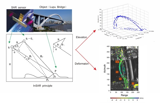
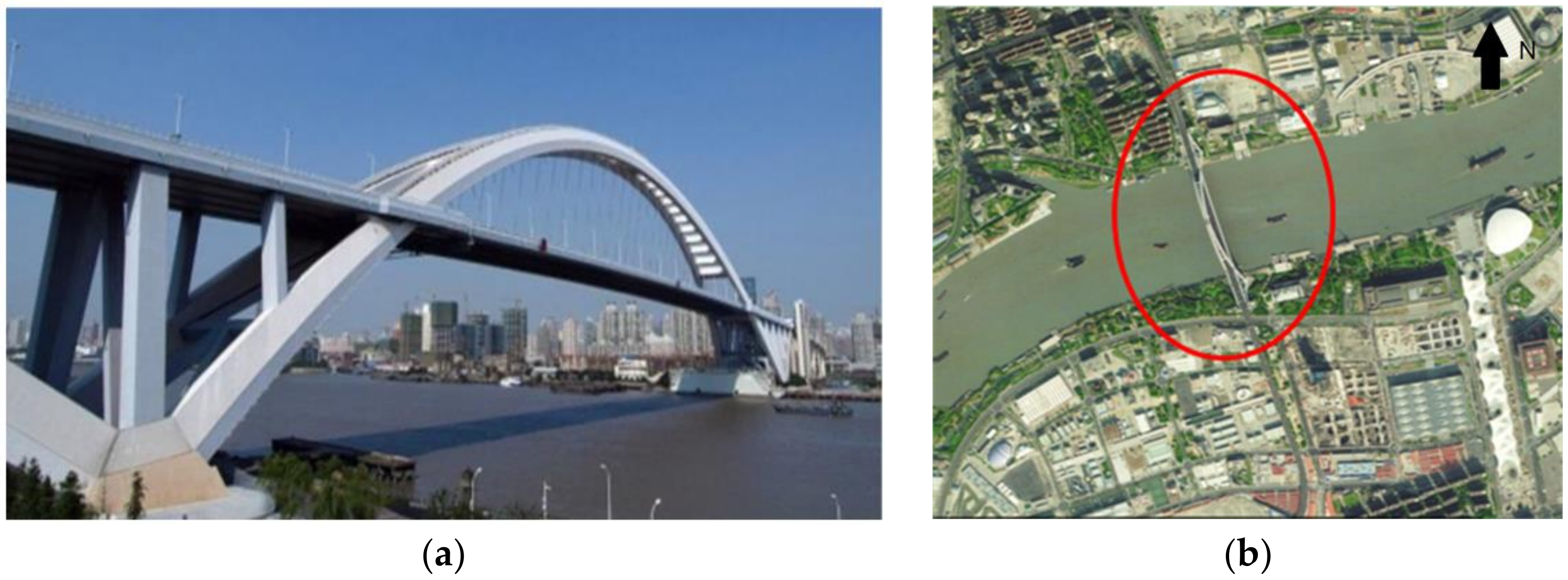
The research area is the Lupu Bridge (Figure 1) in Shanghai, China. This bridge has been in operation since 2003. The bridge is about 750 m long and 100 m tall. As the first arch bridge on the Huangpu River and the world’s second longest span all-steel arch bridge at that time, the Lupu Bridge soon became a famous scenic spot in Shanghai. The bridge’s axis is almost perpendicular to the radar line of sight (LOS) direction. Since the bridge structure is rather large, and the PS points of the bridge are sparse, it is quite difficult to form a connected PS network and resolve the arcs by the traditional PSI method.

Thirty-five (35) ascending X-band Cosmo-SkyMed SAR images are used. The key parameters of the images are shown in

Table 1. Parameters of the ascending Cosmo-SkyMed images.

Time Range	Number of Scenes	Azimuth Lines	Range Columns	Incident Angle (°)	Heading (°)	Azimuth Resolution (m)	Range Resolution (m)
10 December 2008–6 November 2010	35	400	250	40	−10.34	2.25	1.25

.

2.2. Data Processing Chain

2.2.1. Long–Short Baseline Iteration PSInSAR Method

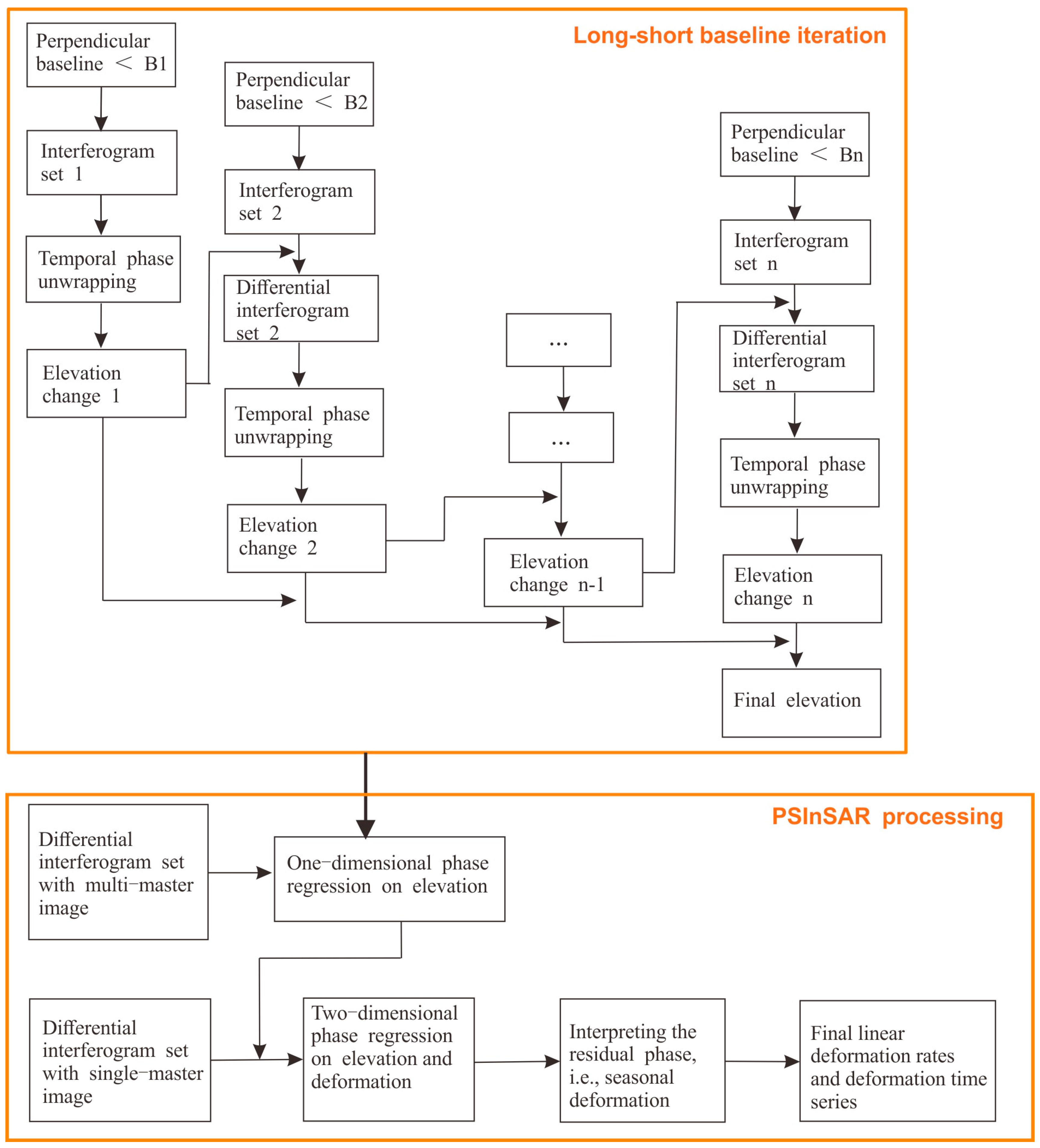
Figure 2 shows the workflow of the proposed method. As there is no accurate DSM data available, it is difficult to perform traditional two-dimensional phase unwrapping as the initial elevation value contributes considerably to the convergence of the algorithm. Therefore, the long–short baseline iteration PSInSAR method is applied for one-dimensional, accurate elevation extraction. Only interferometric pairs with a short temporal baseline are selected assuming no deformation exists. The thresholds of the interferometric perpendicular baseline in each iteration are loosened gradually as shown in

Table 2. Interferometric perpendicular baseline thresholds in a long–short baseline permanent scatterer interferometric synthetic aperture radar (PSInSAR) iteration.

Iteration Round	Temporal Baseline (Day)	Perpendicular Baseline (m)	Number of Interferometric Pairs	Number of Arcs Used in the Net	Elevation Ambiguity (m)
1	<65	<50	8	1320	150.0
2	<65	<200	38	1271	37.6
3	<65	<360	58	1395	20.9
4	<65	<600	77	1233	12.5
5	<65	<1000	119	1237	7.5

to improve the elevation accuracy. Note that the elevation ambiguity $∆\mathrm{h}$ is calculated from the perpendicular baseline,

$$∆\mathrm{h}=\frac{\mathsf{\lambda }\times \mathsf{\gamma }\times \sin \mathsf{\theta }}{2\mathrm{b}}$$

(1)

where $∆\mathrm{h}$ is the elevation ambiguity, i.e., the elevation change when the phase varies by 2π; $\mathsf{\lambda }$ is the radar wavelength; $\mathsf{\gamma }$ is the range between the satellite and the illuminating scene; $\mathsf{\theta }$ is the incident angle; and $\mathrm{b}$ is the perpendicular baseline.

The selection of PSs is conducted in GAMMA software using criteria such as the mean/standard deviation ratio, the minimum intensity, and coherence. In general, the PSs on the bridge are distributed along both the arches and the pavement of the bridge deck. Based on the PSs, an initial Delaunay triangular network is formed with 1700 arcs. As the large elevation differences between the arches and the deck are likely to result in the transmission and accumulation of elevation errors in the network adjustment, long arcs or those with poor coherence are screened out. Subsequently, phase unwrapping and network adjustment are carried out. In each iteration, the elevation of the PS on the deck with minimum azimuth is set as the reference. This value is 53.6 m, based on the bridge model offered by the official Lupu Bridge maintenance company. After five iterations, with a perpendicular baseline threshold condition of 1000 m, the PSs elevation corrections become very small; therefore, the elevation values obtained in the fifth iteration are considered the final solution.

2.2.2. The LLL Lattice Reduction Algorithm

InSAR phase unwrapping can be considered as a mixed integer least squares problem. The LLL lattice reduction algorithm separates the unknowns into an integer part and a real part, solving the integer part first and then the real part. In this way, the LLL algorithm provides a fast and numerically reliable routine to the mixed integer least squares problem.

y = Ax + Bz + δ

(2)

where x is a real unknown vector with k elements, $\mathrm{x}\in {\mathrm{R}}^{k*1}$; z is an integer unknown vector with n elements, $\mathrm{z}\in {\mathrm{Z}}^{n*1}$; $\mathrm{A}\in {\mathrm{R}}^{\mathrm{m}*\mathrm{k}}$ and $\mathrm{B}\in {\mathrm{R}}^{\mathrm{m}*\mathrm{n}}$ are known coefficient matrices with full column rank; m is the number of observations; and $\mathrm{y}\in {\mathrm{R}}^{\mathrm{m}*1}$ is the vector of observations. Z represents the set of integers; R represents the set of real numbers; δ is the noise vector. The aim is to solve for the unknowns x and z based on the known matrices A, B, and observations y. The solutions should minimize the 2-norm of vector $\mathrm{y}-\mathrm{Ax}-\mathrm{Bz}$:

$$\underset{\mathrm{x}\in {\mathrm{R}}^{\mathrm{k}},\mathrm{z}\in {\mathrm{Z}}^{\mathrm{n}}}{\min }\Vert \mathrm{y}-\mathrm{Ax}-{\mathrm{Bz}\Vert }_2^2$$

(3)

If matrix A has QR factorization (A decomposition of a matrix A into a product A = QR of an orthogonal matrix Q and an upper triangular matrix R),

$$\mathrm{A}=\left[\begin{array}{cc}{\mathrm{Q}}_{\mathrm{A}}& {\overline{\mathrm{Q}}}_{\mathrm{A}}\end{array}\right]\left[\begin{array}{c}{\mathrm{R}}_{\mathrm{A}}\\ 0\end{array}\right]$$

(4)

where $\left[\begin{array}{cc}{\mathrm{Q}}_{\mathrm{A}}& {\overline{\mathrm{Q}}}_{\mathrm{A}}\end{array}\right]\in {\mathrm{R}}^{\mathrm{m}*\mathrm{m}}$ is orthogonal, and ${\mathrm{R}}_{\mathrm{A}}\in {\mathrm{R}}^{\mathrm{k}*\mathrm{k}}$ is a nonsingular upper triangular matrix. Then

$$\begin{gathered} \Vert \mathrm{y}-\mathrm{Ax}-{\mathrm{Bz}\Vert }_2^2=\Vert {\left[\begin{array}{c}{\mathrm{Q}}_{\mathrm{A}}^{\mathrm{T}}\\ {\overline{\mathrm{Q}}}_{\mathrm{A}}^{\mathrm{T}}\end{array}\right]\mathrm{y}-\left[\begin{array}{c}{\mathrm{R}}_{\mathrm{A}}\\ 0\end{array}\right]\mathrm{x}-\left[\begin{array}{c}{\mathrm{Q}}_{\mathrm{A}}^{\mathrm{T}}\mathrm{B}\\ {\overline{\mathrm{Q}}}_{\mathrm{A}}^{\mathrm{T}}\mathrm{B}\end{array}\right]\mathrm{z}\Vert }_2^2 \\ =\Vert {\mathrm{Q}}_{\mathrm{A}}^{\mathrm{T}}\mathrm{y}-{\mathrm{R}}_{\mathrm{A}}\mathrm{x}-{\mathrm{Q}}_{\mathrm{A}}^{\mathrm{T}}{\mathrm{Bz}\Vert }_2^2+\Vert {\overline{\mathrm{Q}}}_{\mathrm{A}}^{\mathrm{T}}\mathrm{y}-{\overline{\mathrm{Q}}}_{\mathrm{A}}^{\mathrm{T}}{\mathrm{Bz}\Vert }_2^2 \end{gathered}$$

(5)

If z is fixed, there must be an appropriate $\mathrm{x}\in {\mathrm{R}}^{\mathrm{k}*1}$ that ensures that the first term ($\Vert {\mathrm{Q}}_{\mathrm{A}}^{\mathrm{T}}\mathrm{y}-{\mathrm{R}}_{\mathrm{A}}\mathrm{x}-{\mathrm{Q}}_{\mathrm{A}}^{\mathrm{T}}{\mathrm{Bz}\Vert }_2^2\ge 0$) in Equation (5) is 0 so as to satisfy the minimization requirement of Equation (3). Therefore, the problem can be decomposed into the following two problems,

1. An ordinary integer least squares problem to calculate $\widehat{\mathrm{z}}$

$$\underset{\mathrm{z}\in {\mathrm{Z}}^{\mathrm{n}}}{\min }\Vert {\overline{\mathrm{Q}}}_{\mathrm{A}}^{\mathrm{T}}\mathrm{y}-{\overline{\mathrm{Q}}}_{\mathrm{A}}^{\mathrm{T}}{\mathrm{Bz}\Vert }_2^2$$

(6)

Specifically, a reduction algorithm and a search algorithm are presented to obtain the integer z which satisfies Equation (6).

2. With z known, Equation (3) becomes a least squares problem. With $\hat{\mathrm{z}}$ brought back into Equation (5) and setting the first term into 0, $\hat{\mathrm{x}}$ can be obtained from

$${\mathrm{R}}_{\mathrm{A}}\mathrm{x}={\mathrm{Q}}_{\mathrm{A}}^{\mathrm{T}}\mathrm{y}-{\mathrm{Q}}_{\mathrm{A}}^{\mathrm{T}}\mathrm{B}\hat{\mathrm{z}}$$

(7)

For simplicity, the above problem 1 is noted as:

$$\underset{\mathrm{z}\in {\mathrm{Z}}^{\mathrm{n}}}{ \min }\Vert \mathrm{y}-{\mathrm{Bz}\Vert }_2^2$$

(8)

where y is a known vector; z is the least squares solution required; and $\mathrm{Bz}$ is a vector in the grid. Thus, seeking a solution for Equation (8) can be interpreted as searching for the grid vector that is nearest to y. This is a closest vector problem (CVP), which has been proven to be an NP-hard (non-deterministic polynomial hard) problem. To make the search process simple and efficient, many reduction methods have been proposed. In this study, we use the LLL method, which has two steps,

• Reduction

First, using a minimum main-element method, the QR decomposition of matrix B is carried out to transform it into an upper triangular matrix R and an orthogonal matrix Q. Second, the non-diagonal elements in R are reduced using an integer Gaussian transform to remove any correlation and enable efficient searching. Third, the columns are rearranged using the minimum-column pivoting strategy to meet the LLL reduction criterion.

• Search

After reduction, we need to search for the optimal integer solution $\mathrm{z}\in {\mathrm{Z}}^{\mathrm{n}}$ to satisfy $\underset{\overline{\mathrm{z}}\in {\mathrm{Z}}^{\mathrm{n}}}{\min }\Vert \overline{\mathrm{y}}-{\mathrm{R}\overline{\mathrm{z}}\Vert }_2^2$. Given a threshold β, we assume that the optimal integer solution z satisfies

$$\mathrm{f}\left(\mathrm{z}\right)\triangleq \Vert \mathrm{y}-{\mathrm{Rz}\Vert }_2^2<\mathsf{\beta }$$

(9)

This corresponds to searching for the optimal solution within an ellipsoid.

R is then decomposed into the first (n − 1)-order submatrix and the last line, and y is decomposed into the (n − 1)-dimensional sub-vector and the last element. Thus,

$$\begin{gathered} \Vert \mathrm{y}-{\mathrm{Rz}\Vert }_2^2=\Vert \left(\begin{array}{c}{\mathrm{y}}_1\\ {\mathrm{y}}_{\mathrm{n}}\end{array}\right)-\left(\begin{array}{cc}{\mathrm{R}}_1& {\mathrm{r}}_{1:\mathrm{n}-1,\mathrm{n}}\\ 0& {\mathrm{r}}_{\mathrm{nn}}\end{array}\right){\left(\begin{array}{c}{\mathrm{z}}_1\\ {\mathrm{z}}_{\mathrm{n}}\end{array}\right)\Vert }_2^2 \\ =\Vert \left({\mathrm{y}}_1-{\mathrm{z}}_{\mathrm{n}}{\mathrm{r}}_{1:\mathrm{n}-1,\mathrm{n}}\right)-{\mathrm{R}}_1{\mathrm{z}}_1{\Vert }_2^2+{\left({\mathrm{y}}_{\mathrm{n}}-{\mathrm{r}}_{\mathrm{nn}}{\mathrm{z}}_{\mathrm{n}}\right)}^2 \end{gathered}$$

(10)

To satisfy Equation (9), the following conditions need to be met,

$${\left({\mathrm{y}}_{\mathrm{n}}-{\mathrm{r}}_{\mathrm{nn}}{\mathrm{z}}_{\mathrm{n}}\right)}^2<\mathsf{\beta }$$

(11)

and

$$\Vert \left({\mathrm{y}}_1-{\mathrm{z}}_{\mathrm{n}}{\mathrm{r}}_{1:\mathrm{n}-1,\mathrm{n}}\right)-{\mathrm{R}}_1{\mathrm{z}}_1{\Vert }_2^2<\mathsf{\beta }-{\left({\mathrm{y}}_{\mathrm{n}}-{\mathrm{r}}_{\mathrm{nn}}{\mathrm{z}}_{\mathrm{n}}\right)}^2$$

(12)

Equation (12) is an (n − 1)-dimensional integer least squares problem, and the corresponding search radius is $\mathsf{\rho }=\sqrt{(\mathsf{\beta }-{\left({\mathrm{y}}_{\mathrm{n}}-{\mathrm{r}}_{\mathrm{nn}}{\mathrm{z}}_{\mathrm{n}}\right)}^2)}$. The integer solution to Equation (11) falls within $\left[({\mathrm{y}}_{\mathrm{n}}-\mathsf{\beta })/{\mathrm{r}}_{\mathrm{nn}},({\mathrm{y}}_{\mathrm{n}}+\mathsf{\beta })/{\mathrm{r}}_{\mathrm{nn}}\right]$. Using this algorithm recursively, we can solve the upper triangular integer least squares problem.

Once the p optimal integer solutions $\hat{\mathrm{z}}$ are obtained, we can use the following upper triangular matrix to solve for the corresponding p real solutions: ${\mathrm{R}}_{\mathrm{A}}\hat{\mathrm{x}}={\mathrm{Q}}_{\mathrm{A}}^{\mathrm{T}}\left({\mathrm{ye}}^{\mathrm{T}}-\mathrm{B}\hat{\mathrm{z}}\right)$, where $\mathrm{e}={\left[1,\cdots ,1\right]}^{\mathrm{T}}ϵ{\mathrm{R}}^{\mathrm{p}}$.

2.2.3. LLL Lattice Reduction Algorithm Used for PSInSAR

When applying the above LLL lattice reduction algorithm to PSInSAR data processing, by contrast, the phase ambiguities correspond to the integer unknowns, while the elevation error and the linear deformation rates correspond to the real unknowns, and the interferometric phases correspond to the observations in Section 2.2.2.

Assume that there are m + 1 SAR images of the same area, obtained at time t₁, …, t_m+1, respectively. One of the images is chosen as the master image and the other m images are the slave images, to form m interferograms. The unwrapped phase between pixel i and pixel j in interferogram p is expressed as

$$∆{\varnothing }_{\mathrm{ij}}^{\mathrm{p}}={\mathsf{\alpha }}^{\mathrm{p}}\times {\mathrm{v}}_{\mathrm{ij}}+{\mathsf{\beta }}^{\mathrm{p}}\times {\mathrm{h}}_{\mathrm{ij}}+2\mathsf{\pi }\times \mathrm{z}+\mathsf{\delta }$$

(13)

where ${\mathrm{v}}_{\mathrm{ij}}$ and ${\mathrm{h}}_{\mathrm{ij}}$ are the relative displacement rate and relative elevation error between the two pixels, respectively. ${\mathsf{\beta }}^{\mathrm{p}}$ changes with the perpendicular baseline, and ${\mathsf{\alpha }}^{\mathrm{p}}$ changes with the temporal baseline. z is the unknown number of whole phase cycles, and $\mathsf{\delta }$ is the noise resulting possibly from decorrelation error, nonlinear deformation, thermal noise, and so on. Note that the atmospheric phase is considered to be correlated in space and can be significantly reduced by differencing interferometric phases between adjacent PSs to form an arc observation.

As an arc in an interferogram contains one-integer ambiguity, together with real unknowns ${\mathrm{v}}_{\mathrm{ij}}$ and ${\mathrm{h}}_{\mathrm{ij}}$, there are m + 2 unknowns in the m interferograms corresponding to the arc. As there are only m observations, the observation equations formed according to Equation (13) have rank defects. To solve this problem, the initial values of two unknown parameters are assumed to be equal to 0, i.e.,

$$\{\begin{array}{c}{\mathrm{h}}_{\mathrm{ij}}=0\\ {\mathrm{v}}_{\mathrm{ij}}=0\end{array}$$

(14)

and will be updated iteratively. The new observation equations can be expressed as follows:

$$\mathrm{y}=\left(\begin{array}{c}\mathrm{A}1\\ \mathrm{A}2\end{array}\right)\mathrm{x}+\left(\begin{array}{c}\mathrm{B}1\\ \mathrm{B}2\end{array}\right)\mathrm{z}+\mathsf{\delta }$$

(15)

where A1 has m rows, and its two columns are ${\left[{\mathsf{\alpha }}^1,\dots ,{\mathsf{\alpha }}^{\mathrm{m}}\right]}^{\mathrm{T}}$ and ${\left[{\mathsf{\beta }}^1,\dots ,{\mathsf{\beta }}^{\mathrm{m}}\right]}^{\mathrm{T}}$, respectively. A2 is a 2 × 2 identity matrix. The real unknowns x include ${\mathrm{v}}_{\mathrm{ij}}$ and ${\mathrm{h}}_{\mathrm{ij}}$. B1 is an m × m identity matrix times 2π. B2 is a 2 × m zero matrix. If the signal-to-noise ratio of the observations is high, the solution can be found with a few iterations.

3. Results and Discussion

3.1. Bridge Elevation Extraction

At first, only interferometric pairs with a short temporal baseline are selected assuming no deformation exists, and only the relative elevation errors are considered as the real unknowns in the one-dimensional elevation extraction step with LLL. The thresholds of the interferometric perpendicular baseline length in each iteration are loosened gradually, as shown in Table 2, to improve the elevation estimation accuracy obtained.

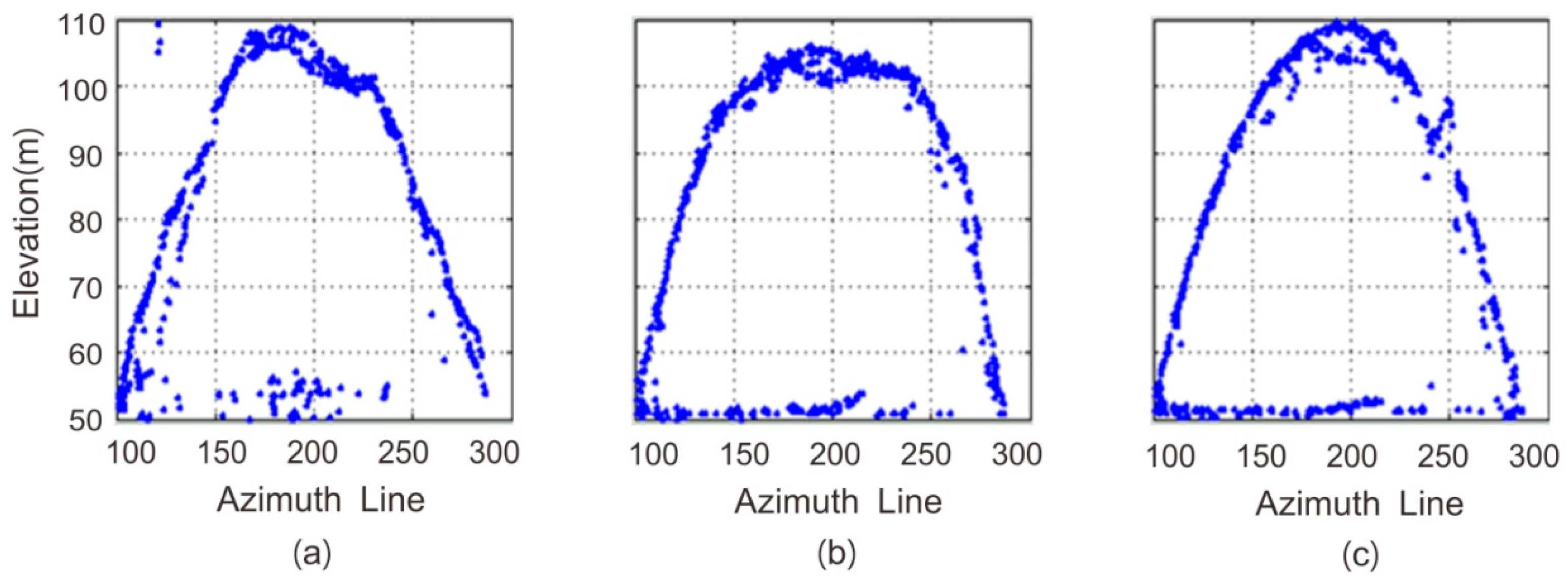
Figure 3 shows the side views of the PS elevations on the bridge obtained in iterations 1 (B_⊥ < 50 m), 3 (B_⊥ < 360 m), and 5 (B_⊥ < 1000 m), respectively. In iteration 1, it is obvious that the elevation variations are relatively larger and the elevations on the arch are discontinuous, even with some obvious errors. However, with the loosening of the spatial baseline threshold and the increase of iterations, the elevations become smoother. The elevations obtained in iteration 5 are accepted as the final solution.

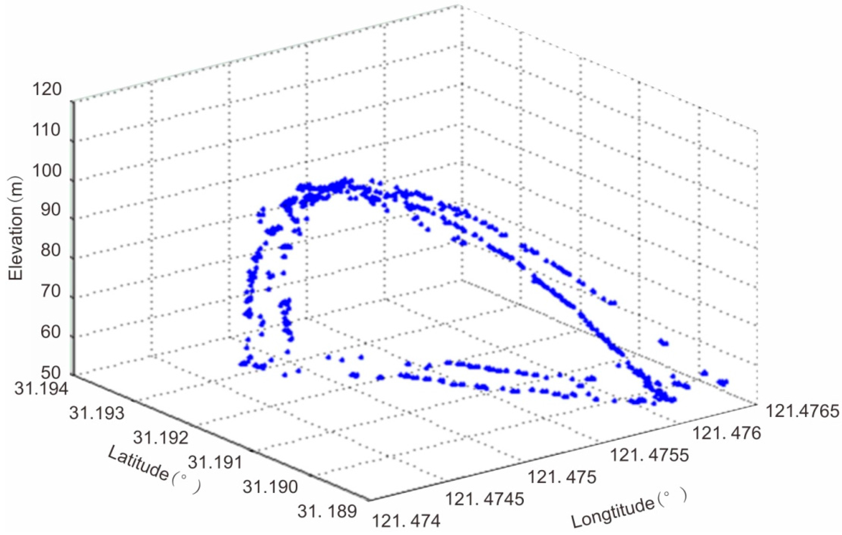
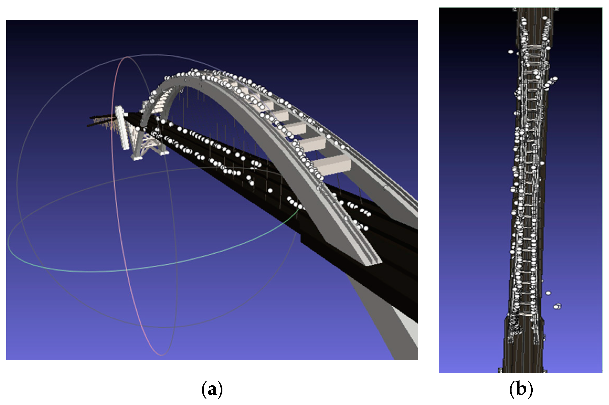
Figure 4 shows the elevations of PSs on the bridge obtained in iteration 5 after geocoding (three-dimensional (3D) view). The results clearly show the bridge arches and the deck. In order to further evaluate the accuracy of the obtained elevations, two external bridge datasets are used for comparison. One is the official bridge model obtained from the Shanghai Lupu Bridge Investment Development Co., Ltd. (No. 449, Yaohua Road, Shanghai, China). Three key parameters of the bridge structure (namely, maximum arch elevation, minimum deck elevation, and maximum deck elevation) obtained in iterations 1, 3, and 5 are compared with the official bridge model dataset (

Table 3. Key parameters of the estimated bridge structure from iterations 1, 3, and 5 compared with the bridge model data (only direct measurements are listed).

	Iteration 1	Iteration 3	Iteration 5	Official Model
Maximum arch elevation (m)	109.1	106.0	109.6	109.35
Minimum deck elevation (m)	41.1	47.3	50.1
Maximum deck elevation (m)	59.1	54.2	53.2
Mean deck elevation (m)				53.60

). The accuracy of the estimated elevations improves with the number of iterations; the final estimated elevations from iteration 5 are in good agreement with the bridge model. Note that Table 3 only presents a rough comparison, as it is difficult to match the PSs with their exact location in the bridge model, and therefore the elevation differences between the InSAR solution and the model do not necessarily represent the accuracy of the proposed method. The second external bridge dataset is downloaded from Google 3D Warehouse. The 3D PSs are transformed to the model coordinates for visualization in the Meshlab software. As shown in Figure 5, the arch shape and the location of the PSs are in excellent agreement.

3.2. Bridge Deformation Extraction

As shown in [29], the Lupu Bridge is an all-welded steel arch bridge connected by a set of components with a misalignment error of less than 1 mm. Moreover, even with nearly 20 arch ribs and a span of more than 500 m connecting Puxi and Pudong, the axial deviation of the central arch joints is less than 5 mm.

In fact, it is challenging to interpret InSAR-derived deformation results of man-made structures, particularly bridges, because it can be difficult to separate the major components of the InSAR phase, such as the linear deformation rates, seasonal deformation, elevation of structures, and atmosphere phase screen (APS). For example, the elevation-related atmospheric phase and the temperature-related deformation tend to have the same pattern. The elevation errors leak easily to deformation solutions. A few InSAR time series studies have investigated the thermal expansion of bridges and other structures [30,31,32,33,34,35]; however, many technical details are yet to be resolved.

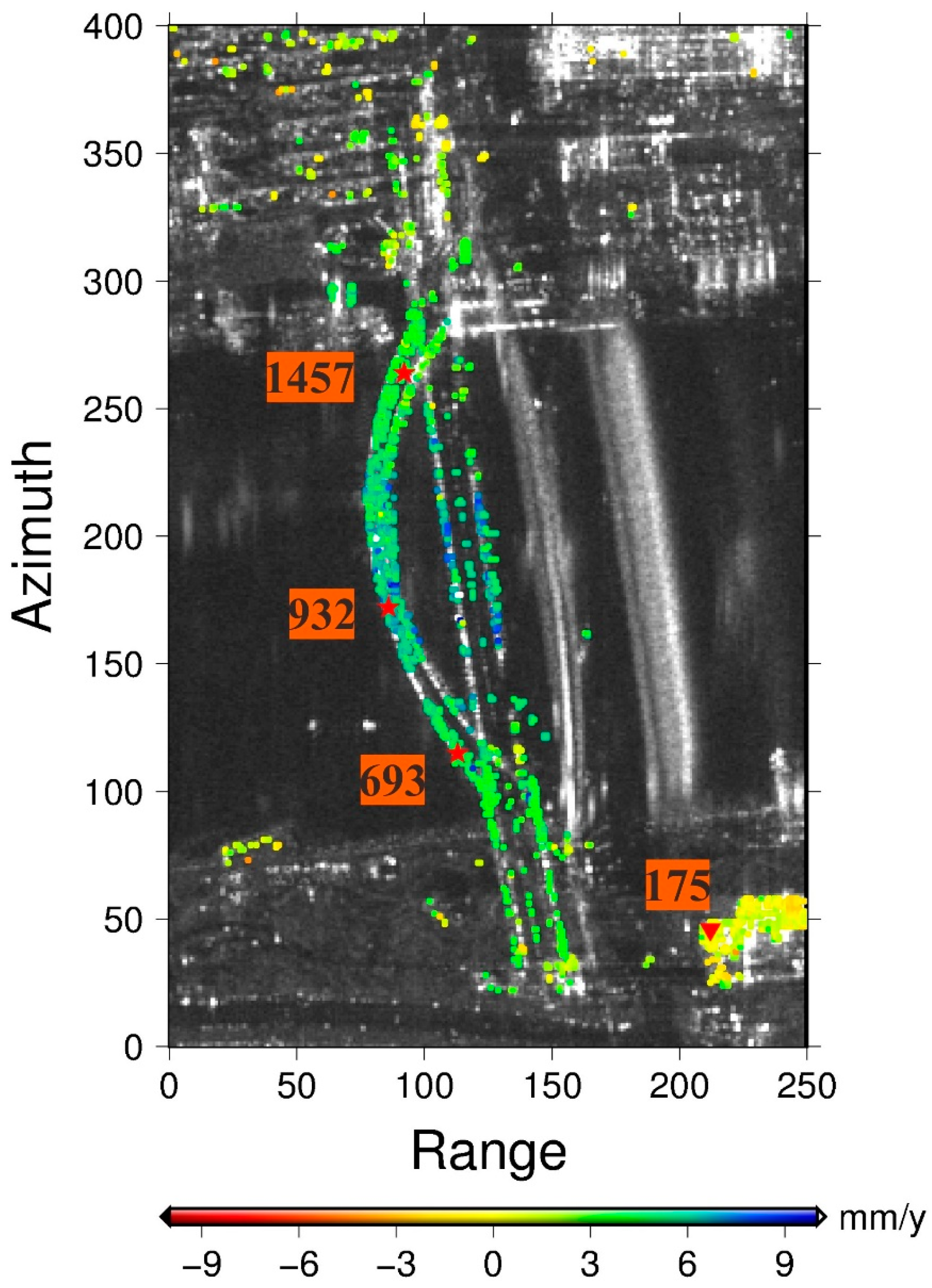
In the Lupu Bridge case, once the elevations of the PSs are resolved with suitable accuracy, they are then used in a two-dimensional phase regression involving both elevation and linear deformation, and to obtain the linear deformation map as in Figure 6. By the way, PS No. 175 on the riverside is chosen as the reference point. As the research area is relatively small, the APS is neglected.

As shown in Figure 6, the linear deformation rates of the main part of the bridge are uniform, indicating that the bridge is stable as a whole. The LOS deformation rates compared to the reference point No. 175 vary from 4 to 7 mm per year during the SAR image acquisition period. Note that a positive value represents motion away from the satellite along the LOS, while a negative value indicates motion towards the satellite along the LOS. Progressive deformation appears on the two bridge arches and bridge deck. The largest deformation rates occur at the central part of the arches (7 mm per year) and the bridge deck (9 mm per year).

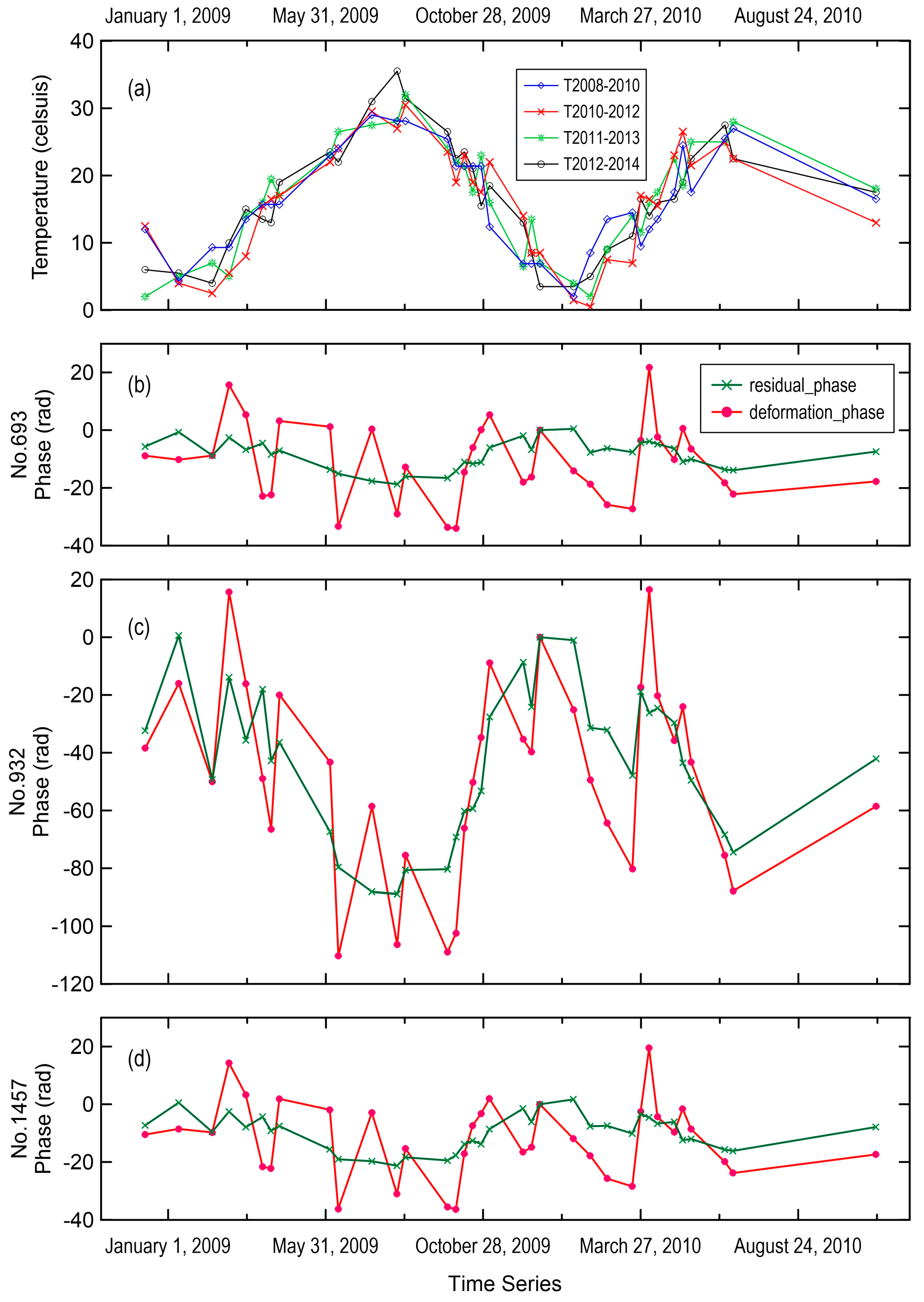
The thermal expansion of metallic or reinforced concrete structures can significantly affect the interferometric phase signature [36]. Typically, thermal dilation provides progressive patterns due to its accumulation over the structure’s length. This is in agreement with our result. To further study thermal expansion effects on the deformation results, we collected temperature records of Shanghai during the SAR image acquisition period. Unfortunately, only some scattered monthly averaged temperature records can be found on the internet for the period, i.e., from December 2008 to November 2010. The SAR sensor passed over Shanghai at about 06:00 Beijing time. However, if we calculate the average temperature on the date of the data acquisition two, three, and four years later (T2010–2012, T2011–2013, T2012–2014 in Figure 7a) and extrapolate the monthly temperature during 2008 to 2010 (T2008–2010 in Figure 7a), the trends of variation of the temperature are almost the same. Thus, the interpolated temperature (T2008–2010) is used for the seasonal deformation analysis.

Three PSs (No. 693, 932, and 1457), whose locations are shown in Figure 6, are chosen for a more detailed seasonal deformation analysis. In the two-dimensional phase regression as shown in the last line of the bottom box in Figure 2, the unwrapped deformation phase time series (red dots) and the residual time series (green crosses) of these three points are shown in Figure 7b–d. Note that the unwrapped deformation phase time series are calculated by removing the elevation phase from the unwrapped interferometric phase, while the residual unwrapped phase is obtained by removing both the linear deformation and elevation phase from the unwrapped phase.

Both the unwrapped deformation phase time series and residual time series of the three points are used to calculate the correlation coefficients with the interpolated temperature (T2008–2010) and the results are listed in

Table 4. Coefficients between the residual unwrapped phase/unwrapped deformation phase and temperature variations.

PS Point Number	Location	Correlation Coefficient (Residual Unwrapped Phase vs. Temperature)	Correlation Coefficient (Unwrapped Deformation Phase vs. Temperature)
693	Southern end of arch	−0.9225	−0.2526
932	Center	−0.9163	−0.6460
1457	Northern end of arch	−0.9240	−0.3421

. In Table 4, the residual unwrapped phase time series corresponding to the three PSs have a strong negative correlation with the temperature. The correlation coefficients of all the three target points are larger than 0.9. When the phases of the linear deformation and the minor elevation correction are added back, the unwrapped phase time series have a much weaker negative correlation with the temperature, with the correlation coefficients ranging from 0.2526 to 0.646, with 0.646 corresponding to the PS at the center of the bridge arches, indicating that this PS was affected much more by the temperature than the other two PSs.

As expected, the central parts of the bridge arches and the bridge deck were experiencing the largest deformation.

4. Conclusions and Outlook

We use a long–short baseline iteration method for elevation extraction in PSInSAR data processing to overcome the high-phase-gradient problem in a case where no DSM is available, so as to improve the accuracy of the estimated deformation rates. The LLL lattice reduction algorithm is used to rapidly reduce the search radius, compress the search space, and improve the success rate of resolving the ambiguities in phase unwrapping. To validate the method, elevations of 577 PSs on the Lupu Bridge have been obtained and compared with elevation data of the bridge model. The results are in excellent agreement. Besides, the linear deformation rates and seasonal deformation of the PSs have been extracted from InSAR deformation time series, which indicates that the bridge is stable in general, although symmetric progressive deformation has been found on the bridge arches and the bridge deck. The results agree with the Lupu Bridge design, where the arch joints would absorb most of the thermal deformation to mitigate the thermal dilation of the bridge as much as possible. Compared to the traditional PSInSAR approach, our method obtained more accurate elevation estimations. Consequently, the deformation estimation results are also more reliable.

As a whole, multitemporal InSAR is a useful tool for elevation reconstruction and the health monitoring of large infrastructures, such as bridges, dams, and high-rise buildings. Future work should be focused on interpreting the deformation; for example, linking individual PSs with the local structural elements and evaluating the results. It should also be interesting to consider to model the temperature-related deformation in the InSAR observation equation and to carry out close comparison of the results with in-situ measurements.

References

- Ferretti, A.; Prati, C.; Rocca, F. Permanent scatterers in SAR interferometry. IEEE Trans. Geosci. Remote Sens. 2001, 39, 8–20. [Google Scholar] [CrossRef]
- Kampes, B.M. Radar Interferometry: Persistent Scatterer Technique; Springer: Dordrecht, The Netherlands, 2006. [Google Scholar]
- Gernhardt, S.; Bamler, R. Deformation monitoring of single buildings using meter-resolution SAR data in PSI. ISPRS J. Photogramm. Remote Sens. 2012, 73, 68–79. [Google Scholar] [CrossRef]
- Zhu, X.X. Very High Resolution Tomographic SAR Inversion for Urban Infrastructure Monitoring—A Sparse and Nonlinear Tour. Ph.D. Thesis, University of München, München, Germany, 2011. [Google Scholar]
- Adam, N.; Gonzalez, F.R.; Parizzi, A.; Brcic, R. Wide area persistent scatterer interferometry: Current developments, algorithms and examples. In Proceedings of the 2013 IEEE International Geoscience and Remote Sensing Symposium (IGRASS), Melbourne, Australia, 21–26 July 2013; pp. 1857–1860. [Google Scholar]
- Gernhardt, S. High Precision 3D Localization and Motion Analysis of Persistent Scatterers Using Meter-Resolution Radar Satellite Data. Ph.D. Thesis, University of München, München, Germany, 2012. [Google Scholar]
- Zhu, X.X.; Shahzad, M. Facade reconstruction using multiview spaceborne TomoSAR point clouds. IEEE Trans. Geosci. Remote Sens. 2014, 52, 3541–3552. [Google Scholar] [CrossRef]
- Bakon, M.; Perissin, D.; Lazecky, M.; Papco, J. Infrastructure nonlinear deformation monitoring via satellite radar interferometry. In Proceedings of the Conference on Enterprise Information Systems (ICEIS), Lisbon, Portugal, 27–30 April 2014; pp. 294–300. [Google Scholar]
- Lazecky, M.; Perissin, D.; Bakon, M.; Sousa, J.J.M.; Hlavacova, I.; Real, N. Potential of satellite InSAR techniques for monitoring of bridge deformations. Presented at the Joint Urban Remote Sensing Event, Lausanne, Switzerland, 1 April 2015. [Google Scholar]
- Goldstein, R.M.; Zebker, H.A.; Werner, C.L. Satellite radar interferometry: Two-dimensional phase unwrapping. Radio Sci. 1988, 23, 713–720. [Google Scholar] [CrossRef]
- Flynn, T.J. Consistent 2-D phase unwrapping guided by a quality map. In Proceedings of the 1996 IEEE International Geoscience and Remote Sensing Symposium (IGRASS), Piscataway, NE, USA, 31 May 1996; pp. 2057–2059. [Google Scholar]
- Xu, W.; Cumming, I. A region-growing algorithm for InSAR phase unwrapping. IEEE Trans. Geosci. Remote Sens. 1999, 37, 124–134. [Google Scholar] [CrossRef]
- Carballo, G.F.; Fieguth, P.W. Probabilistic cost functions for network flow phase unwrapping. IEEE Trans. Geosci. Remote Sens. 2000, 38, 2192–2201. [Google Scholar] [CrossRef]
- Chen, C.W. Statistical-Cost Network-Flow Approaches to Two-Dimensional Phase Unwrapping for Radar Interferometry. Ph.D. Thesis, Stanford University, Stanford, CA, USA, 2001. [Google Scholar]
- Hooper, A.; Zebker, H.A. Phase unwrapping in three dimensions with application to InSAR time series. J. Opt. Soc. Am. A 2007, 24, 2737–2747. [Google Scholar] [CrossRef]
- Herráez, M.A.; Burton, D.R.; Lalor, M.J.; Gdeisat, M.A. Fast two-dimensional phase-unwrapping algorithm based on sorting by reliability following a noncontinuous path. Appl. Opt. 2002, 41, 7437–7444. [Google Scholar] [CrossRef] [PubMed]
- Bioucas-Dias, J.M.; Valadao, G. Phase unwrapping via graph cuts. IEEE Trans. Image Process. 2007, 16, 698–709. [Google Scholar] [CrossRef] [PubMed]
- Li, C.; Zhu, D.Y. A residue-pairing algorithm for InSAR phase unwrapping. Prog. Electromagn. Res. 2009, 95, 341–354. [Google Scholar] [CrossRef]
- Lenstra, A.K.; Lenstra, H.W.; Lovász, L. Factoring polynomials with rational coefficients. Math. Ann. 1982, 261, 515–534. [Google Scholar] [CrossRef]
- Fincke, U.; Pohst, M. On reduction algorithms in non-linear integer mathematical programming. In Proceedings of the Operation Research, Mannheim, Germany, 21–23 September 1983; pp. 289–295. [Google Scholar]
- Lagarias, J.C. Knapsack Public Key Cryptosystems and Diophantine Approximation; Springer US: New York, NY, USA, 1984. [Google Scholar]
- Coppersmith, D. Small solutions to polynomial equations and low exponent vulnerabilities. J. Cryptol. 1997, 10, 223–260. [Google Scholar] [CrossRef]
- Kaltofen, E.; Yui, N. Explicit Construction of the Hilbert Class Fields of Imaginary Quadratic Fields by Integer Lattice Reduction; Springer US: New York, NY, USA, 1991. [Google Scholar]
- Liu, J.N.; Yu, X.W.; Zhang, X.H. GNSS ambiguity resolution using the lattice theory. Acta Geod. Cartogr. Sin. 2012, 41, 636–645. [Google Scholar]
- Zhou, L.F. Monitoring Ground Deformation in Urban Major Project Area with High-Resolution Persistent Scatterer SAR Interferometry. Ph.D. Thesis, Zhejiang University, Hangzhou, China, 2014. [Google Scholar]
- Robertson, A.E. Multi-Baseline Interferometric SAR for Iterative Height Estimation. Master’s Thesis, Brigham Young University, Provo, UT, USA, 1998. [Google Scholar]
- Thompson, D.G.; Robertson, A.E.; Arnold, D.V.; Long, D.G. Multi-baseline interferometric SAR for iterative height estimation. In Proceedings of the 1999 IEEE International Geoscience and Remote Sensing Symposium (IGRASS), Hamburg, Germany, 28 June–2 July 1999; pp. 251–253. [Google Scholar]
- Pieraccini, M.; Luzi, G.; Atzeni, C. Terrain mapping by ground-based interferometric radar. IEEE Geosci. Remote Sens. Lett. 2001, 39, 2176–2181. [Google Scholar] [CrossRef]
- Academician Lin Yuanpei Tells the History of Shanghai Bridges. Available online: http://tieba.baidu.com/p/1108985575 (accessed on 14 June 2011).
- Reale, D.; Fornaro, G.; Pauciullo, A. Extension of 4-D SAR imaging to the monitoring of thermally dilating scatterers. IEEE Trans. Geosci. Remote Sens. 2013, 51, 5296–5306. [Google Scholar] [CrossRef]
- Fornaro, G.; Reale, D.; Verde, S. Bridge thermal dilation monitoring with millimeter sensitivity via multidimensional SAR imaging. IEEE Geosci. Remote Sens. Lett. 2013, 10, 677–681. [Google Scholar] [CrossRef]
- Monserrat, O.; Crosetto, M.; Cuevas, M.; Crippa, B. The thermal expansion component of persistent scatterer interferometry observations. IEEE Geosci. Remote Sens. Lett. 2011, 8, 864–868. [Google Scholar] [CrossRef]
- Goel, K.; Gonzalez, F.R.; Adam, N.; Duro, J.; Gaset, M. Thermal dilation monitoring of complex urban infrastructure using high resolution SAR data. In Proceedings of the 2014 IEEE International Geoscience and Remote Sensing Symposium (IGRASS), Quebec, QC, Canada, 13–18 July 2014; pp. 954–957. [Google Scholar]
- Cuevas, M.; Monserrat, O.; Crosetto, M.; Crippa, B. A new product from persistent scatterer interferometry: The thermal dilation maps. In Proceedings of the 2011 Joint Urban Remote Sensing Event (JURSE), Munich, Germany, 11–13 April 2011; pp. 285–288. [Google Scholar]
- Montazeri, S.; Zhu, X.X.; Eineder, M.; Bamler, R. Three-Dimensional Deformation Monitoring of Urban Infrastructure by Tomographic SAR Using Multitrack TerraSAR-X Data Stacks. IEEE Trans. Geosci. Remote Sens. 2016, 54, 6868–6878. [Google Scholar] [CrossRef]
- Lazecky, M.; Hlavacova, I.; Bakon, M.; Sousa, J.J.; Perissin, D.; Patricio, G. Bridge Displacements Monitoring Using Space-Borne X-Band SAR Interferometry. IEEE J. Sel. Top. Appl. Earth Obs. Remote Sens. 2017, 10, 205–210. [Google Scholar] [CrossRef]
Figure 1.
Lupu Bridge: (a) side view; (b) top view (red circle surrounding the bridge) (Cr. Baidu).
Figure 2.
Workflow of the proposed InSAR processing method.
Figure 3.
Estimated permanent scatterer (PS) elevations on the bridge obtained in iterations 1 (B⊥ < 50 m) (a); 3 (B⊥ < 360 m) (b); and 5 (B⊥ < 1000 m) (c), respectively (Azimuth-Elevation plane).
Figure 4.
Elevations of PSs on the bridge from iteration 5 (three-dimensional (3D) view).
Figure 5.
PSs (white dots) superimposed on the bridge model in Meshlab: (a) side view; (b) top view.
Figure 6.
Linear deformation rates (in the line of sight (LOS) direction) of PSs. The labeled numbers are the IDs of chosen PSs. Red stars and the inverted triangle indicate the monitoring PSs (No. 693, 932, and 1457) and the reference PS (No. 175), respectively.
Figure 7.
(a) Temporal variations of temperature (T2008–2010: interpolated averaged daily temperature records on SAR data acquisition dates. T2010–2012, T2011–2013, T2012–2014: averaged daily temperature records on acquisition dates two, three, and four years later); (b–d): Unwrapped deformation phase time series (red dots) and residual time series (green crosses) of PS points 693, 932, and 1457 whose locations are shown in Figure 6.