
Rational PCR Reactor Design in Microfluidics

1
School of Engineering and Sciences, Tecnologico de Monterrey, Monterrey 64849, NL, Mexico
2
Autonomous Medical Devices Incorporated (AMDI), Santa Ana, CA 92704, USA
*
Author to whom correspondence should be addressed.
Micromachines 2023, 14(8), 1533; https://doi.org/10.3390/mi14081533
Submission received: 28 May 2023
/
Revised: 7 July 2023
/
Accepted: 13 July 2023
/
Published: 31 July 2023
(This article belongs to the Special Issue Recent Advances of Microfluidics for Biomedical Applications)
Abstract
:Limit of detection (LOD), speed, and cost for some of the most important diagnostic tools, i.e., lateral flow assays (LFA), enzyme-linked immunosorbent assays (ELISA), and polymerase chain reaction (PCR), all benefited from both the financial and regulatory support brought about by the pandemic. From those three, PCR has gained the most in overall performance. However, implementing PCR in point of care (POC) settings remains challenging because of its stringent requirements for a low LOD, multiplexing, accuracy, selectivity, robustness, and cost. Moreover, from a clinical point of view, it has become very desirable to attain an overall sample-to-answer time (t) of 10 min or less. Based on those POC requirements, we introduce three parameters to guide the design towards the next generation of PCR reactors: the overall sample-to-answer time (t); lambda (λ), a measure that sets the minimum number of copies required per reactor volume; and gamma (γ), the system’s thermal efficiency. These three parameters control the necessary sample volume, the number of reactors that are feasible (for multiplexing), the type of fluidics, the PCR reactor shape, the thermal conductivity, the diffusivity of the materials used, and the type of heating and cooling systems employed. Then, as an illustration, we carry out a numerical simulation of temperature changes in a PCR device, discuss the leading commercial and RT-qPCR contenders under development, and suggest approaches to achieve the PCR reactor for RT-qPCR of the future.
1. Introduction
Three of the most essential diagnostic instruments, lateral flow assays (LFA), enzyme-linked immunosorbent assays (ELISA), and polymerase chain reaction (PCR), all benefited from the pandemic’s financial and regulatory support. According to Figure 1, prior to COVID-19, LFA was the quickest and cheapest option, but it had the worst (highest) limit of detection (LOD). PCR was the slowest and most expensive, but had the best (lowest) LOD. ELISA fell between these two extremes in terms of cost, LOD, and efficiency. Today, due to the “COVID-19 accelerator effect”, there are point-of-care (POC) reverse transcriptase quantitative PCR (i.e., RT-qPCR) COVID-19 tests on the market that provide sample-to-result in less than 20 min while maintaining the same extremely low LOD at a reduced cost [1]. Even POC PCR assays that take less than ten minutes are in development, surpassing both LFA and ELISAs in terms of time and LOD [2,3]!
A basic PCR technique consists of three phases that are repeated or cycled: (1) denaturation of the double-stranded DNA target (94–95 °C), (2) annealing depending on the melting temperature of the primer pair (Tm) between 55 °C and 70 °C (the annealing temperature is typically 5 °C below the Tm of the primers, and the optimal annealing temperature for a given primer pair on a particular target is calculated as: T a opt = 0.3 × (Tm of primer) + 0.7 × (Tm of product) − 14.9 [4]), and (3) extension (72 °C) [5]. For faster analysis, the annealing and extension steps are often mixed after the first starting step. First and foremost, PCR performance is evaluated based on its accuracy and precision; accuracy refers to the veracity of the results, while precision refers to the consistency between repeated tests regardless of their accuracy [6]. Specificity is another crucial characteristic; a PCR method is said to be specific when it generates a single and unique amplification product, that is, the expected target sequence. The efficiency (yield) of a PCR process is a quantitative characteristic; when a PCR method is identified as having a higher efficiency, this means that it can produce a greater number of amplified targets using fewer thermal cycles [7]. The LOD of PCR refers to the lowest level of initial DNA target that can be reliably detected and amplified by this method. A lower LOD using PCR method reduces the frequency of false negative results.
After each thermal cycle, the number of DNA double strands doubles under optimal conditions. More thermal cycling does not typically result in greater amplification. There are numerous explanations for this. The degradation of PCR components, specifically polymerase, and the decrease in concentration of essential materials in PCR solution are among the most important factors. In addition, a reduction in primer binding or an increase in products that do not match the target results in amplification saturation. The optimal number of thermal cycles should therefore not exceed 30 cycles. Obviously, this number is not fixed and can be reduced based on the PCR technique’s design.
Microfluidics is one of the main paths towards faster, less expensive, POC PCR systems with a smaller footprint as it allows for the miniaturization of fluidic pathways and PCR reactor size while increasing the reactor’s surface-to-volume ratio [8,9]. It also reduces the amount of reagents used and lowers the sample volume required [10,11]. In contrast to conventional tube-based PCR, where 0.2 mL or 0.5 mL tubes are used, the volume of microfluidic PCR reactors might be as low as 100 nL. Because of the much-reduced heat capacity in the latter reactors, ultra-high ramping rates (e.g., 100 °C/s) can be attained [12]. However, a low sample volume also has some adverse effects. One of the drawbacks is the risk of false negative results. Moreover, a low amount of DNA templates in the initial PCR mix leads to a direct reduction in sensitivity [13].
The overall importance of POC PCR for human health came into sharper focus during the COVID-19 pandemic, where PCR became the routine and gold standard testing method for detecting COVID-19. However, implementing PCR in POC settings remains challenging because of its stringent requirements for a low LOD, multiplexing, accuracy, selectivity, sample-to-answer time of 10 min or less, robustness, and cost.
Based on those POC requirements we introduce three parameters to guide the design towards the next generation of RT-qPCR reactors: the overall sample-to-answer time (t); lambda (λ), a measure of the degree to which stochastic effects interfere with obtaining analytical results, thereby setting the minimum number of copies required per unit volume; and gamma (γ), the ratio of thermal cycling time (in min) to the heat cycled sample volume (in mL), which describes the trade-off between the speed of the PCR system and the desired level of sensitivity. It can be interpreted as system efficiency; the most efficient system heat cycles the largest amount of sample in the smallest amount of time. Subsequently, we carry out a numerical simulation and parametric study of a ramping PCR and finally suggest approaches to achieve the PCR reactor for RT-qPCR of the future.
2. Design Parameters for POC RT-qPCR
2.1. Sample to Answer Time (t)
The first design goal is the overall sample to answer time (t), which we are setting at 10 min or less. This demand is based on the consideration of a desirable sample-to-answer time from a clinical point of view. An investigation into the amount of time doctors claim to spend with a patient reveals that statistically, 13 to 16 min is the most frequently reported estimate. Although it may appear that the amount of time spent with a patient is decreasing by the year, the survey results do not support this and indicate that 13–16 min have remained the prevalent quoted time since 2016 [14,15]. In this context, to cater to more patients, doctors prefer diagnostic equipment and methods with the capacity for a sample-to-answer time of, ideally a few minutes. The recognition of the need for rapid POC-PCR-based diagnostics was further amplified by the COVID-19 pandemic. To prevent the spread of viruses like COVID-19 around the world and to facilitate timely care for patients during a pandemic, rapid screening and diagnosis of viral infections is of vital importance [16,17,18,19]. In RT-qPCR, target sequences of complementary DNAs from viral RNAs are amplified and quantified using real-time reverse transcription quantitative polymerase chain reaction, a technology with a very low LOD and good selectivity [20,21]. A typical RT-qPCR process takes around one hour compared to a 10 min goal. Included in the 1 h sample-to-answer time are sample preparation, reverse transcriptase (RT), thermal cycling, and detection. In Figure 2, we show some more recent RT-qPCR systems that were all developed to tackle COVID-19 and are getting closer to a 10 min sample-to-answer goal. To illustrate how in more recent instruments the sample-to-answer time is divided over sample preparation time, RT, and PCR cycling time, we have put in a time utilization bar for Roche’s cobas® Liat® (Basel, Switzerland) [22]. From the 20 min sample to answer time, 6.5 min is used for sample preparation (with capture beads, washes, and elution), 1.5 min for RT, and 12 min or less for thermal cycling. The large volume (80 µL) ensures good sensitivity.
2.2. Limit of Detection–Minimal Number of Copies per Volume (λ)
The second goal is a low enough LOD for the test at hand. In the case of COVID-19, the very best equipment affords an LOD of 100 copies/mL [23]. We are setting our design goal here somewhat arbitrarily at 500 copies/mL. This goal puts an automatic requirement on the amount of samples needed. To understand this, we introduce a parameter called lambda (λ), a measure of the degree to which stochastic effects interfere with obtaining analytical results, thereby setting the minimum number of copies required per unit volume.
The sample volume required for PCR is primarily dictated by the concentration of the analyte being measured. If a sample input volume with m copies is split/multiplexed over several chambers (n), one must first determine if the statistical distribution of the target DNA molecules across those chambers is a normal distribution or not. When the copy number is very large, the distribution over the n chambers has a statistical variance between samples that is so small that it can be disregarded (m >> n). In such a case, one speaks about aliquoting, and this is the regime for qPCR. In digital PCR (dPCR), the number of targets in the sample (m) is frequently less than or on par with the number of partitions (n). As a result, the number of molecules per partition varies significantly from partition to partition, and one refers to partitioning instead of aliquoting. The average number of targets per partition (λ) is dependent on the sample concentration (Ci) and the number of partitions (n), or:
where V is the total sample volume. Hence, the volume of sample required to detect a particular analyte concentration in a miniaturized system can be calculated from:
where is the volume of each chamber/partition, NA is Avogadro’s number (6.02 × 10²³ mol−1), Ci is the concentration of targeted analyte (mol/L), and is the sensor efficiency, i.e., the number of photons detected per DNA copy with a value between 0 and 1. When an enzyme is used as a label, an avalanche of photons can be produced per binding event, and this can be captured as η >> 1. During DNA amplification, the initial concentration Ci increases as , where E is the amplification efficiency, and Ct is the cycle number. A typical amplification range of 7 to 9 orders of magnitude is shown in Figure 3a.
Today, dPCR is perhaps not ready for POC applications [24]. Nonetheless, it is important that one recognizes when to safely apply a normal statistical distribution of copy numbers for qPCR versus a Poisson distribution for copy numbers in dPCR. The relationship between the concentration and the volume of the chamber/partition is shown in Figure 3a. In the domain below there is the probability of chambers/volumes/samples with less than 1 molecule (lowest dashed line). This is the area where the Poisson distribution of particles prevails, and one can use dPCR for absolute DNA quantitation. The other dashed lines apply for larger number of copies per partition (. To be more precise about what value to use for λ for the demarcation of the qPCR domain, we delve a bit deeper into normal and Poisson particle distributions.
When there are n partitions and the partitioning technique is fully random, then the chance of finding the target in a selected partition is 1/n. If this partitioning technique is repeated m times, once for each target molecule, the probability p(k), which gives us the likelihood of k successes or the probability that the given partition contains exactly k molecules is a binomial distribution calculated by multiplying the probability of success raised to the power of the number of successes, and the probability of failure raised to the power of the difference between the number of successes and the number of trials, or
with as the bimodal coefficient. Digital assays often include numerous partitions, and with a large n value, the Poisson distribution may be used to approximate the binomial distribution [25]:
In Figure 3b, we plot the probability p(k) for different values of λ [26]. The specific threshold at which to switch from a Poisson to a normal distribution depends on the level of precision required for the analysis. Some statisticians may use a threshold of λ > 5, while others may use a threshold of λ > 10. In practice, to estimate the number of particles needed to achieve the desired level of precision, one may calculate the standard deviation of the measurements and use this value to determine the required sample size.
If one is only interested in a yes or no answer or a semiquantitative determination, the number of molecules per partition necessary for detection (λD in the inset for Figure 3a) may be chosen at a less stringent λD = 3. At the intersection of the λD line and the analyte concentration or copies per mL accessible for analysis, the required sample amount for analysis is determined.
On the other hand, if we want to be quantitative at 500 copies/mL with high precision (λ > 10), one deduces the required sample input volume as follows. First, establish the sample volume that your system can cycle fast enough (see heating efficiency γ goal below), say it is 20 µL and we want to multiplex 5 times, then we need 50 copies, which we can obtain with an input volume of 100 µL. The size of a PCR reactor or the number of available nucleic acid templates has thus a direct effect on sensitivity.
2.3. System Thermal Efficiency γ
The total time for any PCR system is the time involved in heating/cooling the reaction chamber until amplification quantitation is possible. As a starting off point, we consider extreme PCR, with a total cycling time < 1 min [27,28]. In extreme PCR, the system is arranged such that the amplification reaction time itself (τDNA) is the slowest step of the whole process. Typically, the slowest step is the extension phase, requiring approximately 1 s or more for a sequence length of 100 bps [29]. Because elongation is the rate-limiting step, a longer amplicon takes a proportionally longer time to amplify. To make τDNA the slowest step, the reaction volume is limited to 1–5 μL or less, resulting in a high surface-to-volume ratio, which speeds up the heating/cooling process. It is commonly observed that by increasing the concentrations above the suggested ranges, the amplification efficiency increases. However, this usually leads to a lowering of the sensitivity [5]. To illustrate the latter point, Wittwer et al. increased the PCR reagent concentrations, including DNA polymerase and primers, by 15–20-fold above that of a standard PCR mix in order to achieve a PCR time of 1 min (35 cycles) [30]. These remarkable results were obtained by repeatedly transferring a thin capillary from a cold-water bath to a hot-water bath. The small sample size and the cost of the reagents are major impediments to such a method’s commercialization.
According to Figure 3a, when λ decreases (the number of DNA strands per unit volume decreases), a smaller number of DNA strands are required, as well as a proportionally smaller quantity of primers, master mix, etc. This decreases experiment costs. To achieve a lower LOD and reduce PCR reagent consumption, higher volumes are required, but this delays cycling, necessitating a compromise between speed and LOD. Dong et al. [31] introduced the parameter gamma (γ), which aids in quantifying this compromise.
As an example, consider a case with a stringent λ10 (to achieve good precision) with a target LOD of 500 copies/mL and multiplexed over 5 PCR chambers (with 3 colors per chamber. This means that 15 different assays can be carried out simultaneously). With a PCR system that features a thermal efficiency γ of 0.4-based on a 20 µL volume with a total cycling time of 8 min (enough to reach a steady state each cycle)-we need at least 50 copies in a distribution chamber of 100 µL, to meet a 500 copies/mL LOD goal. If we aim for 100 copies per mL, as the LOD of the best-in-class assays feature an LOD of ~100 copies of viral RNA per milliliter of transport media [23], and retain the same precision (λ 10), we need to heat cycle a 100 µL chamber in less than 8 min (γ of 0.08). With the goal of PCR volumes > 20 µL and total cycling times < 8 min, stringent requirements are imposed on heating/cooling rates (power, ramping or shunting, contact or radiative), fluidics (stationary or flow, mixing efficiency) the reactor geometry, walls’ thickness and the thermal conductivity and diffusivity of the materials used in the construction of the PCR reactor.
One cannot discuss sample volume without discussing DNA inhibitors as they affect the amount of sample volume needed for quantitative analysis. Inhibitors may interfere with the DNA amplification process, e.g., by increasing, τDNA or reducing the efficiency of DNA extraction and purification protocols. As a result, larger sample volumes may be needed to obtain enough DNA copies. Moreover, to cope with the PCR inhibitors, one often dilutes the sample, which may dilute out the PCR inhibitor. It is important then to strike a balance between diluting the sample enough to reduce inhibitor concentration and maintaining sufficient DNA concentration for the application at hand.
3. Numerical Simulation
We now set up a numerical simulation to help develop the next generation of realistic PCR reactors for POC with a sample-to-answer time of 10 min or less, a lower LOD, less expensive systems, and fewer reagents. In Figure 4, we illustrate two typical reactor configurations: in Figure 4a shows a ramping PCR system, where the temperature of heaters on both sides of the reactor is ramped from 60 to 95 °C and back down; and in Figure 4b, a shuttling PCR is shown, in which the reactor is shuttled from one temperature zone to another, briefly exposing the reactor walls to air in between.
We will calculate the time it takes for a PCR reactor to reach temperature uniformity to within 1 to 2 °C, ensuring that samples are subjected to the same temperature so that denaturation, annealing, and extension steps occur optimally. If the temperature is not uniform across the samples, some may experience sub-optimal conditions, leading to incomplete denaturation, inefficient annealing of primers, or incomplete extension of the DNA. This can result in lower yields or inaccurate results. Moreover, temperature gradients within each sample lead to variations in the efficiency of the PCR reaction. These variations can cause different amplification rates for different areas in the reactor, leading to inaccurate quantification and representation of the initial DNA sample.
To calculate the time duration of each contributing τ from Figure 4 to the overall PCR time, we need to introduce some critical material properties and some basic equations. In Figure 4, τDNA is a time associated with the slowest reaction step in the amplification of DNA. As we saw earlier, in extreme PCR, with a total cycling time < 1 min, the system is arranged such that τDNA is the slowest step of the whole process. Typically, that is the extension, requiring approximately 1 s or more for a sequence length of 100 bps. In other words, for the reaction rate limitation to be observed, all the other steps in the process must be shorter than 1 s. In two-step PCR, one heat cycles is typically between 60 °C and 95 °C, so we need temperature ramp rates of 70 °C/s or more for heating and cooling to achieve the <1 s target, as beyond this ramp rate, the reaction rate controls. Similarly, for shuttling (close, heat, open, move, close, heat) we need this time also to be less than 1 s.
Next, we need to address the heat flow at the interfaces between heater elements and the PCR reactors. Two solid surfaces in contact transfer heat in two modes: conduction at solid-to-solid contacts, which can be very effective and conduction through the air-filled gaps, which, due to air’s low thermal conductivity, is very poor. To treat the thermal contact resistance at such a contact interface, we write out Newton’s cooling law for q, which is the rate of heat that transfers out of the body. Similarly to a convection heat transfer coefficient h, an interfacial conductance hc, with the same units of W/m2·K, is introduced:
The thermal contact resistance Rt = 1/(A·hc) depends on the surface finish of the contacting faces, the material of each face, the pressure applied to the contact area, and the air in the gaps between the two contacting faces.
Figure 4b has the additional time τc associated with the convection of air over the PCR reactor:
where h is the convection heat transfer coefficient in the air with units of W/m2·K, A is the area of the reactor, and ΔT is the difference between the reactor temperature and the temperature of the air in contact with the reactor. For a reactor at a surface temperature of 95 °C in still air, the convective heat transfer coefficient by natural convection is around 5–10 W/(m2·K), and in the case of forced air flow, the convective heat transfer coefficient can be around 50–100 W/(m2·K) (with a flow velocity of 2 m/s). For the current analysis, given that the shuttling time for the reactor is <0.5 s and that there is very little time for convection cooling, we will ignore this term.
3.1. Governing Equations and Boundary Conditions
For a time- and space-dependent temperature variation, we must solve the heat diffusion Equation (7).
where T is the temperature, t is the time, and (m2/s) is the thermal diffusivity. To establish steady-state heat transfer, heat must diffuse first across a material, and in the case of fast PCR, it is essential to have a quick thermal response of a bulk material when changing its surface temperature. The swiftness of this response depends on the diffusivity α of the material, i.e., the ratio of thermal conductivity, k (W/m·K), to volumetric heat capacity, Cp (J/(m3·K), and the material density, (kg/m3).
Diffusivity α measures the capacity of a material to transport thermal energy compared to its ability to store thermal energy. In other words, materials with a larger α react quickly to variations in their thermal environment, whereas materials with a smaller α react sluggishly, taking longer to achieve a new equilibrium state. Thermal diffusivity is more appropriate than a material’s thermal conductivity for calculating the time required to heat a reactor because it considers both the material’s thermal conductivity and its specific heat capacity. In the case of gene amplification, the bulk materials include both the PCR solution, the solid walls of the chamber, and the heaters. To measure the time, it takes to diffuse over a diffusion distance of d, one calculates heat diffusion time :
For each material in the reactor, we have such a heat diffusion time, for water, for the insulating reactor wall, and for the heater. In Table 1, we list the thermal characteristics of common materials used in PCR devices. For our numerical simulation we used the thermal conductivity, diffusivity, density, and specific heat capacity of polypropylene (PP), one of the most frequently used reactor materials. For each of these materials, it takes a time t > to reach steady state, i.e., temperature uniformity. For solids, diffusivity is the only available thermal transport mode, for fluids, convection, diffusion, and mixed convection/diffusion are possible. Of course, convection, especially forced convection, introduces additional complexity, such as flow control systems. An elegant solution, avoiding the complexity of a flow system, is one where reciprocation or squeezing of the reaction chamber is employed (see reactors 1 and 4 in Table 2).
As the boundary conditions, we applied constant temperatures of 95 °C to the outer boundaries of the heaters. As the initial conditions, we applied 95 °C to the heaters and 60 °C to the insulators and water samples.
3.2. Geometry and Dimensions
We considered a constant cross-sectional area with an insulator (PP) thickness of Hi and a chamber height of Hw. As shown in Figure 5, a contact resistance of Rf between the insulator and the heater’s (e.g., copper) surface was considered. Thermal contact resistance depends on the applied pressure of the heater, the nature of the contacting materials, and the roughness of the interface region. For representative values of Rf, we used the thermal contact resistance vs. pressure as given in [38] for the case of stainless steel on polycarbonate.
3.3. Solving Method
All the governing equations were discretized using the finite element method and solved simultaneously. Thus, following the grid independence test, a total of 170,000 structured elements were used to discretize the geometry. The iterative method of GMRES with a convergence criterion of 0.001 was used to obtain solutions [39,40,41].
3.4. Results and Discussions
In Figure 6, we depict the transient temperature distribution along the central line of a PCR chamber with two heaters (one on each side), a 25-µm thick layer of PP in contact with the heaters, and three varying chamber heights. In each case, we look at three different contact resistances: 1.5, 4, and 7.2 K/W. For a low chamber height (Hw = 100 µm) and low contact resistance (1.5 K/W), temperature uniformity (within 2 °C) is reached within 0.2 s. With a chamber height of 500 µm and the same thermal resistance temperature, uniformity is reached only after 1.5 s. Comparing a 100 µm and a 500 µm reactors to the same thin 25 µm reactor walls, but with the high thermal contact resistance of 7.2 K/W, results in a time-to-temperature uniformity of about 0.5 s for the 100 µm reactor, but the 500 µm does not even reach that condition after 2.5 s.
In Figure 7, the dramatic effect of the insulator thickness for different PCR solution chamber heights and a contact resistance of 2 K/W is depicted. This figure indicates that uniformity occurs in a ramping time of 0.3 s for a thickness of 25 µm and chamber height of 100 µm. However, by increasing the insulator thickness to 150 µm, the time to equilibration increases to 1.4 s, and with the same insulator thickness, a 500 µm reactor does not even approach uniformity after 4 s.
The simulation results above apply to static PCR chambers with contact heating and no convection in the reactor itself. From the above, we saw that the diffusion time can be defined as . This diffusion time, in the absence of convection, is given by . If convection aggressively stirs the fluid and rapidly decreases the length scales over which diffusion must occur, then the mixing time is much smaller than . In Figure 6 and Figure 7, this would result in the temperature profiles in the liquid becoming uniform much faster and the time lags caused by the thermal resistance associated with the insulator and the thermal contact resistance becoming more prominent.
4. Candidate PCR Reactors in the Market or under Development
With the overall sample to answer time (t); lambda (λ), which locks in the LOD; gamma (γ), the thermal efficiency; and the above simulation results in mind, we made a thorough literature review of PCR reactor designs. In Table 2, we tabulate those PCR reactors that are under development or on the market, and we were able to calculate γ from the data provided. Only results from PCR experiments where total cycling time was below 10 min (except for the Roche’s cobas® Liat® at 12 min) and/or had a volume equal to or above 20 µL were retained. Using these criteria, most reactor designs were rejected (4 accepted, 22 rejected). From the four PCR reactor designs that are based on contact heating that qualify, two are microplate-based and not geared towards POC. The two systems (NextGenPCR® (Goes, The Netherlands) [42] and Cobas® Liat® (Basel, Switzerland) [22]) with the lowest gamma introduce convection by squeezing the reactor chamber, and a relatively low thermal contact resistance can be surmised because of the pressure exerted on the reaction chamber. Introducing convection by squeezing is a much simpler way than relying on flow, which requires a control system. The two static reactors in the table can only achieve better heating efficiencies by reducing the PP film even further (40 µm for Lex Diagnostics (Royston, UK) and 10 µm for Xxpress™ (Duluth, GA, USA) [43]) and by minimizing the heat transfer resistance further. The latter is achieved either by making the heater part disposable (Xxpress™) or employing an efficient heat spreader material (Lex Diagnostics).
Two PCR systems in the research stage deserve some extra attention. The first one, uses thermalized liquids switching to contact the static reactor walls and is made for smart and effective heat coupling, for which a γ of 7.5 min/25 µL = 0.3 was achieved using a 50 µm polypropylene reactor wall [44]. Injections of hot water instead of air increase the heat transfer rate by eight times and have better temperature uniformity in comparison to air thermalization. The two heat transfer fluids (for annealing/elongation and the denaturation temperature) are sequentially transferred into the heat exchangers and then into the thermalization chamber, and their flow is controlled with a pressure controller. This system executed 30 RT-PCR cycles in 7.5 min with regular microliter-sized samples (25 µL) and a 0.03 °C thermalization homogeneity. Second is the reactor by Yi-Quan et al., using a static shuttling reactor, achieved a γ of 9 min/25 µL = 0.3, using a 50 µm polypropylene reactor wall and using pressure on the heater to heat spreader film and pressure and silicon grease between the heat spreader films and the reactor chamber [45]. Both efforts demonstrate that the best way to improve a static thermal-diffusion-only reactor is by minimizing the thermal contact resistance.
5. Conclusions
In this paper, we presented essential design criteria for RT-qPCR devices. We proposed three essential parameters to guide the design of the next generation of PCR reactors: the overall sample-to-answer time (t), lambda (λ, which determines the minimum number of copies required per reactor volume), and gamma (γ, the thermal efficiency of the system). In addition, we have developed a numerical model that demonstrates the effect and significance of contact resistance between the heat source and the PCR solution-containing reservoir’s walls, as well as wall thickness and sample volume (i.e., reservoir height), on the rate and uniformity of heat diffusion. At a constant wall thickness and contact resistance, we demonstrated that increasing the sample volume by a factor of five increases the time required to reach a uniform temperature by a factor of up to seven. Increasing the wall thickness by a factor of 6 increases the time by a factor of 2.5 up to a factor of 4. The duration is increased by a factor of 1.7 to 2.5 by increasing the contact resistance between the heater and wall. Finally, we compared our criteria to devices that are commercially available.
Author Contributions
Conceptualization, M.M. and M.J.M.; methodology, M.M. and M.J.M.; software, M.M.; validation, M.M. and M.J.M.; formal analysis, M.M. and M.J.M.; investigation, M.M. and M.J.M.; resources, M.M. and M.J.M.; data curation, M.M. and M.J.M.; writing—original draft preparation, M.M. and M.J.M.; writing—review and editing, M.M. and M.J.M.; visualization, M.M. and M.J.M.; supervision, M.J.M.; project administration, M.J.M.; funding acquisition, M.J.M. All authors have read and agreed to the published version of the manuscript.
Funding
This research received no external funding.
Data Availability Statement
The data presented in this study are available on request from the corresponding author.
Conflicts of Interest
The authors declare no conflict of interest.
References
- Müller, K.; Daßen, S.; Holowachuk, S.; Zwirglmaier, K.; Stehr, J.; Buersgens, F.; Ullerich, L.; Stoecker, K. Pulse-Controlled Amplification–a new powerful tool for front-line diagnostics. medRxiv 2020. [Google Scholar] [CrossRef]
- Available online: https://lexdiagnostics.com/ (accessed on 1 July 2023).
- Available online: https://www.ttp.com/case-studies/amplifying-dna-as-fast-as-the-biology-permits/ (accessed on 1 July 2023).
- Rychlik, W.; Spencer, W.J.; Rhoads, R.E. Optimization of the annealing temperature for DNA amplification in vitro. Nucleic Acids Res. 1990, 18, 6409–6412. [Google Scholar] [CrossRef] [Green Version]
- Najafov, A.; Hoxhaj, G. PCR Guru: An Ultimate Benchtop Reference for Molecular Biologists; Academic Press: Cambridge, MA, USA, 2016; ISBN 012804246X. [Google Scholar]
- Ferré, F. Gene Quantification; Springer Science & Business Media: Berlin/Heidelberg, Germany, 2012; ISBN 1461241642. [Google Scholar]
- Cha, R.S.; Thilly, W.G. Specificity, efficiency, and fidelity of PCR. Genome Res. 1993, 3, S18–S29. [Google Scholar] [CrossRef]
- Hwu, A.T.; Madadelahi, M.; Nakajima, R.; Shamloo, E.; Perebikovsky, A.; Kido, H.; Jain, A.; Jasinskas, A.; Prange, S.; Felgner, P. Centrifugal disc liquid reciprocation flow considerations for antibody binding to COVID antigen array during microfluidic integration. Lab Chip 2022, 22, 2695–2706. [Google Scholar] [CrossRef]
- Kordzadeh-Kermani, V.; Dartoomi, H.; Azizi, M.; Ashrafizadeh, S.N.; Madadelahi, M. Investigating the Performance of the Multi-Lobed Leaf-Shaped Oscillatory Obstacles in Micromixers Using Bulk Acoustic Waves (BAW): Mixing and Chemical Reaction. Micromachines 2023, 14, 795. [Google Scholar] [CrossRef]
- Khandurina, J.; McKnight, T.E.; Jacobson, S.C.; Waters, L.C.; Foote, R.S.; Ramsey, J.M. Integrated system for rapid PCR-based DNA analysis in microfluidic devices. Anal. Chem. 2000, 72, 2995–3000. [Google Scholar] [CrossRef]
- Kordzadeh-Kermani, V.; Madadelahi, M.; Ashrafizadeh, S.N.; Kulinsky, L.; Martinez-Chapa, S.O.; Madou, M.J. Electrified lab on disc systems: A comprehensive review on electrokinetic applications. Biosens. Bioelectron. 2022, 114381. [Google Scholar] [CrossRef]
- Neuzil, P.; Zhang, C.; Pipper, J.; Oh, S.; Zhuo, L. Ultra fast miniaturized real-time PCR: 40 cycles in less than six minutes. Nucleic Acids Res. 2006, 34, e77. [Google Scholar] [CrossRef]
- Yin, H.; Wu, Z.; Shi, N.; Qi, Y.; Jian, X.; Zhou, L.; Tong, Y.; Cheng, Z.; Zhao, J.; Mao, H. Ultrafast multiplexed detection of SARS-CoV-2 RNA using a rapid droplet digital PCR system. Biosens. Bioelectron. 2021, 188, 113282. [Google Scholar] [CrossRef]
- Available online: https://www.businessinsider.com/ (accessed on 1 July 2023).
- Available online: https://www.staffcare.com/ (accessed on 1 July 2023).
- Pardee, K.; Green, A.A.; Takahashi, M.K.; Braff, D.; Lambert, G.; Lee, J.W.; Ferrante, T.; Ma, D.; Donghia, N.; Fan, M. Rapid, low-cost detection of Zika virus using programmable biomolecular components. Cell 2016, 165, 1255–1266. [Google Scholar] [CrossRef] [Green Version]
- Kim, M.-N.; Ko, Y.J.; Seong, M.-W.; Kim, J.-S.; Shin, B.-M.; Sung, H. Analytical and clinical validation of six commercial Middle East Respiratory Syndrome coronavirus RNA detection kits based on real-time reverse-transcription PCR. Ann. Lab. Med. 2016, 36, 450. [Google Scholar] [CrossRef] [PubMed] [Green Version]
- Draz, M.S.; Shafiee, H. Applications of gold nanoparticles in virus detection. Theranostics 2018, 8, 1985. [Google Scholar] [CrossRef] [PubMed]
- Nguyen, T.; Duong Bang, D.; Wolff, A. 2019 novel coronavirus disease (COVID-19): Paving the road for rapid detection and point-of-care diagnostics. Micromachines 2020, 11, 306. [Google Scholar] [CrossRef] [Green Version]
- Lu, X.; Whitaker, B.; Sakthivel, S.K.K.; Kamili, S.; Rose, L.E.; Lowe, L.; Mohareb, E.; Elassal, E.M.; Al-sanouri, T.; Haddadin, A. Real-time reverse transcription-PCR assay panel for Middle East respiratory syndrome coronavirus. J. Clin. Microbiol. 2014, 52, 67–75. [Google Scholar] [CrossRef] [PubMed] [Green Version]
- Yan, C.; Cui, J.; Huang, L.; Du, B.; Chen, L.; Xue, G.; Li, S.; Zhang, W.; Zhao, L.; Sun, Y. Rapid and visual detection of 2019 novel coronavirus (SARS-CoV-2) by a reverse transcription loop-mediated isothermal amplification assay. Clin. Microbiol. Infect. 2020, 26, 773–779. [Google Scholar] [CrossRef]
- Available online: https://diagnostics.roche.com/ (accessed on 1 July 2023).
- Arnaout, R.; Lee, R.A.; Lee, G.R.; Callahan, C.; Yen, C.F.; Smith, K.P.; Arora, R.; Kirby, J.E. SARS-CoV2 testing: The limit of detection matters. bioRxiv 2020. [Google Scholar] [CrossRef]
- Tan, L.L.; Loganathan, N.; Agarwalla, S.; Yang, C.; Yuan, W.; Zeng, J.; Wu, R.; Wang, W.; Duraiswamy, S. Current commercial dPCR platforms: Technology and market review. Crit. Rev. Biotechnol. 2023, 43, 433–464. [Google Scholar] [CrossRef]
- Goldberg, S. Probability: An Introduction; Courier Corporation: North Chelmsford, MA, USA, 1986; ISBN 0486652521. [Google Scholar]
- Allen, J.J. Micro Electro Mechanical System Design; CRC Press: Boca Raton, FL, USA, 2005; ISBN 0429116861. [Google Scholar]
- Millington, A.L.; Houskeeper, J.A.; Quackenbush, J.F.; Trauba, J.M.; Wittwer, C.T. The kinetic requirements of extreme qPCR. Biomol. Detect. Quantif. 2019, 17, 100081. [Google Scholar] [CrossRef]
- Yin, I.X.; Zhang, J.; Zhao, I.S.; Mei, M.L.; Li, Q.; Chu, C.H. The antibacterial mechanism of silver nanoparticles and its application in dentistry. Int. J. Nanomed. 2020, 15, 2555–2562. [Google Scholar] [CrossRef] [Green Version]
- Innis, M.A.; Myambo, K.B.; Gelfand, D.H.; Brow, M.A. DNA sequencing with Thermus aquaticus DNA polymerase and direct sequencing of polymerase chain reaction-amplified DNA. Proc. Natl. Acad. Sci. USA 1988, 85, 9436–9440. [Google Scholar] [CrossRef]
- Farrar, J.S.; Wittwer, C.T. Extreme PCR: Efficient and specific DNA amplification in 15–60 seconds. Clin. Chem. 2015, 61, 145–153. [Google Scholar] [CrossRef] [PubMed]
- Dong, X.; Liu, L.; Tu, Y.; Zhang, J.; Miao, G.; Zhang, L.; Ge, S.; Xia, N.; Yu, D.; Qiu, X. Rapid PCR powered by microfluidics: A quick review under the background of COVID-19 pandemic. TrAC Trends Anal. Chem. 2021, 143, 116377. [Google Scholar] [CrossRef] [PubMed]
- Shi, L.; Chew, M.Y.L. Fire behaviors of polymers under autoignition conditions in a cone calorimeter. Fire Saf. J. 2013, 61, 243–253. [Google Scholar] [CrossRef]
- Brandrup, J.; Immergut, E.H.; Grulke, E.A.; Abe, A.; Bloch, D.R. (Eds.) Polymer Data Handbook; Wiley: New York, NY, USA, 1999. [Google Scholar]
- Mallegni, N.; Milazzo, M.; Cristallini, C.; Barbani, N.; Fredi, G.; Dorigato, A.; Cinelli, P.; Danti, S. Characterization of Cyclic Olefin Copolymers for Insulin Reservoir in an Artificial Pancreas. J. Funct. Biomater. 2023, 14, 145. [Google Scholar] [CrossRef] [PubMed]
- Weidenfeller, B.; Höfer, M.; Schilling, F.R. Thermal conductivity, thermal diffusivity, and specific heat capacity of particle filled polypropylene. Compos. Part A Appl. Sci. Manuf. 2004, 35, 423–429. [Google Scholar] [CrossRef]
- Bergman, T.L.; Bergman, T.L.; Incropera, F.P.; Dewitt, D.P.; Lavine, A.S. Fundamentals of Heat and Mass Transfer; John Wiley & Sons: Hoboken, NJ, USA, 2011; ISBN 0470501979. [Google Scholar]
- Northrup, M.A.; Benett, B.; Hadley, D.; Landre, P.; Lehew, S.; Richards, J.; Stratton, P. A miniature analytical instrument for nucleic acids based on micromachined silicon reaction chambers. Anal. Chem. 1998, 70, 918–922. [Google Scholar] [CrossRef]
- Gibbins, J. Thermal Contact Resistance of Polymer Interfaces. Master’s Thesis, University of Waterloo, Waterloo, ON, Canada, 2006. [Google Scholar]
- Saad, Y. Iterative Methods for Sparse Linear Systems; SIAM: Philadelphia, PA, USA, 2003; ISBN 0898715342. [Google Scholar]
- Madadelahi, M.; Azimi-Boulali, J.; Madou, M.; Martinez-Chapa, S. Characterization of Fluidic-Barrier-Based Particle Generation in Centrifugal Microfluidics. Micromachines 2022, 13, 881. [Google Scholar] [CrossRef]
- Madadelahi, M.; Madou, M.J.; Nokoorani, Y.D.; Shamloo, A.; Martinez-Chapa, S.O. Fluidic barriers in droplet-based centrifugal microfluidics: Generation of multiple emulsions and microspheres. Sens. Actuators B Chem. 2020, 311, 127833. [Google Scholar] [CrossRef]
- Available online: https://www.nextgenpcr.com/ (accessed on 1 July 2023).
- Available online: https://www.selectscience.net/products/xxpress-thermal-cycler/?prodID=113721#tab-2 (accessed on 1 July 2023).
- Houssin, T.; Cramer, J.; Grojsman, R.; Bellahsene, L.; Colas, G.; Moulet, H.; Minnella, W.; Pannetier, C.; Leberre, M.; Plecis, A. Ultrafast, sensitive and large-volume on-chip real-time PCR for the molecular diagnosis of bacterial and viral infections. Lab Chip 2016, 16, 1401–1411. [Google Scholar] [CrossRef]
- An, Y.-Q.; Huang, S.-L.; Xi, B.-C.; Gong, X.-L.; Ji, J.-H.; Hu, Y.; Ding, Y.-J.; Zhang, D.-X.; Ge, S.-X.; Zhang, J. Ultrafast Microfluidic PCR Thermocycler for Nucleic Acid Amplification. Micromachines 2023, 14, 658. [Google Scholar] [CrossRef]
Figure 1.
Comparison of the detection limit and detection time for various POC techniques. Improvement in PCR as a “COVID-19 accelerator effect”.
Figure 1.
Comparison of the detection limit and detection time for various POC techniques. Improvement in PCR as a “COVID-19 accelerator effect”.

Figure 2.
Some more recent RT-qPCR systems that were all developed to tackle COVID-19 and are getting closer to a 10 min sample to answer the goal. The time utilization bar for Roche’s cobas® Liat® shows that from the 20 min sample to answer time, 6.5 min is used for sample preparation (with capture beads, washes, and elution), 1.5 min is for RT, and 12 min or less is for cycling [22].
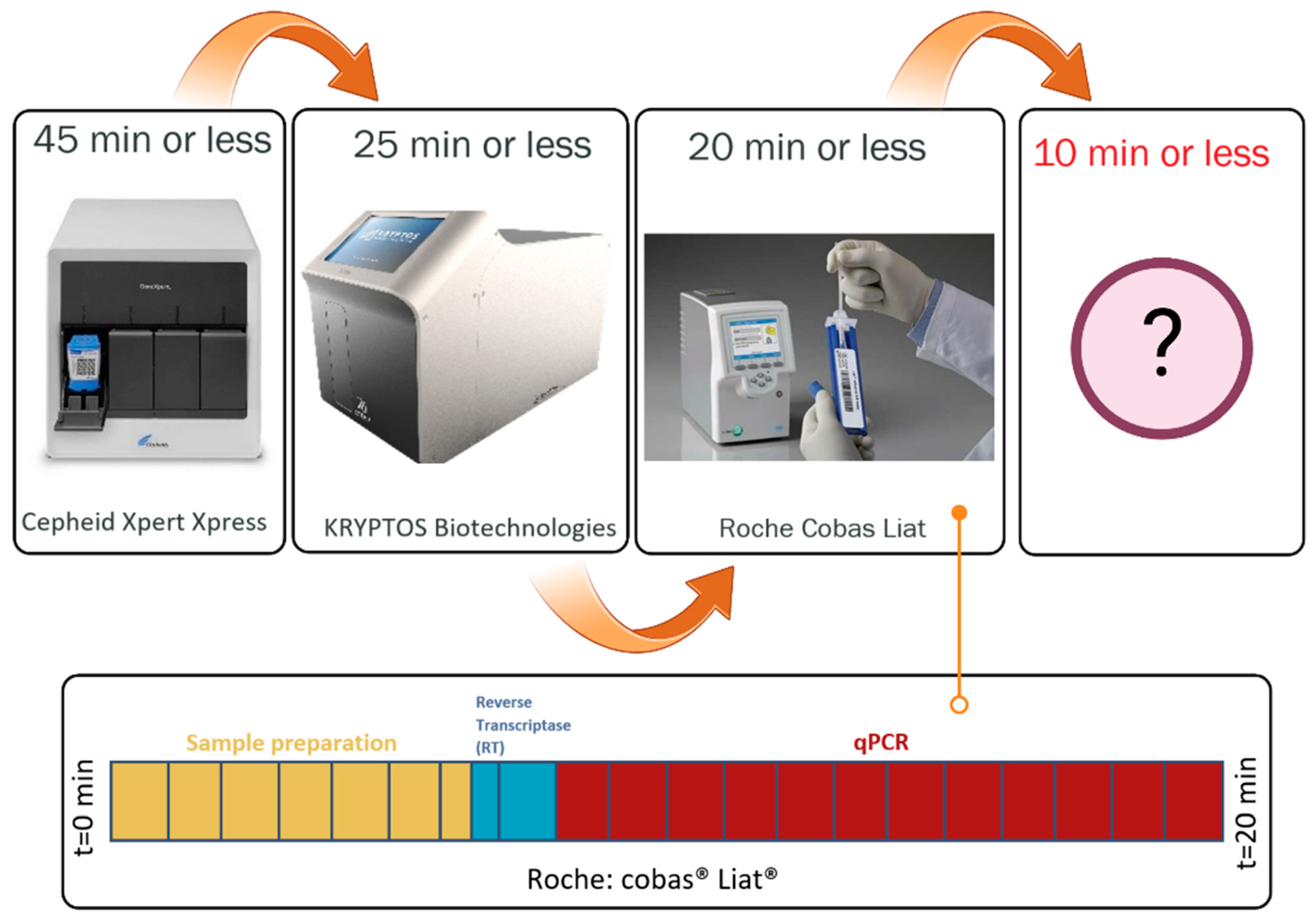
Figure 3.
Scaling of concentrations and sample volumes; (a) typical chemical and biological concentrations available for a few kinds of analysis. In general sample quantities in the picoliter to nanoliter range are sufficient for assaying the biological molecules involved in clinical chemistry assays (between 1014 and 1020 copies/mL) and immunoassays (between 107 and 1018 copies/mL). A minimum of 100 µL is required for accurate DNA assays (from 107 copies/mL to less than 100 copies/mL). (b) The probability that a given partition contains exactly k molecules for different values of λ.
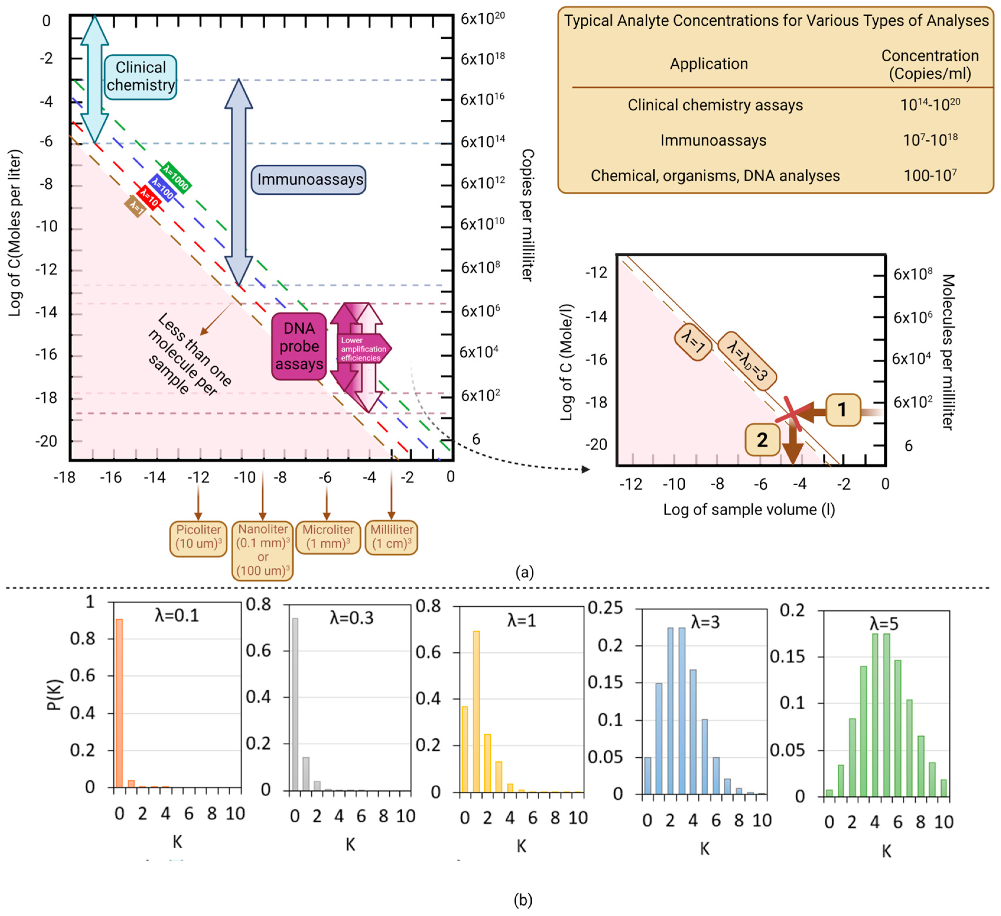
Figure 4.
Two typical PCR reactor configurations. (a) A ramping PCR system, where the temperature of both heaters on both sides of the reactor is ramped from 60 to 95 °C. (b) A shuttling PCR, where the reactor is shuttled from one temperature zone to another briefly exposing the reactor walls to air in between. τDNA is a time associated with the slowest reaction step in the amplification of DNA. τc is the time constant for the convection of air over the PCR reactor, is the heat diffusion time for water, is the heat diffusion time for the insulating reactor wall, and is the heat diffusion time for the heater.

Figure 5.
Simulation domains and contact resistance between the heater surface and insulator. Orange layers show a thin layer (thickness = 300 μm) of heater with a constant temperature of 95 °C; yellow layers show the insulator (thickness = 25 µm to 150 µm); and the blue layer shows the PCR solution considered as water (thickness = 100 µm to 500 µm). Only a thin layer (300 µm) of heater very close to the interface has been considered.
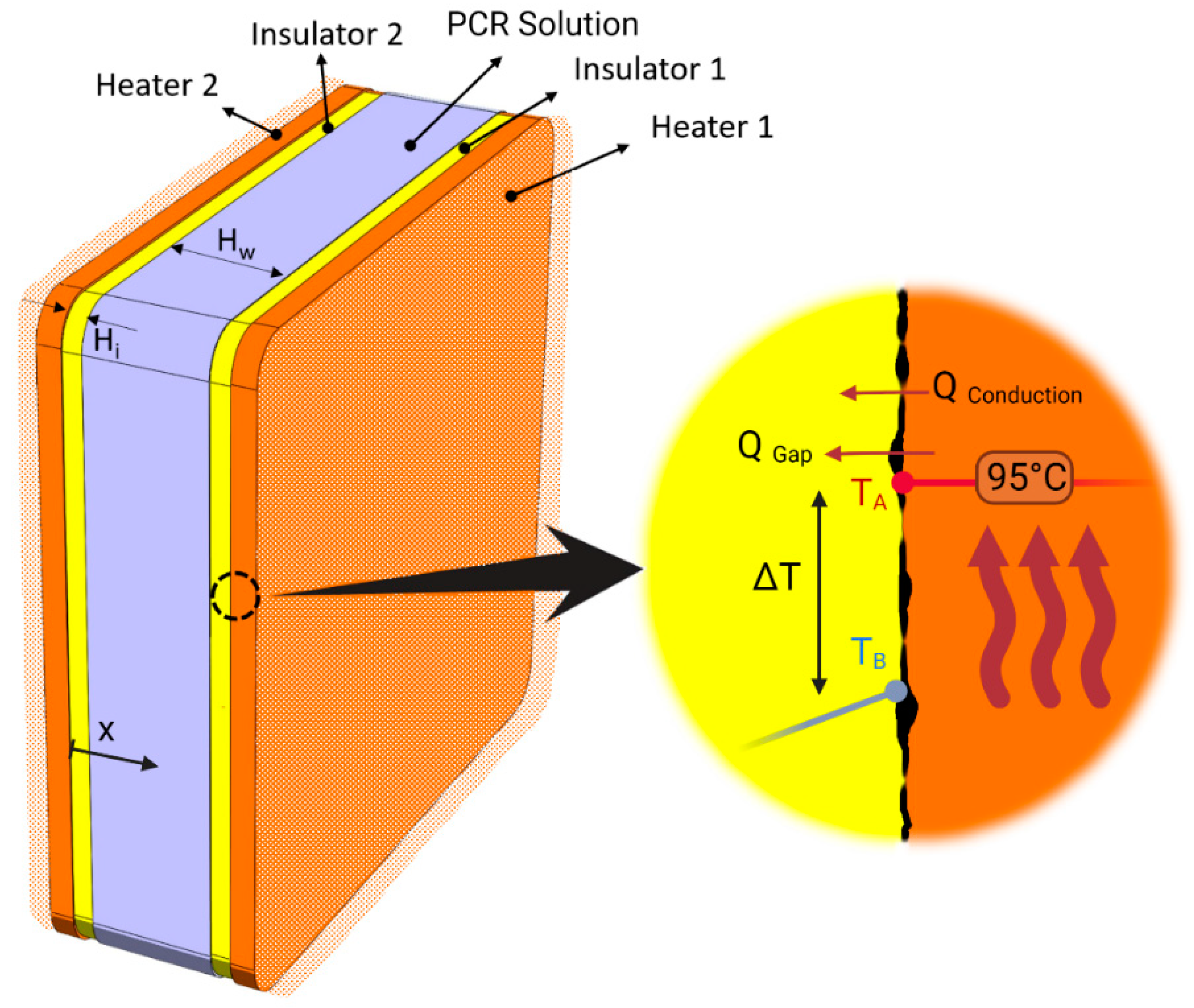
Figure 6.
(a) Effect of chamber height and contact resistance on temperature distribution over time. The solid vertical black lines mark the insulator-to-solution transition and the horizontal line at 93 °C marks the maximal allowed spread of reactor mix temperature (2 °C). (b) Ramping, cycle, and total times of different configurations of contact resistance and water heights.

Figure 7.
(a) Effect of insulator thickness on temperature distribution over time with the constant contact resistance of 2 K/W. The solid vertical black lines mark the insulator-to-solution transition and the horizontal line at 93 °C marks the maximal allowed spread of reactor mix temperature (2 °C). (b) Ramping, cycle, and total times of different configurations of insulator thickness and water heights.


Table 1.
Thermal characteristics of common materials used in PCR.
| Material | Thermal Conductivity (W/m·K) | Density (kg/m3) | Specific Thermal Capacity (kJ/kg K) | Thermal Diffusivity (m2/s) | Ref. | |
|---|---|---|---|---|---|---|
| Solids | PMMA | 0.21 | 1202.9 | 1.46 | 1.19 × 10⁻⁷ | [32] |
| PDMS | 0.15 | 970 | 1.46 | 1.06 × 10⁻⁷ | [33] | |
| PC | 0.2 | 1226.7 | 1.22 | 1.34 × 10⁻⁷ | [32] | |
| COC 8007 | Between 0.12 and 0.15 | 1020 | 1.2 | 1.17 × 10⁻⁷ | [34] | |
| PP | 0.22 | 900 | 1.330 to 2.400 | 0.961 × 10⁻⁷ | [35] | |
| Silicon | 148 (3.2 to 150) | 2330 | 0.712 | 9 × 10⁻⁵ | [36,37] | |
| Teflon | 0.35 | 2200 | 0.97 | 1.64 × 10⁻⁷ | [36] | |
| Glass | 1.4 | 2500 | 0.75 | 7.46 × 10⁻⁷ | [36] | |
| Liquid | Water | 0.613 | 997 | 4.17 | 1.47 × 10⁻⁷ | [36] |
| Oil | 0.131 | 837 | 1.67 | 7.85 × 10⁻⁸ | [36] |
Table 2.
Selected commercialized or under development PCR devices.
| Type of System | Device/Company | Time to Result | Characteristics | Thermal Contact Resistance | γ = Time/Volume |
|---|---|---|---|---|---|
| Plate system, not an integrated system, up to 96 wells |  NextGenPCR® MBS Molecular Biology Systems (Goes, The Netherlands) | 2 min without sample preparation |
| Low (squeezing pressure) | 2 min/20 µL = 0.1 |
| Integrated POC system | 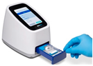 Lex Diagnostics (Melbourn, UK) | Sample to answer of 5 min and thermal cycling time of less than 3 min |
| Very low (engineered permanent contact) | 3 min/5 µL = 0.6 With heater on both sides: 3 min/10 µL = 0.3 |
| Plate system, not an integrated system, up to 96 wells |  XXPress BJS Technologies (Duluth, GA, USA) | 10 min without sample preparation |
| Lowest (engineered permanent contact) | 10 min/40 µL = 0.4 |
| Integrated POC system |  Roche’s Cobas Liat (Basel, Switzerland) | 20 min with sample preparation, 12 min for PCR |
| Low (squeezing pressure) | 12 min/80 µL = 0.15 |
Disclaimer/Publisher’s Note: The statements, opinions and data contained in all publications are solely those of the individual author(s) and contributor(s) and not of MDPI and/or the editor(s). MDPI and/or the editor(s) disclaim responsibility for any injury to people or property resulting from any ideas, methods, instructions or products referred to in the content. |
© 2023 by the authors. Licensee MDPI, Basel, Switzerland. This article is an open access article distributed under the terms and conditions of the Creative Commons Attribution (CC BY) license (https://creativecommons.org/licenses/by/4.0/).
Share and Cite
MDPI and ACS Style
Madadelahi, M.; Madou, M.J. Rational PCR Reactor Design in Microfluidics. Micromachines 2023, 14, 1533. https://doi.org/10.3390/mi14081533
AMA Style
Madadelahi M, Madou MJ. Rational PCR Reactor Design in Microfluidics. Micromachines. 2023; 14(8):1533. https://doi.org/10.3390/mi14081533
Chicago/Turabian StyleMadadelahi, Masoud, and Marc J. Madou. 2023. "Rational PCR Reactor Design in Microfluidics" Micromachines 14, no. 8: 1533. https://doi.org/10.3390/mi14081533
Note that from the first issue of 2016, this journal uses article numbers instead of page numbers. See further details here.