
Numerical Simulation of the Influence of Non-Uniform ζ Potential on Interfacial Flow


State Key Laboratory of Photon-Technology in Western China Energy, International Collaborative Center on Photoelectric Technology and Nano Functional Materials, Laboratory of Optoelectronic Technology of Shaanxi Province, Institute of Photonics & Photon Technology, Northwest University, Xi’an 710127, China
*
Author to whom correspondence should be addressed.
Micromachines 2024, 15(3), 419; https://doi.org/10.3390/mi15030419
Submission received: 9 February 2024
/
Revised: 18 March 2024
/
Accepted: 19 March 2024
/
Published: 21 March 2024
(This article belongs to the Section A:Physics)
Abstract
:Zeta potential (ζ potential) is a significant parameter to characterize the electric property of the electric double layer (EDL), which is important at the solid–liquid interface. Non-uniform ζ potential could be developed on a chemically uniform solid–liquid interface due to external flow. However, its influence on the flow has never been concerned. In this investigation, we numerically studied the influence of non-uniform 2D ζ potential on the flow at the solid–liquid interface. It is found, that even without any external electric field and only considering the influence of 2D ζ potential distribution, swirling flow can be generated near EDL, according to the rotational electric volume force. The streamwise vortices, which are important in the turbulent boundary layer, are theoretically predicted in this laminar flow model when considering the 2D distribution of ζ potential, implying the necessity of considering the origin of streamwise vortices of the turbulent boundary layer from the perspective of electrokinetic flow. In addition, the ζ potential distribution can promote the wall shear stress. Therefore, more attention must be paid to shear-sensitivity circumstances, like biomedical, medical devices, and in vivo. We hope that the current investigation can help us to better understand the effect of charge distribution on interfacial flow and provide theoretical guidance for the development of related applications in the future.
1. Introduction
Electric double layer (EDL) is a kind of physical structure that exists generally in the two-phase interface or even three-phase interface (including solid, liquid, and gas). Taking the solid–liquid interface as an example, when the electrolyte solution flows through the channel, charges will be redistributed on the channel wall. Under the influence of the surface charge, ions in the solution with the opposite charge of the surface charge, i.e., counter-ions, will gather on the surface of the solid, causing the corresponding positive or negative charges to be reordered. Two thin layers with different electric properties can be formed on the interface, including a Stern layer and diffuse layer, constituting the important and common interface electric structure—EDL.
Due to the widespread existence of interfacial phenomena [1,2,3,4,5], EDL and its dynamics play important roles in many fields, such as microfluidic technology [6,7,8], electrochemical analysis [9], energy systems [10,11], and biomedical applications (e.g., pharmaceutical analysis [12] and cell detection [13]). Relying on the electric properties of EDL, the electrokinetic (EK) flow (like electroosmotic flow) under the action of electric field have been broadly applied, to control flow [14], deliver drugs [15], enhance mixing in micro-/nanofluidic devices [16,17], etc. EDL also occupies a central position in solving many global problems (e.g., water desalination [18], sewage treatment [19], etc.).
The Gouy–Chapman–Stern–Grahame (GCSG) model is a widely accepted EDL model, which holds that EDL is composed of a Stern layer and a diffuse layer [20,21,22,23]. The ions in the Stern layer are considered to be adsorbed and fixed on the solid surface, while the ions in the diffuse layer but near the Stern layer cannot move freely due to the strong electrostatic force locally. As the distance from the Stern layer is beyond a certain level, the electrostatic force is not enough to restrain the thermal motion of the ions, and the ions diffuse randomly in the solution, which also shows that the diffuse layer as a dynamic structure can slide on the charged surface. The position where the ions are ready to move is called the shear plane. The ζ potential is the potential at the shear plane [23].
The ζ potential is a key parameter to characterize the electric structure in EDL. It plays an important role in interface science (e.g., interfacial reaction [24,25], self-assembly [26,27], etc.) and electrokinetic flow dynamics [28,29,30]. However, limited by electrochemical analysis techniques [31,32,33,34] on ζ potential, the hypothesis of chemically uniform interfaces with unique ζ potential was usually considered in past research. Our understanding of local ζ potential and its influence on diverse disciplines is nearly blank.
In recent years, with the in-depth study of nanoscale interface phenomena and the development of new materials with complex surfaces and superstructures, researchers have gradually begun to pay attention to the influence of non-uniform surface charge on the electrical properties of the interface and explore the factors affecting the surface charge distribution and the corresponding potential.
On one hand, relevant research shows that chemically homogeneous slab channel walls exhibit non-uniform ζ potential under the action of an outflow field. For example, Lis et al. [35] using vibrational sum frequency generation (v-SFG) spectroscopy preliminarily reveal that surface potentials vary with external flows temporally. Subsequently, Werkhoven et al. [36] showed theoretically that a pressure-driven flow can induce a strong heterogeneous surface charge and ζ potential on a chemically homogeneous channel wall. Ober et al. [37] show that liquid flow along the surface of CaF2 creates a reversible space charge gradient by v-SFG spectroscopy as well. In a current investigation, relying on a novel fluorescence photobleaching electrochemistry analyzer (FLEA), Meng et al. [38] reported a two-dimensional ζ potential induced by external flow at the solid–liquid interface.
On the other hand, non-uniform ζ potential can lead to unpredicted outcomes in diverse fields. Paratore et al. [39] demonstrated that the flow that surrounds a surface with non-uniform surface charge density (ζ potential as well) can induce complex flow patterns without a physical constraint. Yang et al. [40] revealed that gold superlattices with nanoscale variations in ζ potential distribution can significantly augment electrochemical reactions, underscoring the profound impact of ζ potential heterogeneity on electrochemical processes.
In the investigation, according to the previous experimental and theoretical reports, we hope to show how the non-uniform ζ potential distribution influences the electric volume force and its influence on the flow, through the numerical simulation method.
2. Theory
The momentum transport process of EK flow can be described by the Navier–Stokes equation with the electric volume force term, which is expressed as:
where is the fluid density, is the pressure on the fluid, is the dynamic viscosity. is the velocity vector, with , and being the velocity components in , , and directions, respectively, and , and the corresponding unit vectors in Cartesian coordinates (see Figure 1). is the electric volume force (EVF), which can be expressed as [41,42,43].
where is electric charge density, is the vector of electric field strength. In homogeneous dielectric media with incompressible approximation, the variation of is ignored, thus , with and being:
where is the electric potential in the EDL, is electric permittivity with being the vacuum permittivity, and is the relative permittivity of fluid. When the potential changes slowly, the potential distribution in the EDL can be approximately described by Poisson–Boltzmann theory as:
where is the Boltzmann constant, is temperature, is the elementary charge, and is the relative valence state of ions in electrolytes. is the Debye length, which is a characteristic length of the EDL. is Avogadro constant, and is the concentration of ions in electrolytes.
Under steady state, divide both sides of Equation (1) by , and then calculate the curl on both sides with incompressible fluid relation. Thus,, we have:
where is the vorticity, is the kinematic viscosity coefficient, and is the driving term of vorticity equation. According to Maxwell’s equations and assuming the magnetic field is steady, by substituting Equations (3) and (4) into , we find
For convenience, let , , (with are either 1 or 2), from Equation (5), it is obtained
and
where , , , , and is thermal potential. Furthermore, after substituting Equations (8)–(10) into and , we have
and
It can be seen when is non-uniform in 2D, , , and can be non-zero. All the three components in Equation (12) can be nonzero, and thus, the driving term of vorticity is:
Therefore, based on Equation (6), the electric volume force with curl can drive the fluid to produce a swirling flow. It is worth noting that, since there is no external electric field applied, we only consider the Coulomb force in Equation (1). The influence of other electric volume forces, e.g., according to electrothermal or dielectric effect, are believed to be absent in this investigation.
3. Numerical Simulation
Based on the theory above, we can make a reasonable prediction that in the steady-state flow field, such as pressure-driven flow, there may be a non-uniform two-dimensional ζ potential distribution at the solid–liquid interface, which will induce the generation of local electrostatic charge and EVF, resulting in a swirling flow near the interface. To validate this conjecture, we established a mathematical model of non-uniform ζ potential distribution and proceeded with a numerical simulation by Comsol Multiphysics on Equations (1)–(5). The influence of non-uniform ζ potential distribution at the solid–liquid interface on the flow is investigated under steady-state approximation with the value of relative tolerance is .
3.1. Pressure-Driven Laminar Flow
In this simulation model, the material is liquid water, with electric conductivity and pH values are μS/cm and , respectively. The thickness of the EDL on the bottom of the microchannel, i.e., Debye length, is estimated to be 11 nm. The specific physical parameters are shown in Table 1.
The basic flow is a pressure-driven steady flow with incompressible conditions. The bulk flow Reynolds number , indicating the basic flow is a typical laminar flow. Here, is the hydraulic diameter of the flow, is the bulk flow velocity, is flow rate, and is the cross-sectional area of the computational regime.
In the laminar flow interface, the two sides of the rectangular model that are perpendicular to the direction are set to the inlet and outlet, respectively. At the entrance, the fully developed flow condition has been applied, with the average velocity m/s. At the exit, the boundary condition is suppressing backflow (which adjusts the outlet pressure to reduce the amount of fluid entering the domain through the exit), with static pressure Pa. According to the symmetry of the geometric model and the rationality of the physical model, a no slip boundary condition has been imposed on the other four walls (including the upper wall, bottom wall, and two side walls), where the fluid velocity is zero. Electric volume force has been applied to the entire domain of the model (see Equation (5), similar to potential , and is dominant in the EDL at the bottom of microchannel), as shown in Figure 1.
3.2. Electrostatics Module
In this investigation, there is no external electric field applied, and the electric volume force is entirely generated by the 2D distribution of ζ potential. To study the effect of the electrical volume force due to the non-uniform ζ potential on the flow field, the electrostatic interface has been added into the simulation model. Furthermore, since the electric field is steady, the effect of the magnetic field is negligible.
The charge is conserved throughout the domain, and the electroosmotic potential calculated by Equation (5) was applied in the entire physical model. To further reduce the computational cost, we calculate the electric volume force by defining custom variables and analytic functions according to Equations (2)–(5).
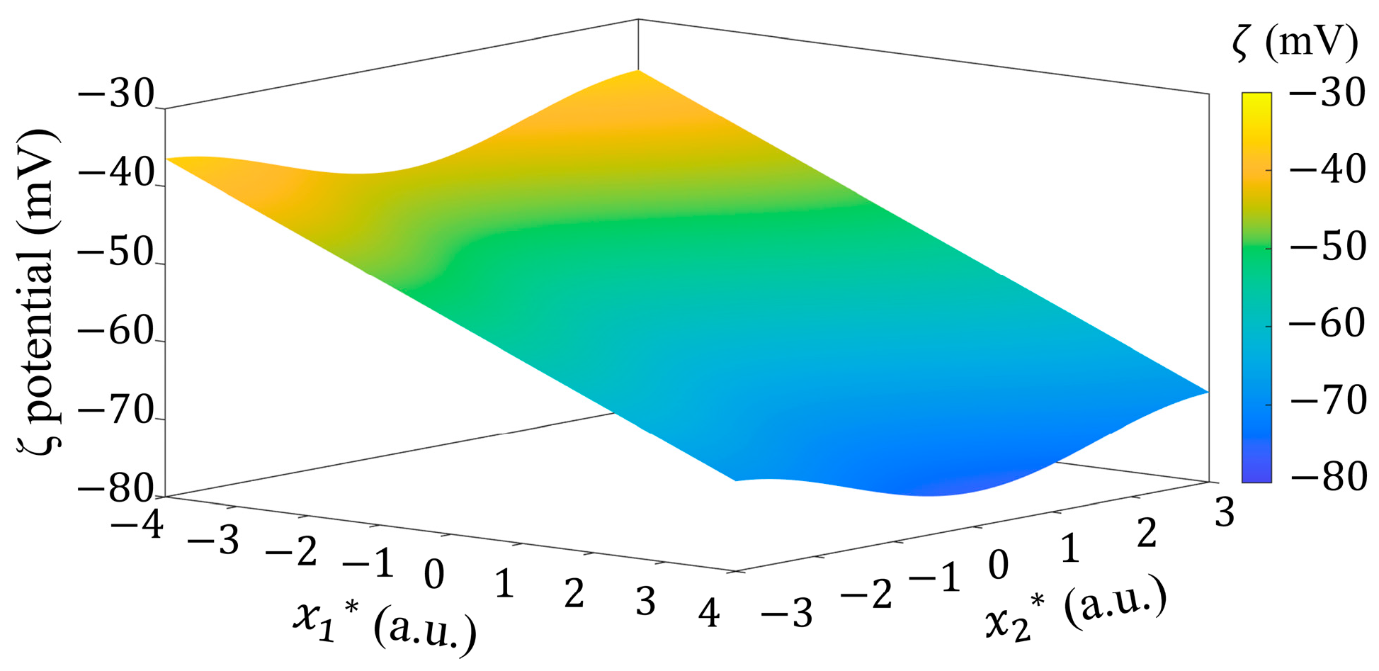
As mentioned above, in order to investigate the effect of non-uniform ζ potential distribution on interfacial flow, a mathematical model of ζ potential distribution (as plotted in Figure 2) was established to characterize the ζ potential distribution in the solid–liquid interface at the bottom of the microchannel only (as shown in Figure 1) based on the recent report of Meng et al. [38], as
where is the classical ζ potential value at the interface of water-fused silica [44]. The slope represents how quickly the ζ potential increases in the streamwise direction (with ). The dimensionless amplitude represents the variation of ζ potential along the spanwise direction. The wavenumber determines the possible periodicity of ζ potential in the spanwise direction.
By substituting Equation (14) into Equation (5), electroosmotic potential could be calculated. In turn, the electric charge density , electric field strength , EVF, and could be calculated accordingly by Equations (3), (4), (11) and (12).
Finally, it is worth noting that due to the choice of steady-state study method, initial values of velocity, pressure, and potential are not considered when the boundary conditions are set.
3.3. Modeling and Meshing
The computational regime is a cuboid with dimensions in the order of micrometers. In the - plane, the geometric model is built around the origin . In the investigation, the potential (see Equation (5)) decreases exponentially with and is dominant only in the EDL at the solid–liquid interface. To capture the influence on flow dynamics, grid cells with nanoscale resolution are required. However, to be able to capture the evolution of flow, a large computational domain is required. To compromise these two requirements, the computation regime is μm long, μm wide, and μm high. Thus, we can capture the influence of micrometer variation of ζ potential on the flow. In the modeling process, the geometric model is divided into three regions in the direction, including a large bulk region ( μm) in the center of the channel and two symmetrical thin-layer regions ( nm) near the bottom and upper wall.
In the meshing process, mapping operation is used in the - plane, and sweeping operation is carried out upward from the bottom to the upper wall in the direction and downward from the ceiling to the under wall in the opposite of the direction, respectively, in the two thin-layer regions. The grid can be denser in the target area by the arrangement of geometric sequence. Detailed grid distribution of each region is shown in Figure 3.
During the sweeping operation in the direction, the grid in the thin-layer region is divided down to the nanometer scale to ensure resolution. The minimum and maximum grid sizes are 1.33 nm and 2.66 nm, respectively. While in the bulk region, the grid is much coarser with a fixed size of 180 nm. In the - plane, both bulk region and thin-layer region have the same minimum grid size and the same maximum grid size. In the direction, the minimum and maximum grid sizes are 6.68 nm and 20 nm, respectively. In the direction, the minimum and maximum grid sizes are 4.42 nm and 13.26 nm, respectively. Hexahedral grid elements are used for all regions in the model. Detailed parameters for complete grid statistics of the model are shown in Table 2.
3.4. Grid Independence Analysis
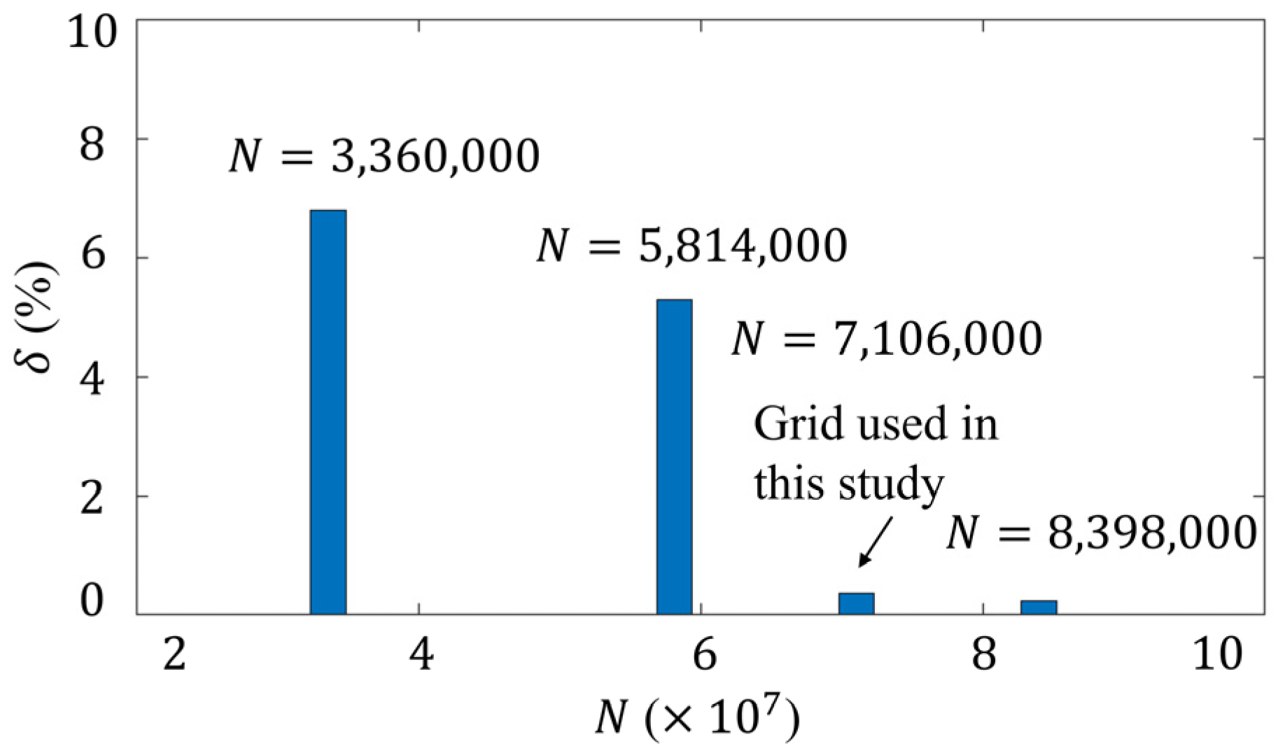
To ensure computational validity and stability, we conducted a grid independence analysis by systematically varying the grid size in all dimensions while keeping other parameters such as boundary conditions and solvers unchanged. The relative errors () of the simulated velocity field between the models of different grid quantities () are plotted in Figure 4. It can be seen that decreases asymptotically towards zero, with the increase in grid quantity. The minimum value is 0.24%. The results show that when the grid quantity is equal to or beyond , is within 1%, indicating a negligible dependency of computational results on grid density [45]. Consequently, to strike a balance between computational efficiency and precision, we adopted a grid resolution of for subsequent analyses in this study.
4. Results
4.1. Pressure-Driven Basic Flow
In the previous investigations on interfacial flow, the influence of interfacial charge distribution and potential distribution was not taken into account. The basic flow (e.g., common Poiseuille flow) is driven only by pressure.
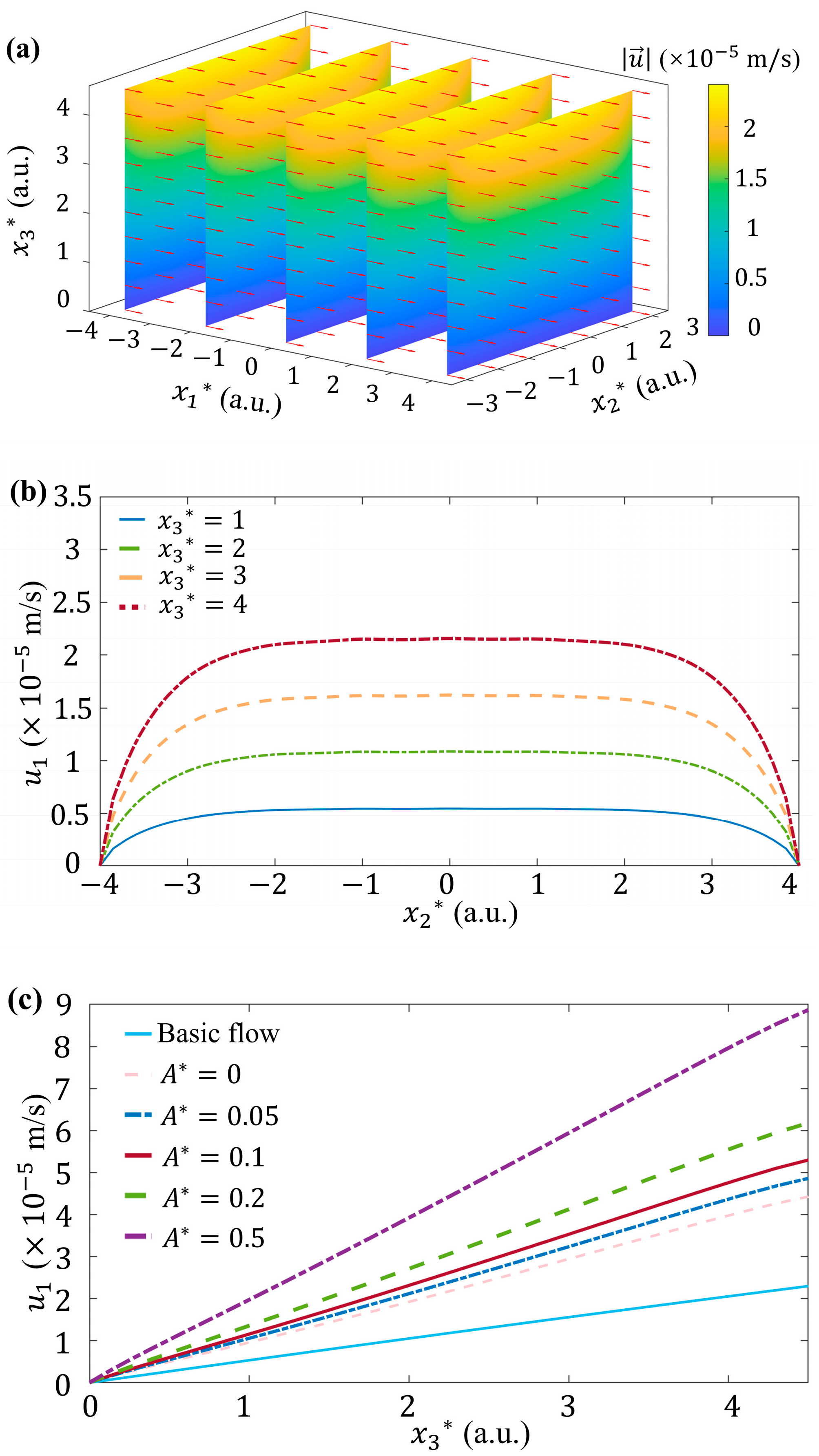
In this case, the velocity field distribution of the basic flow is shown in Figure 5a, where , , with characteristic length μm and Debye length nm. We applied a small volume rate (), where the basic flow velocity is m/s at 0.5 µm from the wall, to simulate a relatively large wall strain rate (240 s−1). Slice and quiver diagrams are used to show the distribution of the intensity (where the magnitude of intensity is represented by the color) and direction of the fluid velocity in the - planes at different streamwise positions. The direction of the fluid velocity after normalization at each position is represented by the vector arrow. Due to the absence of the external force, the velocity of the basic flow shows an approximately parabolic distribution in the spanwise direction near the wall, as can be found in Figure 5b with .
In contrast, as shown in Figure 5c, since the EDL is extremely thin, the streamwise component of velocity, i.e., , shows a linear variation with the dimensionless vertical position . This is an approximation of the parabolic velocity distribution of Poiseuille flow in the thin EDL.
4.2. Uniform ζ Distribution
When considering the presence of uniformly distributed ζ potential (i.e., ) at the solid–liquid interface, based on Equation (5), it can be seen that there is an electroosmotic potential distribution in Figure 6a. It shows a uniform distribution in the - plane and exponential decay in the vertical direction. Accordingly, are all in the negative direction with decreasing magnitudes from bottom to top, as shown in Figure 6b. is exactly zero everywhere. In other words, the uniform distribution of the ζ potential induces irrotational . Under the influence of , the velocity distribution of the flow field is shown in Figure 6c. Compared with Figure 5a, it is obvious that the direction of the velocity has not changed, which still dominated by the -directional component . Furthermore, the parabolic velocity distribution in the and directions are still present.
From the perspective of vortex dynamics, the source term in Equation (6) does not exist in either the basic flow or the flow field considering uniform ζ potential. Therefore, it does not disturb the basic flow, nor drive the fluid to produce vorticity, and cannot cause the vorticity to deform (stretch, tilt, twist, etc.).
4.3. One-Dimensional ζ Distribution
In this subsection, we consider if an 1D distribution of ζ potential with a certain slope in the x direction is formed due to nonuniform interface charge redistribution by the basic flow. Let in Equation (14), we have:
Taking 1/m and mV as an example, the 1D distribution of ζ potential see Figure 7a, and the distributions of and induced by this ζ potential are shown in Figure 7b and Figure 7c, respectively. Based on the increase in in the direction, the strength of also shows an increasing trend from upstream to downstream. Compared with Figure 6b, although the component of is still dominant, the component of the is not zero anymore. This subsequently means that the component of , i.e., , as shown in Figure 7c.
Although the flow with 1D ζ potential distribution can induce the electric volume force with and , in this case, we still have the streamwise and vertical components of , i.e., which could be seen more intuitively in Figure 7d. According to Equation (6), . There is no vorticity generated in streamwise and vertical directions through the electrical volume force, except for and . As a result, the velocity distribution of the flow field in Figure 7e shows a clear difference from Figure 5a and Figure 6c. The dominancy of is no longer always true; in contrast, becomes dominant when . Compared with the basic flow, both (Figure 5c) and have exhibited significant increment. The parabolic distribution in the direction of basic flow (see Figure 5b) is no longer present when considering 1D ζ potential distribution.
4.4. Two-Dimensional ζ Distribution
In this subsection, the influence of the 2D distribution of ζ potential on flow is investigated. In Equation (14), we take 1/m, , mV, and as an example. The ζ potential exhibits a 2D distribution on a solid–fluid surface, as plotted in Figure 2.
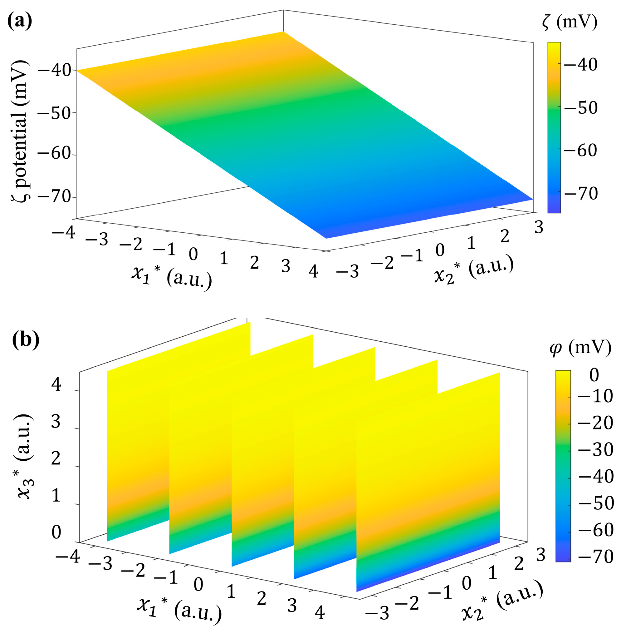
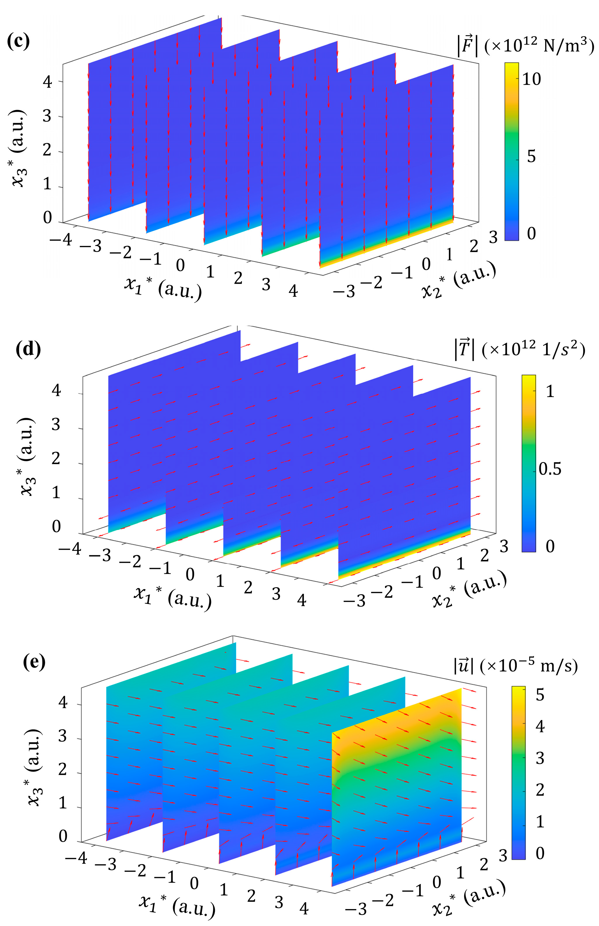
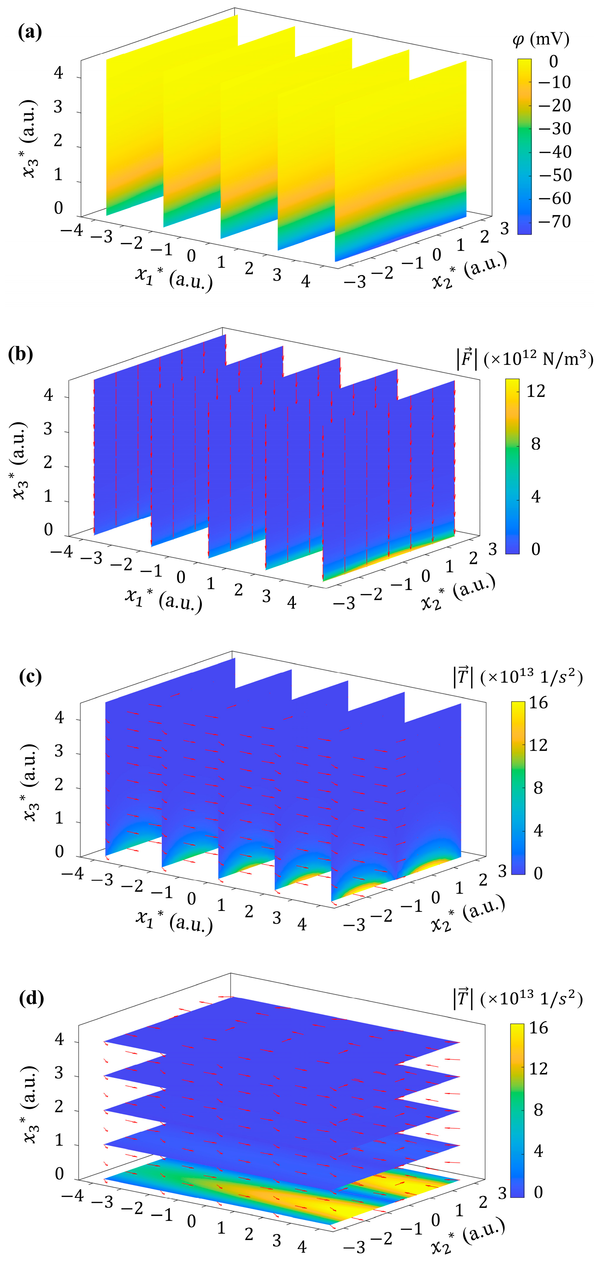
Based on Equations (2)–(5), a 3D electroosmotic potential distribution is generated in the EDL at the bottom of the microchannel (as shown in Figure 8a), which in turn generates local electric charge and induces a non-uniform electric volume force. As shown in Figure 8b, exhibits strong -directional component. The directions of are mainly pointing to the bottom wall of the microchannel. The strength of generally shows a decaying trend along , reaching a maximum at one Debye length above the bottom wall. The strength of also exhibits variations along the streamwise direction and the spanwise direction. It increases gradually downstream and decreases from the center of the flow field, forming an approximate symmetry distribution along the spanwise direction.
Different from the induced by 0D (Figure 6b) and 1D (Figure 7c) distributions of ζ potential, in the model of 2D ζ potential, can be rotational in 3D. All three components of can be non-zero, as shown in Figure 8c,d. increases in the streamwise direction, which is consistent with that of . In the spanwise, shows an approximate symmetry with respect to the center of the channel, but in opposite directions (see Figure 8d). Two maxima can be observed at −1.5 and 1.5.
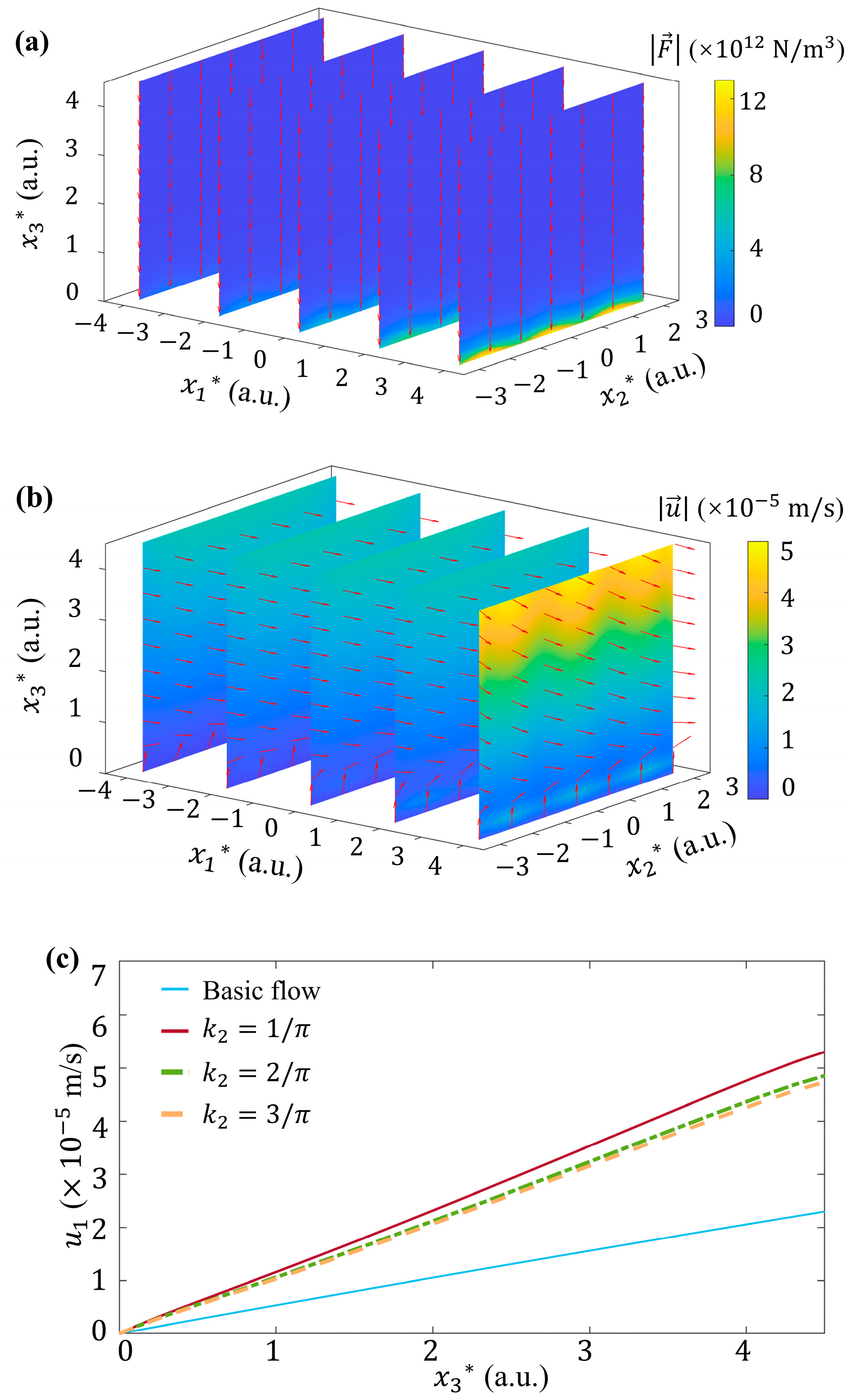
The fluid velocity distribution under the driven of rotational is shown in Figure 9a. The vertical velocity component was observed near the bottom within one Debye length (i.e., ). While component begins to dominate at . This phenomenon suggests that even though most of the electric volume force is offset by pressure gradient, such a large volume force will still have a significant impact on the velocity field. At the height of and higher, is concentrated in the center of the microchannel in the spanwise to reach the maximum, which shows significant difference from those in Figure 5a, Figure 6c and Figure 7e.
In order to further explore the influence of 2D ζ potential on the interfacial flow, the velocity distribution in the - plane that one Debye length from the bottom () is shown in Figure 9b by a surface diagram. It can be seen that the velocity of the flow, considering the effect of caused by 2D ζ potential distribution, is about 3 folds higher than the basic flow. It exhibits an obvious increasing trend from upstream to downstream in the streamwise direction. In this plane, , rather than , is dominant among the three components of the flow velocity, indicating that the electric volume force (after being mostly balanced by the pressure term of Equation (1)) can cause the development of flow at the bottom wall. This implies, when considering the EK flow driven by 2D ζ potential, the momentum transport near the interface can be significantly promoted.
The non-zero further generates in the flow field, as shown in Figure 9c. Particularly, the streamwise component of vorticity is non-zero, i.e., , and is gradually strengthened from upstream to downstream. In the upstream region, mainly aligns along the direction with approximately uniform distribution on the same . While in the downstream, this distribution is broken. becomes bending towards the streamwise direction, indicating the possible generation of streamwise vortices.
Streamwise vortices commonly exist in flow boundary layers, e.g., the well-known coherent vortex structures in the turbulent boundary layer. However, the origin of such vortices remains unclear. We hope to give an insight into this problem through the vision of electrokinetic mechanism, and provide a new approach to control the generation and evolution of vortices in boundary layers.
5. Discussion
In this section, the influence of the parameters (such as slope , dimensionless amplitude , initial zeta potential , and wavenumber ) on the flow are systematically investigated by numerical simulations.
5.1. Influence of
In this subsection, the influence of slope on the flow is investigated at , mV, and . In Figure 10a, it is obvious that shows a linear increment with , which is an approximation of the parabolic distribution caused by fluid viscosity in a thin layer. When the slope gradually increases, a stronger variation of ζ potential along the streamwise direction is induced. The streamwise component of electric volume force gradually increases as well (see Figure 10b), accompanied by the increasing and velocity gradient . Thus, the wall shear stress is:
which considering 2D ζ potential distribution can be significantly stronger than that of basic flow, as can be seen more clearly in Figure 10c.
5.2. Influence of
The influence of is investigated at 1/m, mV and , as shown in Figure 5c. The comparison between the basic flow and the flow under 1D ζ potential (i.e., ) shows that the fluid velocity can be enhanced even if . When spanwise variation of ζ is taken into account, both and velocity gradient are strengthened at larger , indicating stronger wall shear stress as well.
5.3. Influence of
5.4. Influence of
At last, we discuss the influence of spanwise distributions of ζ potential on the flow, under 1/m, , and mV. Larger indicates a wavier distribution of ζ potential in the direction, which induces a stronger gradient of ζ potential and more peak value positions of as well. At as an example, the electric volume force and the corresponding fluid velocity both exhibit wavy distribution along the spanwise direction, as shown in Figure 12a,b. Even if the peak values of at are equal to that of shown in Figure 8b, the peak value of becomes decreased a little bit relative to Figure 9a. The increasing also decreases the streamwise velocity and its gradient (Figure 12c). Therefore, a smaller of flow can be concluded.
All in all, it can be seen, when taking the influence of 2D ζ potential into account, the wall shear stress can be significantly enhanced. For example, at 1/m, , mV, and , the maximum can be up to Pa, which is about 2.5 folds larger than the basic flow. A stronger wall shear stress indicates a stronger interaction between wall and flow. This could be important in many shear-sensitive circumstances, especially on biological materials. One example is that the flow shear stress on cells and tissues may be larger than previously expected. Studying the different control parameters of 2D potential distribution can help us better understand the effect of charge distribution on interfacial flow, and according to Equation (16), we can even realize of adjustment of wall shear stress by changing these parameters.
5.5. Influence of Other Parameters
In addition to the parameters of the zeta potential distribution discussed above, there are also several other parameters that affect the EK flow at the solid–liquid interface, for example, the electric conductivity and viscosity of the fluid. On the one hand, the electric conductivity is closely related to Debye length, which affects the distribution of electric potential and charge density in the EDL. This in turn affects electric volume force and the flow as delineated in Equations (2)–(5). On the other hand, the influence of viscosity is also important. The EK flow induced by non-uniform ζ potential is intrinsically a balance between EVF and viscosity [46,47], primarily due to the balance of electric volume force and the viscous effect. The changing of viscosity could affect both the velocity profile and wall shear stress near the wall. However, a comprehensive exploration on these parameters accompanied with zeta potential variation are beyond the scope of this manuscript and will be studied in future works.
6. Conclusions
In this investigation, the influence of the non-uniform 2D distribution of ζ potential on the flow at the solid–liquid interface has been investigated numerically. Since the electric volume force can be rotational, it further drives the fluid to produce a swirling flow. The streamwise vortices, which are important in the turbulent boundary layer, are theoretically predicted in this laminar flow model when considering the 2D distribution of ζ potential. This observation implies it is necessary to reconsider the origin of streamwise vortices in turbulent boundary layer, from the perspective of electrokinetic flow. In addition, when considering the influence of ζ potential distribution, the wall shear stress can be apparently larger relative to no ζ potential considered. This is important for shear-sensitivity circumstances, particularly in biomedical and medical devices, and in vivo. We hope the present work provides a theoretical foundation to understand the complex development and evolution mechanism through various electrical and dynamics parameters, and provides a new way to control the vortices and shear stress in boundary layers.
Author Contributions
Conceptualization, W.Z.; methodology, Y.H.; software, Y.H.; validation, W.Z.; formal analysis, Y.H. and W.Z.; investigation, Y.H.; resources, W.Z.; data curation, Y.H.; writing—original draft preparation, Y.H.; writing—review and editing, W.Z.; visualization, Y.H.; supervision, W.Z.; project administration, W.Z.; funding acquisition, W.Z. All authors have read and agreed to the published version of the manuscript.
Funding
This research was funded by National Natural Science Foundation of China, grant number 51927804.
Data Availability Statement
The original contributions presented in the study are included in the article, further inquiries can be directed to the corresponding author.
Conflicts of Interest
The authors declare no conflicts of interest.
References
- Toney, M.F.; Howard, J.N.; Richer, J.; Borges, G.L.; Gordon, J.G.; Melroy, O.R.; Wiesler, D.G.; Yee, D.; Sorensen, L.B. Voltage-dependent ordering of water molecules at an electrode–electrolyte interface. Nature 1994, 368, 444–446. [Google Scholar] [CrossRef]
- Bazant, M.Z.; Squires, T.M. Induced-Charge Electrokinetic Phenomena: Theory and Microfluidic Applications. Phys. Rev. Lett. 2004, 92, 066101. [Google Scholar] [CrossRef]
- Davidson, S.M.; Andersen, M.B.; Mani, A. Chaotic Induced-Charge Electro-Osmosis. Phys. Rev. Lett. 2014, 112, 128302. [Google Scholar] [CrossRef]
- Fernández-Mateo, R.; Calero, V.; Morgan, H.; Ramos, A.; García-Sánchez, P. Concentration–Polarization Electroosmosis near Insulating Constrictions within Microfluidic Channels. Anal. Chem. 2021, 93, 14667–14674. [Google Scholar] [CrossRef]
- Sparreboom, W.; Berg, A.v.d.; Eijkel, J.C.T. Principles and applications of nanofluidic transport. Nat. Nanotechnol. 2009, 4, 713–720. [Google Scholar] [CrossRef]
- Whitesides, G.M. The origins and the future of microfluidics. Nature 2006, 442, 368–373. [Google Scholar] [CrossRef] [PubMed]
- Wu, Y.; Ma, X.; Li, K.; Yue, Y.; Zhang, Z.; Meng, Y.; Wang, S. Bipolar Electrode-based Sheath-Less Focusing and Continuous Acoustic Sorting of Particles and Cells in an Integrated Microfluidic Device. Anal. Chem. 2024, 96, 3627–3635. [Google Scholar] [CrossRef] [PubMed]
- Wu, Y.; Zhang, H.; Yue, Y.; Wang, S.; Meng, Y. Controllable and Scaffold-Free Formation of 3D Multicellular Architectures Using a Bipolar Electrode Array. Adv. Mater. Technol. 2024, 9, 2301626. [Google Scholar] [CrossRef]
- Escosura-Muñiz, A.d.l.; Ambrosi, A.; Merkoçi, A. Electrochemical analysis with nanoparticle-based biosystems. TrAC Trends Anal. Chem. 2008, 27, 568–584. [Google Scholar] [CrossRef]
- Karden, E.; Ploumen, S.; Fricke, B.; Miller, T.; Snyder, K. Energy storage devices for future hybrid electric vehicles. J. Power Sources 2007, 168, 2–11. [Google Scholar] [CrossRef]
- Hu, Y.; Yang, J.; Hu, J.; Wang, J.; Liang, S.; Hou, H.; Wu, X.; Liu, B.; Yu, W.; He, X.; et al. Synthesis of Nanostructured PbO@C Composite Derived from Spent Lead-Acid Battery for Next-Generation Lead-Carbon Battery. Adv. Funct. Mater. 2018, 28, 1705294. [Google Scholar] [CrossRef]
- Cui, P.; Wang, S. Application of microfluidic chip technology in pharmaceutical analysis: A review. J. Pharm. Anal. 2019, 9, 238–247. [Google Scholar] [CrossRef]
- Wu, Y.; Gu, Q.; Wang, Z.; Tian, Z.; Wang, Z.; Liu, W.; Han, J.; Liu, S. Electrochemiluminescence Analysis of Multiple Glycans on Single Living Cell with a Closed Bipolar Electrode Array Chip. Anal. Chem. 2024, 96, 2165–2172. [Google Scholar] [CrossRef]
- Tiflidis, C.; Westerbeek, E.Y.; Jorissen, K.F.A.; Olthuis, W.; Eijkel, J.C.T.; Malsche, W.D. Inducing AC-electroosmotic flow using electric field manipulation with insulators. Lab Chip 2021, 21, 3105–3111. [Google Scholar] [CrossRef]
- Pikal, M.J. The role of electroosmotic flow in transdermal iontophoresis. Adv. Drug Deliv. Rev. 2001, 46, 281–305. [Google Scholar] [CrossRef] [PubMed]
- Wu, M.; Gao, Y.; Ghaznavi, A.; Zhao, W.; Xu, J. AC electroosmosis micromixing on a lab-on-a-foil electric microfluidic device. Sens. Actuators B 2022, 359, 131611. [Google Scholar] [CrossRef]
- Kneller, A.R.; Haywood, D.G.; Jacobson, S.C. AC Electroosmotic Pumping in Nanofluidic Funnels. Anal. Chem. 2016, 88, 6390–6394. [Google Scholar] [CrossRef] [PubMed]
- Porada, S.; Weinstein, L.; Dash, R.; Wal, A.v.d.; Bryjak, M.; Gogotsi, Y.; Biesheuvel, P.M. Water Desalination Using Capacitive Deionization with Microporous Carbon Electrodes. ACS Appl. Mater. Interfaces 2012, 4, 1194–1199. [Google Scholar] [CrossRef]
- Wang, C.; Gao, Q. 3D Numerical Study of the Electrokinetic Motion of a Microparticle Adsorbed at a Horizontal Oil/Water Interface in an Infinite Domain. ACS Omega 2022, 7, 4062–4070. [Google Scholar] [CrossRef] [PubMed]
- Santiago, J.G. Electroosmotic Flows in Microchannels with Finite Inertial and Pressure Forces. Anal. Chem. 2001, 73, 2353–2365. [Google Scholar] [CrossRef]
- Schoch, R.B.; Lintel, H.v.; Renaud, P. Effect of the surface charge on ion transport through nanoslits. Phys. Fluids 2005, 17, 100604. [Google Scholar] [CrossRef]
- Brown, M.A.; Abbas, Z.; Kleibert, A.; Green, R.G.; Goel, A.; May, S.; Squires, T.M. Determination of Surface Potential and Electrical Double-Layer Structure at the Aqueous Electrolyte-Nanoparticle Interface. Phys. Rev. X 2016, 6, 011007. [Google Scholar] [CrossRef]
- Saha, P.; Zenyuk, I.V. Electrokinetic Streaming Current Method to Probe Polycrystalline Gold Electrode-Electrolyte Interface Under Applied Potentials. J. Electrochem. Soc. 2021, 168, 046511. [Google Scholar] [CrossRef]
- Putnis, C.V.; Ruiz-Agudo, E. The Mineral–Water Interface: Where Minerals React with the Environment. Elements 2013, 9, 177–182. [Google Scholar] [CrossRef]
- Schaefer, J.; Gonella, G.; Bonn, M.; Backus, E.H.G. Surface-specific vibrational spectroscopy of the water/silica interface: Screening and interference. Phys. Chem. Chem. Phys. 2017, 19, 16875–16880. [Google Scholar] [CrossRef]
- Zhang, S.; Chen, J.; Liu, J.; Pyles, H.; Baker, D.; Chen, C.-L.; Yoreo, J.J.D. Engineering Biomolecular Self-Assembly at Solid–Liquid Interfaces. Adv. Mater. 2021, 33, 1905784. [Google Scholar] [CrossRef] [PubMed]
- Li, X.; Chen, C.; Niu, Q.; Li, N.-W.; Yu, L.; Wang, B. Self-assembly of nanoparticles at solid–liquid interface for electrochemical capacitors. Rare Met. 2022, 41, 3591–3611. [Google Scholar] [CrossRef]
- Xue, J.; Zhao, W.; Nie, T.; Zhang, C.; Ma, S.; Wang, G.; Liu, S.; Li, J.; Gu, C.; Bai, J.; et al. Abnormal Rheological Phenomena in Newtonian Fluids in Electroosmotic Flows in a Nanocapillary. Langmuir 2018, 34, 15203–15210. [Google Scholar] [CrossRef] [PubMed]
- Zhao, W.; Liu, X.; Yang, F.; Wang, K.; Bai, J.; Qiao, R.; Wang, G. Study of Oscillating Electroosmotic Flows with High Temporal and Spatial Resolution. Anal. Chem. 2018, 90, 1652–1659. [Google Scholar] [CrossRef] [PubMed]
- Dutta, P.; Beskok, A. Analytical Solution of Time Periodic Electroosmotic Flows: Analogies to Stokes’ Second Problem. Anal. Chem. 2001, 73, 5097–5102. [Google Scholar] [CrossRef] [PubMed]
- Huang, G.; Xu, B.; Qiu, J.; Peng, L.; Luo, K.; Liu, D.; Han, P. Symmetric electrophoretic light scattering for determination of the zeta potential of colloidal systems. Colloids Surf. A 2020, 587, 124339–124345. [Google Scholar] [CrossRef]
- Dukhin, A.S.; Parlia, S. Studying homogeneity and zeta potential of membranes using electroacoustics. J. Membr. Sci. 2012, 415, 587–595. [Google Scholar] [CrossRef]
- Bellaistre, M.C.d.; Renaud, L.; Kleimann, P.; Morin, P.; Randon, J.; Rocca, J.-L. Streaming current measurements in zirconia-coated capillaries. Electrophoresis 2004, 25, 3086–3091. [Google Scholar] [CrossRef]
- Gallardo-Moreno, A.M.; Vadillo-Rodríguez, V.; Perera-Núñez, J.; Bruqueab, J.M.; González-Martín, M.L. The zeta potential of extended dielectrics and conductors in terms of streaming potential and streaming current measurements. Phys. Chem. Chem. Phys. 2012, 14, 9758–9767. [Google Scholar] [CrossRef] [PubMed]
- Lis, D.; Backus, E.H.G.; Hunger, J.; Parekh, S.H.; Bonn, M. Liquid flow along a solid surface reversibly alters interfacial chemistry. Science 2014, 344, 1138–1142. [Google Scholar] [CrossRef]
- Werkhoven, B.L.; Everts, J.C.; Samin, S.; Roij, R.v. Flow-Induced Surface Charge Heterogeneity in Electrokinetics due to Stern-Layer Conductance Coupled to Reaction Kinetics. Phys. Rev. Lett. 2018, 120, 264502. [Google Scholar] [CrossRef]
- Ober, P.; Boon, W.Q.; Dijkstra, M.; Backus, E.H.G.; Roij, R.v.; Bonn, M. Liquid flow reversibly creates a macroscopic surface charge gradient. Nat. Commun. 2021, 12, 4102. [Google Scholar] [CrossRef] [PubMed]
- Meng, S.; Han, Y.; Zhao, W.; Zhu, Y.; Zhang, C.; Feng, X.; Zhang, C.; Zang, D.; Jing, G.; Wang, K. Electrokinetic origin of swirling flow on nanoscale interface. arXiv 2024, arXiv:2402.04279. [Google Scholar]
- Paratore, F.; Boyko, E.; Kaigala, G.V.; Bercovici, M. Electroosmotic Flow Dipole: Experimental Observation and Flow Field Patterning. Phys. Rev. Lett. 2019, 122, 224502. [Google Scholar] [CrossRef]
- Yang, X.; Rong, C.; Zhang, L.; Ye, Z.; Wei, Z.; Huang, C.; Zhang, Q.; Yuan, Q.; Zhai, Y.; Xuan, F.-Z.; et al. Mechanistic insights into C-C coupling in electrochemical CO reduction using gold superlattices. Nat. Commun. 2024, 15, 720. [Google Scholar] [CrossRef]
- Ramos, A.; Morgan, H.; Green, N.G.; Castellanos, A. Ac electrokinetics: A review of forces in microelectrode structures. J. Phys. D Appl. Phys. 1998, 31, 2338–2353. [Google Scholar] [CrossRef]
- Zhao, W.; Wang, G. Scaling of velocity and scalar structure functions in ac electrokinetic turbulence. Phys. Rev. E 2017, 95, 023111. [Google Scholar] [CrossRef]
- Nan, K.; Shi, Y.; Zhao, T.; Tang, X.; Zhu, Y.; Wang, K.; Bai, J.; Zhao, W. Mixing and Flow Transition in an Optimized Electrokinetic Turbulent Micromixer. Anal. Chem. 2022, 94, 12231–12239. [Google Scholar] [CrossRef]
- Hu, Z.; Zhao, W.; Chen, Y.; Han, Y.; Zhang, C.; Feng, X.; Jing, G.; Wang, K.; Bai, J.; Wang, G.; et al. Onset of Nonlinear Electroosmotic Flow under an AC Electric Field. Anal. Chem. 2022, 94, 17913–17921. [Google Scholar] [CrossRef] [PubMed]
- Lee, M.; Park, G.; Park, C.; Kim, C. Improvement of Grid Independence Test for Computational Fluid Dynamics Model of Building Based on Grid Resolution. Adv. Civ. Eng. 2020, 2020, 8827936. [Google Scholar] [CrossRef]
- Suresh, V.; Homsy, G.M. Stability of time-modulated electroosmotic flow. Phys. Fluids 2004, 16, 2349–2356. [Google Scholar] [CrossRef]
- Hu, Z.; Zhao, T.; Zhao, W.; Yang, F.; Wang, H.; Wang, K.; Bai, J.; Wang, G. Transition from periodic to chaotic AC electroosmotic flows near electric double layer. AIChE J. 2021, 67, e17148. [Google Scholar] [CrossRef]
Figure 1.
The computational domain, coordinate system, and the boundary conditions of the physical model in the numerical simulation.
Figure 1.
The computational domain, coordinate system, and the boundary conditions of the physical model in the numerical simulation.
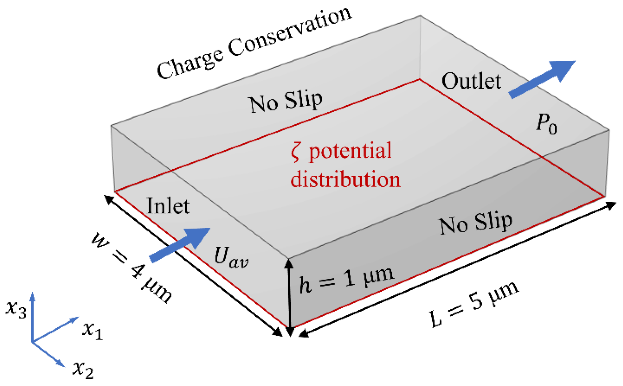
Figure 2.
The non-uniform 2D ζ potential distribution with 1/m, , mV and .

Figure 3.
The meshing of solution domain: (a) the thin-layer region (the schematic is scaled up to 10 times in the direction) and (b) the large bulk region.
Figure 3.
The meshing of solution domain: (a) the thin-layer region (the schematic is scaled up to 10 times in the direction) and (b) the large bulk region.
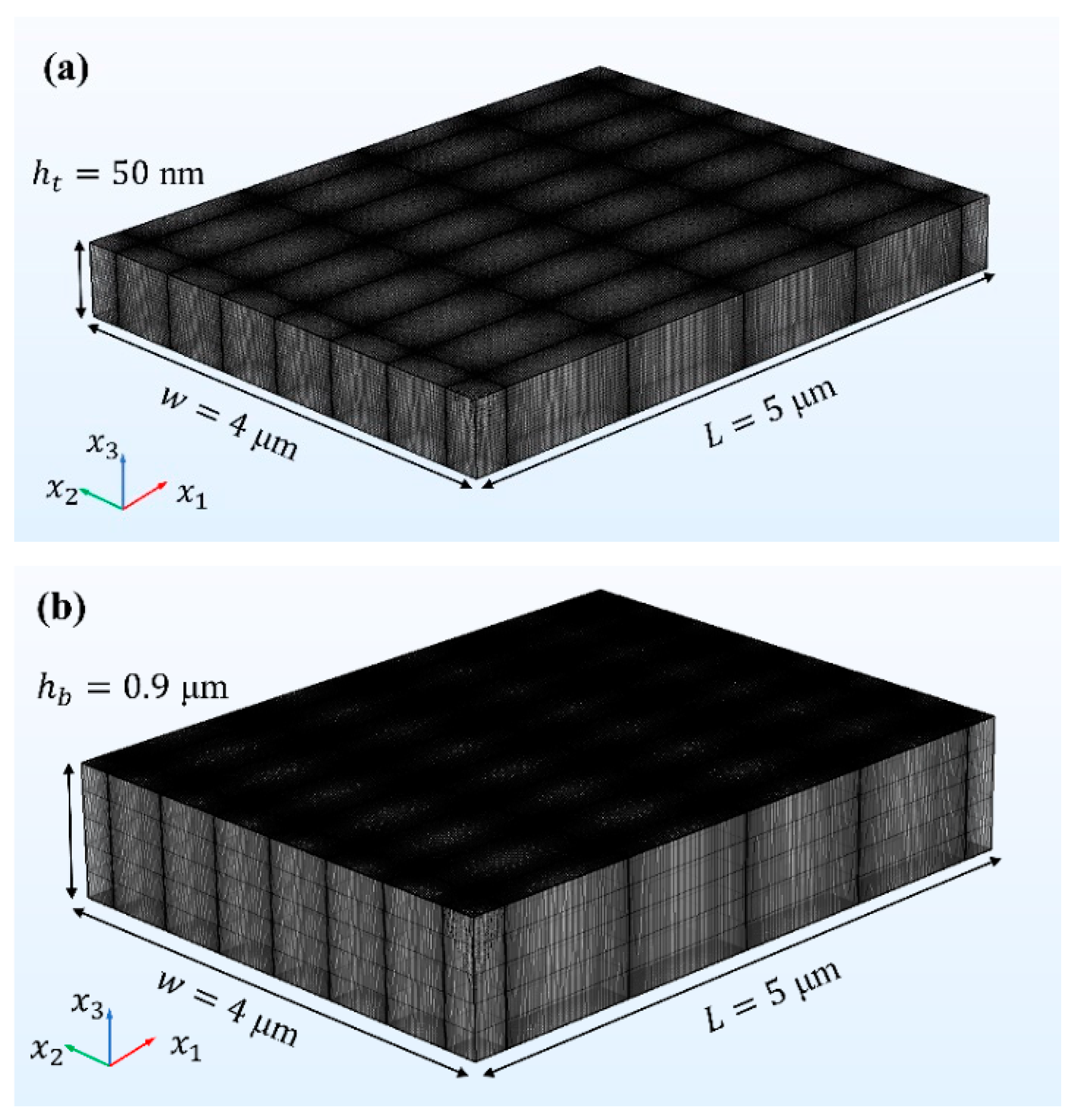
Figure 4.
Grid independence analysis. Plot of relative errors on the computation of velocity, versus the grid quantity , with 1/m, , mV and .
Figure 4.
Grid independence analysis. Plot of relative errors on the computation of velocity, versus the grid quantity , with 1/m, , mV and .

Figure 5.
Velocity distributions. (a) 3D distribution of fluid velocity of basic flow. The magnitudes of , i.e., , is demonstrated by color. The direction of , evaluated by , is demonstrated by the arrows with unit length. (b) Plot of the streamwise velocity component of basic flow, , versus at different with . (c) Plot of streamwise velocity component, , versus at different , where and with 1/m, mV and .

Figure 6.
Potential, electric volume force, and velocity fields generated by uniform ζ potential with mV. 3D distribution of (a) electroosmotic potential (b) electric volume force , and (c) fluid velocity .
Figure 6.
Potential, electric volume force, and velocity fields generated by uniform ζ potential with mV. 3D distribution of (a) electroosmotic potential (b) electric volume force , and (c) fluid velocity .
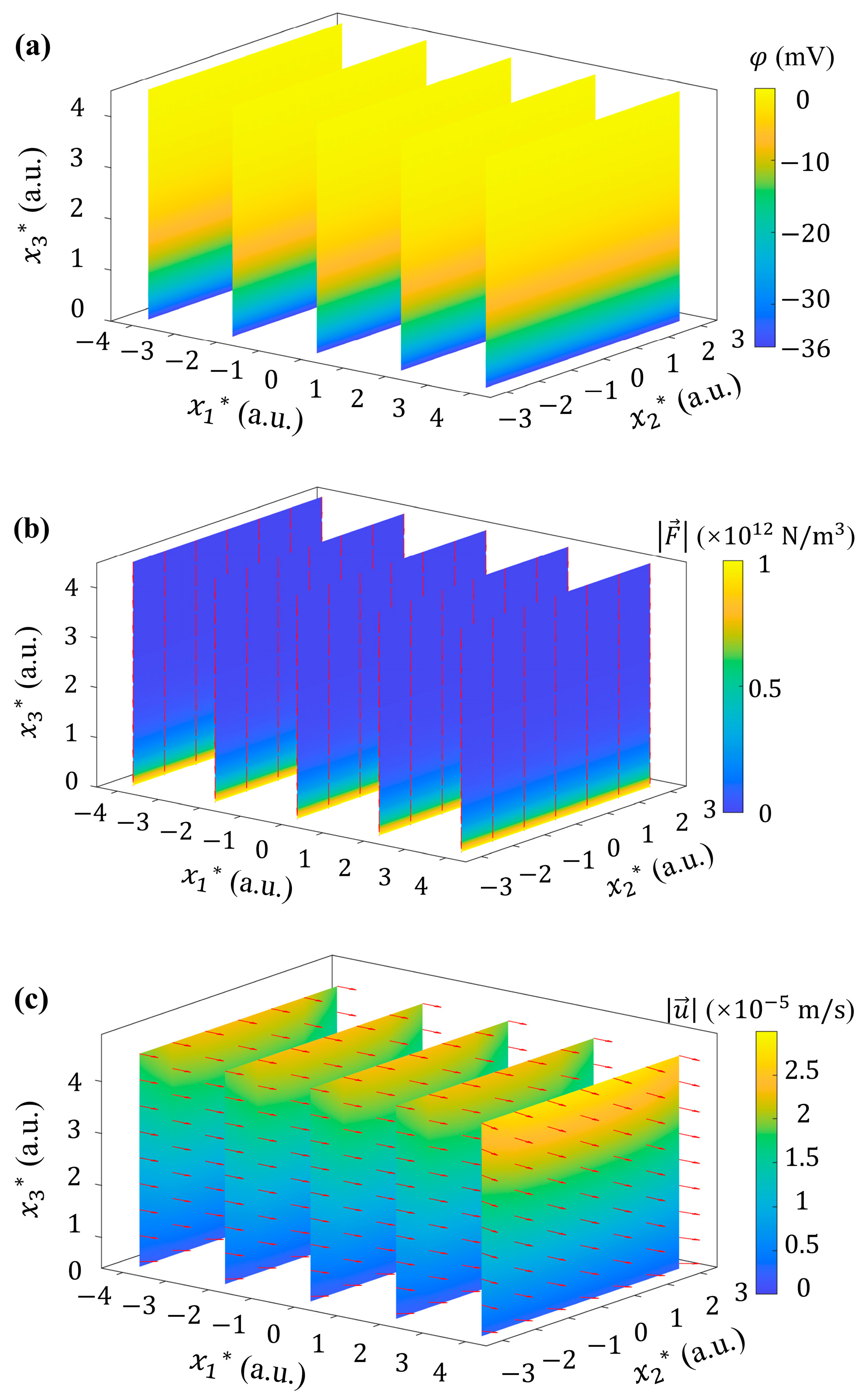
Figure 7.
Electric field and flow field generated by 1D ζ potential with 1/m and mV. (a) 1D distribution of ζ potential. 3D distribution of (b) electroosmotic potential , (c) electric volume force , (d) the curl of electric volume force , and (e) fluid velocity under this 1D ζ potential distribution.


Figure 8.
Potential, and generated by 2D ζ potential with 1/m, , mV and . (a) 3D distribution of . (b) 3D distribution of electric volume force . (c,d) 3D distribution of .
Figure 8.
Potential, and generated by 2D ζ potential with 1/m, , mV and . (a) 3D distribution of . (b) 3D distribution of electric volume force . (c,d) 3D distribution of .

Figure 9.
Velocity and vorticity fields generated by 2D ζ potential with 1/m, , mV and . (a) 3D distribution of fluid velocity . (b) 2D velocity distribution of flow considering and without considering ζ potential distribution at . (c) 3D distribution of the curl of fluid velocity , denoted by , with . Here, is the maximum of basic flow.
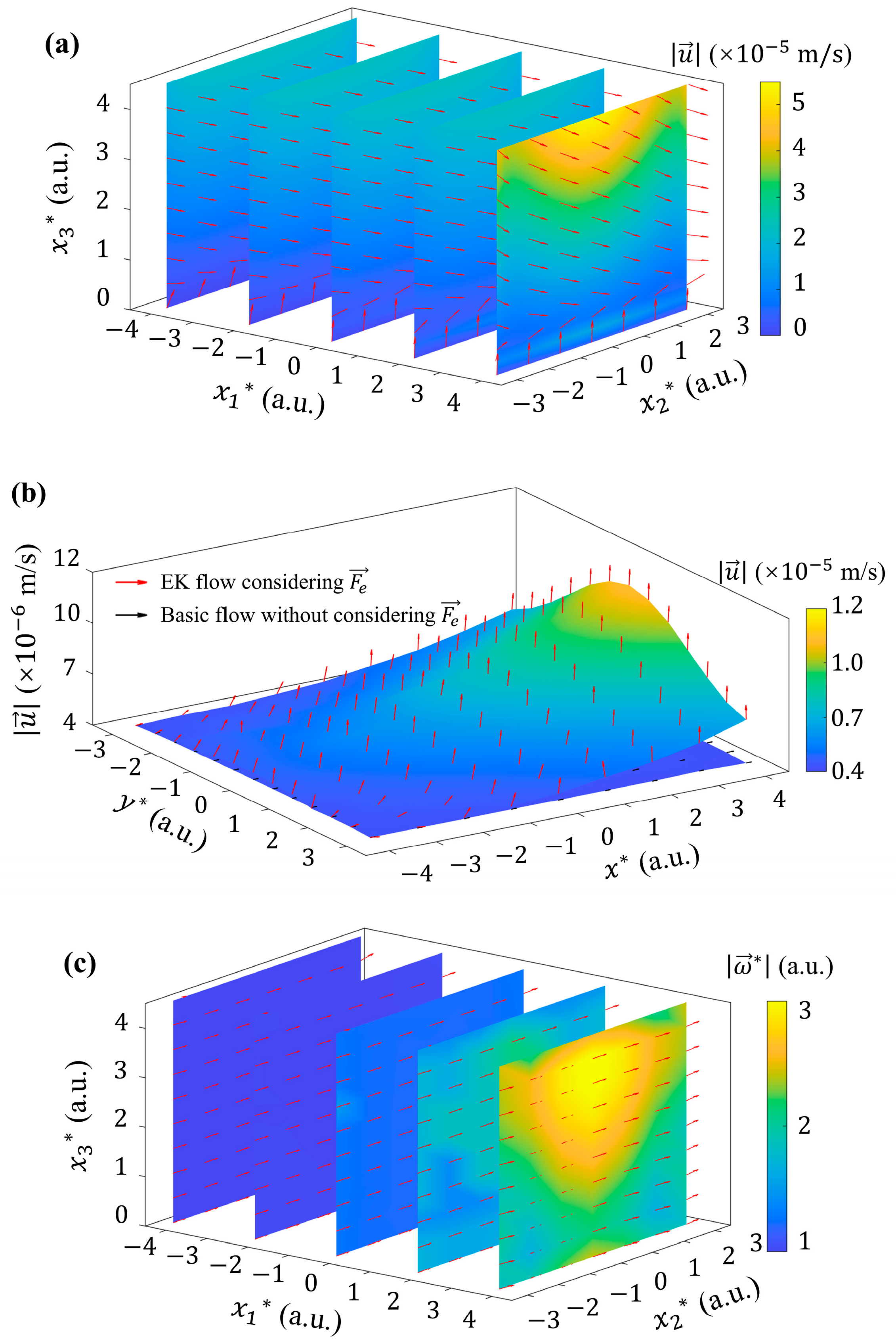
Figure 10.
Influence of on the flow, where and , , mV, and . (a) Plot of streamwise velocity component, , versus dimensional height at different . (b) Plot of streamwise electric volume force component versus slope at the height of . (c) Plot of wall shear stress, , versus dimensional height at different .
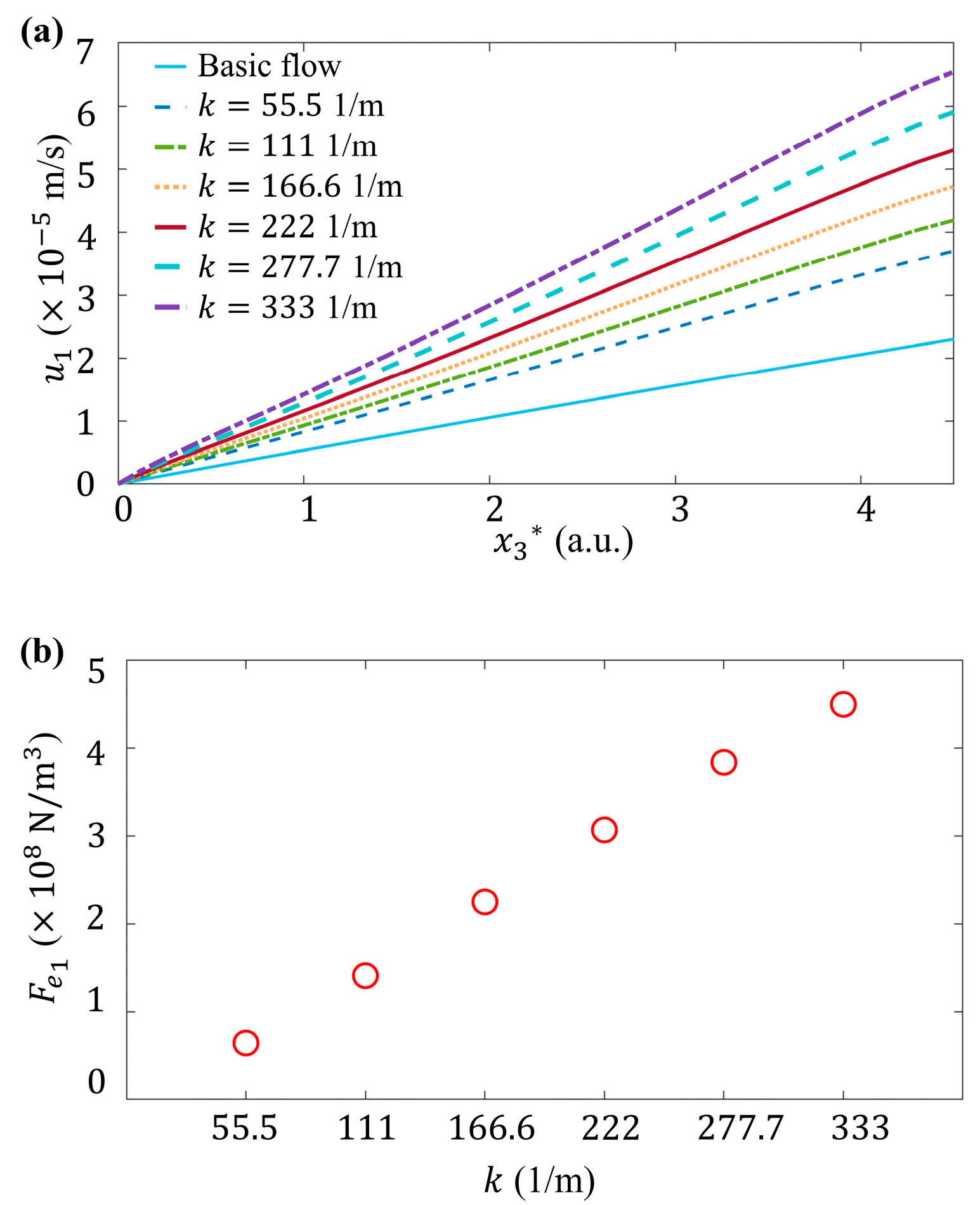
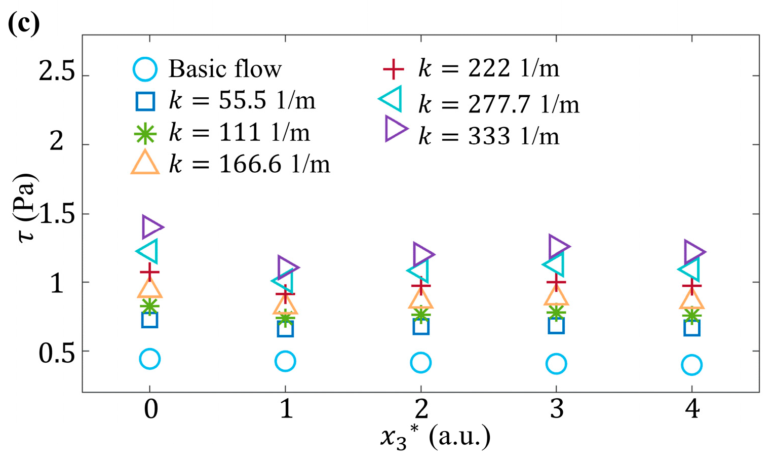
Figure 11.
Influence of on the flow, where and , 1/m, , and . Plot of streamwise velocity component, , versus dimensional height at different .
Figure 11.
Influence of on the flow, where and , 1/m, , and . Plot of streamwise velocity component, , versus dimensional height at different .
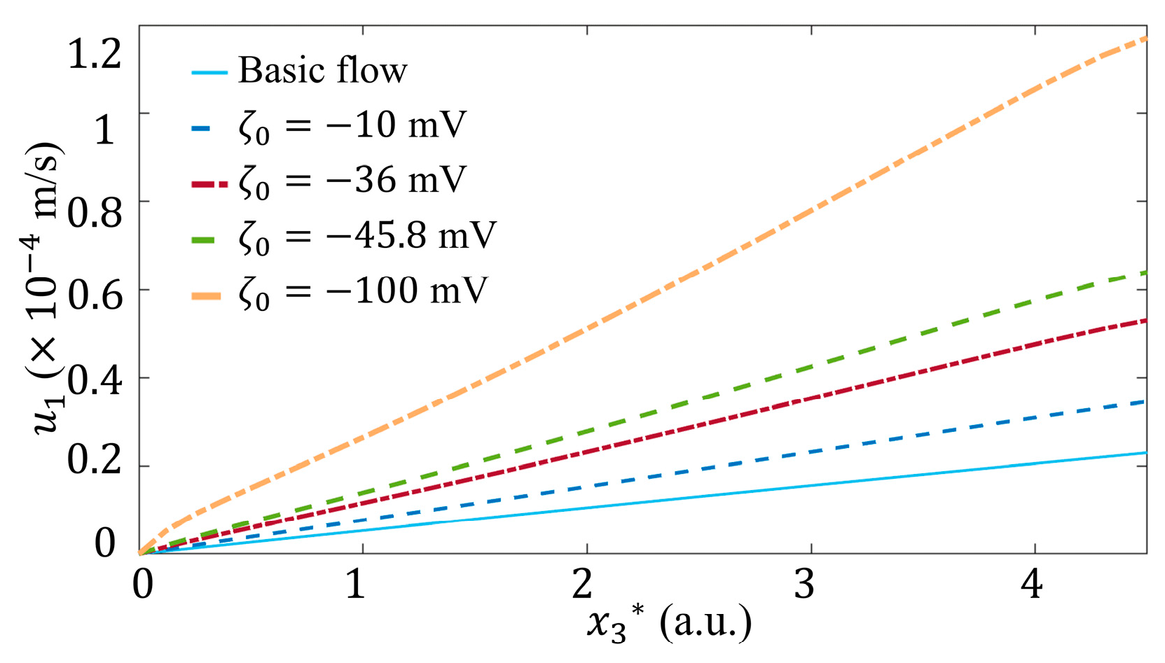
Figure 12.
Influence of on the flow, with 1/m, , and mV. 3D distribution of (a) electric volume force and (b) fluid velocity with wavenumber . (c) Plot of streamwise velocity component, , versus dimensional height at different , where and .
Figure 12.
Influence of on the flow, with 1/m, , and mV. 3D distribution of (a) electric volume force and (b) fluid velocity with wavenumber . (c) Plot of streamwise velocity component, , versus dimensional height at different , where and .


Table 1.
Properties of the material.
| Material | ) | ) | |
|---|---|---|---|
| Liquid water | 997 | 89.57 | 80 |
Table 2.
Detailed information of the grid in the model.
| Parameter | Value |
|---|---|
| Number of grid elements | 7,106,000 |
| Number of grid vertices | 7,275,576 |
| Minimum grid element quality | 1.0 |
| Average grid element quality | 1.0 |
| Grid element volume ratio | |
| Grid volume | μm3 |
| direction | 6.68 nm |
| direction | 20 nm |
| direction | 4.42 nm |
| direction | 13.26 nm |
| direction | 1.33 nm |
| direction | 180 nm |
Disclaimer/Publisher’s Note: The statements, opinions and data contained in all publications are solely those of the individual author(s) and contributor(s) and not of MDPI and/or the editor(s). MDPI and/or the editor(s) disclaim responsibility for any injury to people or property resulting from any ideas, methods, instructions or products referred to in the content. |
© 2024 by the authors. Licensee MDPI, Basel, Switzerland. This article is an open access article distributed under the terms and conditions of the Creative Commons Attribution (CC BY) license (https://creativecommons.org/licenses/by/4.0/).
Share and Cite
MDPI and ACS Style
Han, Y.; Zhao, W. Numerical Simulation of the Influence of Non-Uniform ζ Potential on Interfacial Flow. Micromachines 2024, 15, 419. https://doi.org/10.3390/mi15030419
AMA Style
Han Y, Zhao W. Numerical Simulation of the Influence of Non-Uniform ζ Potential on Interfacial Flow. Micromachines. 2024; 15(3):419. https://doi.org/10.3390/mi15030419
Chicago/Turabian StyleHan, Yu, and Wei Zhao. 2024. "Numerical Simulation of the Influence of Non-Uniform ζ Potential on Interfacial Flow" Micromachines 15, no. 3: 419. https://doi.org/10.3390/mi15030419
Note that from the first issue of 2016, this journal uses article numbers instead of page numbers. See further details here.