Signal Processing Technique for Combining Numerous MEMS Gyroscopes Based on Dynamic Conditional Correlation

Abstract

A signal processing technique is presented to improve the angular rate accuracy of Micro-Electro-Mechanical System (MEMS) gyroscope by combining numerous gyroscopes. Based on the conditional correlation between gyroscopes, a dynamic data fusion model is established. Firstly, the gyroscope error model is built through Generalized Autoregressive Conditional Heteroskedasticity (GARCH) process to improve overall performance. Then the conditional covariance obtained through dynamic conditional correlation (DCC) estimator is used to describe the correlation quantitatively. Finally, the approach is validated by a prototype of the virtual gyroscope, which consists of six-gyroscope array. The experimental results indicate that the weights of gyroscopes change with the value of error. Also, the accuracy of combined rate signal is improved dramatically compared to individual gyroscope. The results indicate that the approach not only improves the accuracy of the MEMS gyroscope, but also discovers the fault gyroscope and eliminates its influence.

1. Introduction

Inertial measurement sensors require smaller size, reliability, low cost and above all accuracy [1]. MEMS technology is widely used in inertial sensors because MEMS gyros have the advantage of low cost, smaller size and easy fabrication in large numbers on a single chip [2,3]. However, these inertial sensors cannot provide highly accurate measurement for the space applications. The accuracy of individual MEMS gyroscope has reached its technology limit. In order to improve the accuracy without breakthrough on hardware, virtual gyroscope technology is presented and accepted by the industry [4]. The method combines multiple gyroscopes to measure the same signal and get the best estimate with data fusion. A “virtual gyroscope” using a four-gyro array was proposed by Bayard and Ploen in [4]. The simulation results showed that the gyroscopes with drifts of 8.66 °/h could be reduced to a virtual gyroscope with a drift of 0.062 °/h when the component gyroscopes are assumed to have a correlation factor of −0.33329. Another two-level optimal filtering method for fusing three gyroscopes was presented by Honglong Chang in [5]. It achieved higher accuracy than individual gyroscope but the continuous-time Kalman filter was not solved to reveal the system property. Stubberud discussed the method of an extend Kalman filter of multiple sensors to improve the accuracy in [6]. Al-Majed and Alsuwaidan presented a multi-filters adaptive estimator to improve the angular rate accuracy by using the noise correlation in [7] but with no simulation or experimental results. Jiang and Xue used six-gyro array in [8,9,10,11]. They also adopted a novel optimal Kalman filter to combine the gyroscopes [8]. Their further study used a first-order Markov process to model the rate signal to improve the performance in dynamic condition [11].

Even the approaches mentioned above have been proven to improve the accuracy effectively, some errors occurring in one or several sensors of the virtual gyroscope may lead to severe accuracy degradation, even wrong results. The key of combining multiple gyroscopes to improve accuracy is the error modeling of individual gyroscope. In above approaches, the random walk, Markov process and Auto Regressive Moving Average (ARMA) were used. All these modeling methods assume that the measured time series has the statistical property at different time. Due to the small size and special structure, MEMS gyro is in fact very sensitive to the change of the surrounding environment. If the power consumption and surrounding temperature change, the statistical features of MEMS gyroscope random drift have big fluctuation. And it exhibits heteroskedasticity. The traditional time series analysis method is not suitable for modeling the random drift error with heteroskedasticity. Unlike the conventional method, Generalized Autoregressive Conditional Heteroskedasticity (GARCH) is able to handle the time series with heteroskedasticity.

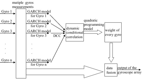
In this paper, based on dynamic conditional correlation (DCC) multivariate GARCH, a dynamic weighted multi-sensors data fusion algorithm is proposed. Firstly, the GARCH process is utilized to model the error of individual MEMS gyroscope. Then the DCC estimator is designed to calculate correlations between multivariate gyroscopes. The DCC estimator has the flexibility of multivariate GARCH but not the complexity. At last, based on the correlation, the optimal weight distribution principle for combining numerous MEMS gyroscope is derived by using quadratic programming. The experimental results show that this approach effectively reduces the noise and eliminates the influence of gyroscope faults.

The paper is organized as follows. The gyroscope error model used in this research is detailed in Section 2. The correlation analysis of gyroscopes based on DCC Multivariate GARCH is derived in Section 3. Mathematical models for combining MEMS Gyroscopes are deduced in Section 4. Numerical experimental results are presented in Section 5. Conclusions are drawn in Section 6.

2. Gyroscope Error Model Based on GARCH

To construct a virtual gyroscope for accuracy improvement, a gyroscope error model is given built firstly. The gyroscope error has heteroskedasticity when surroundings change with time, for instance, temperature. The GARCH process introduced by Bollerslev (1986) [12] is the extension of the Autoregressive Conditional Heteroskedasticity (ARCH) process. This type of model has been proven useful in modeling the time series with heteroskedasticity [13,14,15].

Assume that ε_t is a real-valued discrete-time stochastic process and Ψ_t is the information set of all information through time t. Following [12], the GARCH (p, q) process is then given as:

$$\{\begin{array}{l}{\text{ε}}_t|{\text{ψ}}_t~N(0,h_t)\\ h_t={\text{α}}_0+{\displaystyle \sum _{i=1}^q{\text{α}}_i{\text{ε}}_{t-i}^2}+{\displaystyle \sum _{i=1}^p{\text{β}}_i{h}_{t-i}}\end{array}$$

(1)

where

$$\begin{array}{l}p\ge 0,q\ge 0\\ {\text{α}}_0>0,{\text{ α}}_i>0,i=1,2,\cdots ,q\\ {\text{β}}_i\ge 0,i=1,2,\cdots ,p\\ {\displaystyle \sum _{i=1}^{\max (p,q)}({\text{α}}_i+{\text{β}}_i)}<1\end{array}$$

α_i has to be assumed greater than 0, otherwise the GARCH (p, q) model may not be identified. ${\displaystyle \sum _{i=1}^{\max (p,q)}({\text{α}}_i+{\text{β}}_i)}<1$ defines a sufficient (but not necessary unless p = q = 1) condition for weak stationarity.

In GARCH process, the conditional variance h_t is a linear function of past sample variances, and allows lagged conditional variances to enter as well, The conditional variance changes with time, that is, with heteroskedasticity. Its conditionality shows that this process depends on adjacent empirical information. For the MEMS gyroscopes, “conditional” of h_t means that the random drift is related to its adjacent observations, and reflects autocorrelation of variance of MEMS gyroscope. Auto regression represents the feedback mechanism that the predicted values are associated with the past time. So the GARCH model is suitable for modeling MEMS gyroscope error with heteroskedasticity. In this model, the conditional variance can be estimated with maximum likelihood method.

3. Correlation Analysis of Gyroscopes Based on DCC Multivariate GARCH

In order to determine the weights of each sensor for output data fusion, correlations between MEMS gyroscope should be analyzed. In fact, correlations between gyros are not constant. Especially, when there is large deviation in some gyroscope output, the correlations between the gyroscopes will also dramatically change accordingly. Reliable estimates of correlation and its variation are significant for reducing error influenced by gyroscope faults.

3.1. DCC Model

Multivariate GARCH model can examine the dynamic relationship between multiple time series. While univariate GARCH models have achieved widespread empirical success, the question on estimations of multivariate GARCH models with time-varying correlations has been the motivation for countless academic articles and practitioner conferences. The methods, such as the BEKK (named after Baba, Engle, Kraft and Kroner) and constant conditional correlation (CCC) model, are widely used [16,17]. In most cases, if the number of estimated parameters is large, the computation load could be too huge to carry on, especially when there are more than five data sequences considered. The DCC multivariate GARCH model is proposed by Engle (2002) [18]. Compared to other models, DCC ensures positive definiteness but does not produce valid correlation generally. It preserves the parsimony of univariate GARCH models, and greatly decreases the number of estimated parameters, as well as the number of simultaneously estimated parameters. The virtual gyroscope in this paper is composed of six gyroscopes, which means that six data sequences will be considered and DCC models have to be used to estimate the large conditional covariance matrix which can be used to describe the correlation between gyroscopes. In addition, for the extended models of DCC, the conditioning set in them may be too large.

Assuming that the residuals of output rate signal of n gyroscopes are conditionally multivariate normal with zero expected value and covariance matrix H_t, the multivariate GARCH model is given by [18]:

$$r_t|{\Omega }_{t-1}~N(0,H_t)$$

(2)

and

$$H_t=D_t{R}_t{D}_t,\text{ where }{D}_t=diag\left\{\sqrt{h_{i,t}}\right\}$$

(3)

where r_t refers to output rate signal of gyroscopes, Ω_t−1 is the information set through time t − 1 and R_t is the time varying correlation. The expression for h is proposed to write as univariate GARCH model as Equation (1). The proposed dynamic correlation structure is given as follows [18]:

$$Q_t=(1-{\displaystyle \sum _{m=1}^M{a}_m}-{\displaystyle \sum _{n=1}^N{b}_n})S+{\displaystyle \sum _{m=1}^M{a}_m}{\text{ε}}_{t-m}{\text{ε}}_{t-m}^{\prime }+{\displaystyle \sum _{n=1}^N{b}_n}{Q}_{t-n}$$

(4)

$$R_t=diag(q_{11,t}^{-\frac{1}{2}},\cdots ,q_{nn,t}^{-\frac{1}{2}})\circ Q_t\circ diag(q_{11,t}^{-\frac{1}{2}},\cdots ,q_{nn,t}^{-\frac{1}{2}})$$

(5)

where, ${\text{ε}}_t=D_t^{-1}{r}_t$ and S is the unconditional correlation matrix of the epsilons. And

$$a_m>0,b_n\ge 0,{\displaystyle \sum _{m=1}^M{a}_m}+{\displaystyle \sum _{n=1}^N{b}_n}<1$$

where m and n are lag intervals.

In Equation (5), “°” is the Hadamard product of two identically sized matrices. q_ij,t is the element of Q_t, so that the typical element of R_t is deduced as:

$${\text{ρ}}_{ij,t}=\frac{q_{ij,t}}{\sqrt{q_{ii,t}{q}_{jj,t}}}$$

(6)

3.2. Estimating Parameters

The model parameters can be estimated through maximum likelihood (ML). The log likelihood of this estimator can be expressed as:

$$\begin{array}{l}L=-\frac{1}{2}{\displaystyle \sum _{t=1}^T(n\log (2\text{π})+\log (\left|H_t\right|)+r_t^{\prime }{H}_t^{-1}{r}_t)}\\ =-\frac{1}{2}{\displaystyle \sum _{t=1}^T(n\log (2\text{π})+\log (\left|D_t{R}_t{D}_t\right|)+r_t^{\prime }{D}_t^{-1}{R}_t^{-1}{D}_t^{-1}{r}_t)}\\ =-\frac{1}{2}{\displaystyle \sum _{t=1}^T(n\log (2\text{π})+2\log (\left|D_t\right|)+r_t^{\prime }{D}_t^{-1}{D}_t^{-1}{r}_t}\\ -{\text{ε}}_t^{\prime }{\text{ε}}_t+\log (\left|R_t\right|)+{\text{ε}}_t^{\prime }{R}_t^{-1}{\text{ε}}_t)\end{array}$$

(7)

Let θ stand for the parameters in D_t and ϕ stand for the additional parameters in R_t. The log likelihood is rewritten as follows:

$$L(\text{θ},\varphi )=L_V(\text{θ})+L_C(\text{θ},\varphi )$$

(8)

where, L_v(θ) is the volatility and L_c(θ, ϕ) is the correlation.

The volatility term is shown as:

$$L_V(\text{θ})=-\frac{1}{2}{\displaystyle \sum _t(n\log (2\text{π})+2\log (\left|D_t\right|)+r_t^{\prime }{D}_t^{-1}{D}_t^{-1}{r}_t)}$$

(9)

and the correlation component is expressed as:

$$L_C(\text{θ},\varphi )=-\frac{1}{2}{\displaystyle \sum _t(\log (\left|R_t\right|)+{\text{ε}}_t^{\prime }{R}_t^{-1}{\text{ε}}_t-{\text{ε}}_t^{\prime }{\text{ε}}_t)}$$

(10)

The DCC model is designed and used in two stage estimation. In the first stage, unvariate GARCH models are estimated and the volatility part is the sum of individual GARCH likelihoods:

$$L_V(\text{θ})=-\frac{1}{2}{\displaystyle \sum _t{\displaystyle \sum _{i=1}^n(\log (2\text{π})+\log (h_{i,t})+\frac{r_{i,t}^2}{h_{i,t}})}}$$

(11)

In the second stage, the correlation parameters can be estimated by using correlation part likelihood, conditioning on the parameters estimated in first stage.

The two-step approach to maximizing can be expressed as follows:

$$\widehat{\text{θ}}=\arg \max \left\{L_V(\text{θ})\right\}$$

(12)

$$\underset{\varphi }{\max }\left\{L_C(\widehat{\text{θ}},\varphi )\right\}$$

(13)

Then the conditional covariance matrix H_t is obtained and the correlations between outputs of gyroscopes are estimated. Since the number of parameters estimated in the correlation process is independent of the number of series correlated, large correlation matrices can be estimated.

3.3. Hypothesis Testing

After estimating the parameters in model, the hypothesis test needs to be done for R_t in order to judge the presence of dynamic time-varying relationship between multiple gyroscopes. The method is described as follows:

$$H_{\text{0}}:R_t=\overline{R}{H}_{\text{1}}:R_t\ne \overline{R}$$

(14)

Then the test is carried out through the distribution approach proposed by Engle [19], meanwhile the P-value is obtained.

4. Mathematical Models for Combining MEMS Gyroscopes

To make full use of the time-varying correlation information of MEMS gyroscopes for accuracy improvement, dynamic weighted multi-sensors data fusion method is proposed in this paper.

Assume that w_t = (w_1t, …, w_nt) are the weights of gyroscopes, where ${\displaystyle \sum _{i=1}^n{w}_{it}}=1$, t = 1, 2, …, T, n is the number of gyroscopes, and T is sampling number. Then the conditional covariance after data fusion is:

$$\begin{array}{l}{h}_{f,t}={\displaystyle \sum _{i=1}^n{\displaystyle \sum _{j=1}^n{w}_{it}{w}_{jt}\sqrt{h_{i,t}}\sqrt{h_{j,t}}{\text{ρ}}_{ij,t}}}\\ ={\displaystyle \sum _{i=1}^n{\displaystyle \sum _{j=1}^n{w}_{it}{w}_{jt}{h}_{ij,t}}}\\ =w_t^T{H}_t{w}_t\end{array}$$

(15)

where ρ_ij,t is correlation coefficient in Equation (6), and H_t is conditional covariance which is defined in Section 3. Then the quadratic programming model for dynamic weighted fusion can be given by:

$$\begin{array}{l}Min:w_t^T{H}_t{w}_t\\ S.T\{\begin{array}{l}{\displaystyle \sum _{i=1}^n{w}_{it}}=1,0\le w_{it}\le 1\\ H_t=D_t{R}_t{D}_t(\text{DCC})\end{array}\end{array}$$

(16)

This model is used to obtain the weight of each gyroscope, which can minimize the conditional variance of the outputs from virtual gyroscope. The first constraint condition means that the sum of weights must be 1 and the weights should between 0 and 1. The second constraint means that the conditional variance matrix H_t is computed by DCC multivariate GARCH models.

The weights w_t can be obtained by solving this model with active set method. Then the output of the gyroscope array can be expressed as:

$${\widehat{Y}}_t=Y_t{w}_t^{\prime },t=1,2,\cdots ,T$$

(17)

where Y_t = (y_1t, y_{2t, …,} y_nt) and y_nt is output rate signal of individual MEMS gyroscope. To update the gyroscope weights in real time, a rolling window is used in re-estimating the model, which means that the models are estimated first from the data in time T, and then the weights are calculated. After obtaining new observations in a period of time t₀, the models are re-estimated and new weights calculated for time T + t₀.

5. Experiments and Results

Six separate ADXRS300 [20] gyroscopes were taken to construct a gyroscope array. A prototype of the virtual gyroscope is shown in Figure 1.

The bandwidth of individual gyroscope is set to 40 Hz by choosing proper application circuit. To satisfy the Nyquist theorem, the sampling rate is set to 200 Hz. The original output signal of the ADXRS300 is a voltage proportional to angular rate. To obtain the output angular rate signal, we acquire the relationship between the output voltage of gyroscopes and input angular rates through the calibration, which is shown in Figure 2. Then the output voltage is converted to the rate signal.

Figure 1. Prototype of the virtual gyroscope.

Figure 1. Prototype of the virtual gyroscope.

Figure 2. Scale factor plot of the individual gyroscopes.

Figure 2. Scale factor plot of the individual gyroscopes.

3600 observations are collected when the input angular rate maintains zero. Output rate signals of the individual gyroscopes are shown in Figure 3. The experiments are performed at the room temperature (around 25 °C), meanwhile the gyros internal temperature, which is shown in Figure 4, changes with time because of self-heating.

Figure 3. Outputs of the individual gyroscopes.

Figure 3. Outputs of the individual gyroscopes.

Figure 4. Internal temperature of gyros

Figure 4. Internal temperature of gyros

From Figure 3, it can be seen that the error of Gyro 4 is for larger than usual, especially from 1000 s to 3600 s, while outputs of other gyroscopes appear normally. The environmental conditions of each gyro in the array are identical, so the output of Gyro 4 is not normal and the abnormality of Gyro 4 is due to internal fault. If Kalman filter or other conditional approaches to combining the gyroscopes are used, the accuracy will be decreased.

Autoregressive Conditional Heteroskedasticity (ARCH) effect is the precondition to apply GARCH model to the measured time series, so that ARCH effect test is necessary before gyroscopes are modeled. The commonly used method Lagrange multiplier (LM) proposed by Engle (1982) [19] is applied to test the ARCH effect of outputs of gyroscopes. The test results under the condition of 1 lag interval are shown in Table 1.

Table 1. Test results of Autoregressive Conditional Heteroskedasticity (ARCH) effect.

Gyros	P-Value	LM-Statistic
Gyro 1	0.0000	138.0458
Gyro 2	0.0000	284.1072
Gyro 3	0.0000	835.0323
Gyro 4	0.0000	1621.1489
Gyro 5	0.0000	305.1508
Gyro 6	0.0000	293.7068

Table 1. Test results of Autoregressive Conditional Heteroskedasticity (ARCH) effect.

Gyros	P-Value	LM-Statistic
Gyro 1	0.0000	138.0458
Gyro 2	0.0000	284.1072
Gyro 3	0.0000	835.0323
Gyro 4	0.0000	1621.1489
Gyro 5	0.0000	305.1508
Gyro 6	0.0000	293.7068

Table 1 shows that the LM statistics of each gyroscope are larger than critical value, and the value of P is almost zero. Therefore, we reject the null hypothesis and ARCH effect is of certification in the measured time series of each single gyroscope, which means that the GARCH model can correctly describe the measured time series.

Therefore, we use GARCH model to combine the gyroscopes. Firstly, we determine the order of GARCH model. To reduce the complexity of model, p and q should be as small as possible. And in general case, GARCH (1, 1) model can feature the data well, so we choose GARCH (1, 1) to model individual gyroscopes. For the rolling window, the size of the window is set to be 360, and the movement speed of the window is set to be 30.

Obtaining conditional covariance matrix H_t is performed in two steps. Now first 360 observations are taken as example to estimate the parameters of GARCH.

Step 1: GARCH (1, 1) is used to model each gyroscope, which means that the parameters in Equation (11) are estimated under the condition of p = q = 1.The mean equation and variance equation can be given by: $y_t=y_{t-1}+{\text{ε}}_t;h_t^2={\text{α}}_0+{\text{αε}}_{t-1}^2+\text{β}{h}_{t-1}^2$, where y_t is the residuals of output rate signal of individual MEMS gyroscope. The estimated results of GARCH (1, 1) for individual gyroscope are shown in Table 2. In this table, α₀ is the constant term in GARCH model according to Equation (1), α is the coefficient of past sample variances of MEMS gyroscopes, and β is the coefficient of lagged conditional variances of MEMS gyroscopes. In general, the outputs of each gyroscope accord with the assumptions of GARCH (1, 1).

Step 2: After Estimating the parameters in Equation (10) through ML method in Equation (13), a = 0.0310, b = 0.9484 are obtained, whose standard deviation are 1.57 × 10⁻⁵ and 0.0084. The results show that all dynamic correlation coefficient are greater than zero, which means that the correlation coefficient matrix and prophase influence have positive correlation. Moreover, the closer the value of b to 1, the greater correlation coefficient influenced by prophase part.

Table 2. Estimated results of Generalized Autoregressive Conditional Heteroskedasticity (GARCH) (1, 1).

Gyros	α0		α		β
	Value	Standard Deviation	Value	Standard Deviation	Value	Standard Deviation
Gyro 1	4.94 × 10−4	7.08 × 10−9	0.031432	1.57 × 10−5	0.685944	0.001411
Gyro 2	1.07 × 10−4	4.32 × 10−9	0.039131	0.000914	0.904651	0.000235
Gyro 3	1.43 × 10−4	8.16 × 10−9	0.086132	0.000565	0.865696	6.87 × 10−5
Gyro 4	8.60 × 10−5	1.62 × 10−9	0.081163	3.24 × 10−5	0.916089	0.001028
Gyro 5	1.28 × 10−4	1.89 × 10−9	0.039739	0.004628	0.906221	5.47 × 10−5
Gyro 6	5.19 × 10−4	3.25 × 10−9	0.057514	0.001625	0.681433	0.000963

Table 2. Estimated results of Generalized Autoregressive Conditional Heteroskedasticity (GARCH) (1, 1).

Gyros	α0		α		β
	Value	Standard Deviation	Value	Standard Deviation	Value	Standard Deviation
Gyro 1	4.94 × 10−4	7.08 × 10−9	0.031432	1.57 × 10−5	0.685944	0.001411
Gyro 2	1.07 × 10−4	4.32 × 10−9	0.039131	0.000914	0.904651	0.000235
Gyro 3	1.43 × 10−4	8.16 × 10−9	0.086132	0.000565	0.865696	6.87 × 10−5
Gyro 4	8.60 × 10−5	1.62 × 10−9	0.081163	3.24 × 10−5	0.916089	0.001028
Gyro 5	1.28 × 10−4	1.89 × 10−9	0.039739	0.004628	0.906221	5.47 × 10−5
Gyro 6	5.19 × 10−4	3.25 × 10−9	0.057514	0.001625	0.681433	0.000963

Meanwhile, according to the hypothesis test in Equation (14), P-value is 0 and chi-square value is 180.24. The chi-square test shows obvious statistical significance. So the null hypothesis H₀ in Equation (14) is rejected and H₁ is admitted, which means that there is dynamic time-varying relationship between multiple gyroscopes.

Then move the window and re-estimate the models. In every window, once all parameters in DCC have been estimated, H_t and correlation coefficient matrix R_t is also estimated, which is shown in Figure 5 and Figure 6, respectively. Due to h_ij,t = h_ji,t, ρ_ij,t = ρ_ji,t, ρ_ii,t = 1 (i, j = 1, 2, …, 6), only the curves of h_ij,t (i < j) and ρ_ij,t (i < j) are given in the figures.

Then take H_t in Equation (16) and solve the quadratic programming. The obtained weights are depicted in Figure 7.

Figure 5. H_t estimated.

Figure 5. H_t estimated.

Figure 6. Curve of dynamic correlation coefficient.

Figure 6. Curve of dynamic correlation coefficient.

Figure 7. Weights of the individual gyroscopes.

Figure 7. Weights of the individual gyroscopes.

From Figure 7, it can be seen that the weight of each gyroscope is time-varying, and the variation corresponds to conditional correlation coefficient. It is worth noting that the weight of Gyro 4 has a declining trend, as expected, especially near zero after 2500 s, which is relevant to the large error of Gyro 4. Because the error of Gyro 4 is larger than other gyros, the accuracy may be decreased when combining the gyroscopes to a virtual gyroscope with other approaches. However, with the method in this article, according to Equation (17), when the weight of the Gyro 4 is smaller, the influence of Gyro 4 on accuracy of virtual gyroscope is weaker. In addition, the weights are obtained through the model in Section 4, and this model is used to obtain the weight of each gyroscope, which can minimize the conditional variance of the outputs from virtual gyroscope. So the accuracy can be improved more compared to the six gyroscopes when the weight of the Gyro 4 is smaller. It proves that the data fusion scheme can eliminate the influence of malfunction gyroscope in gyroscope array. Then the outputs of MEMS gyroscope can be combined by Equation (17). 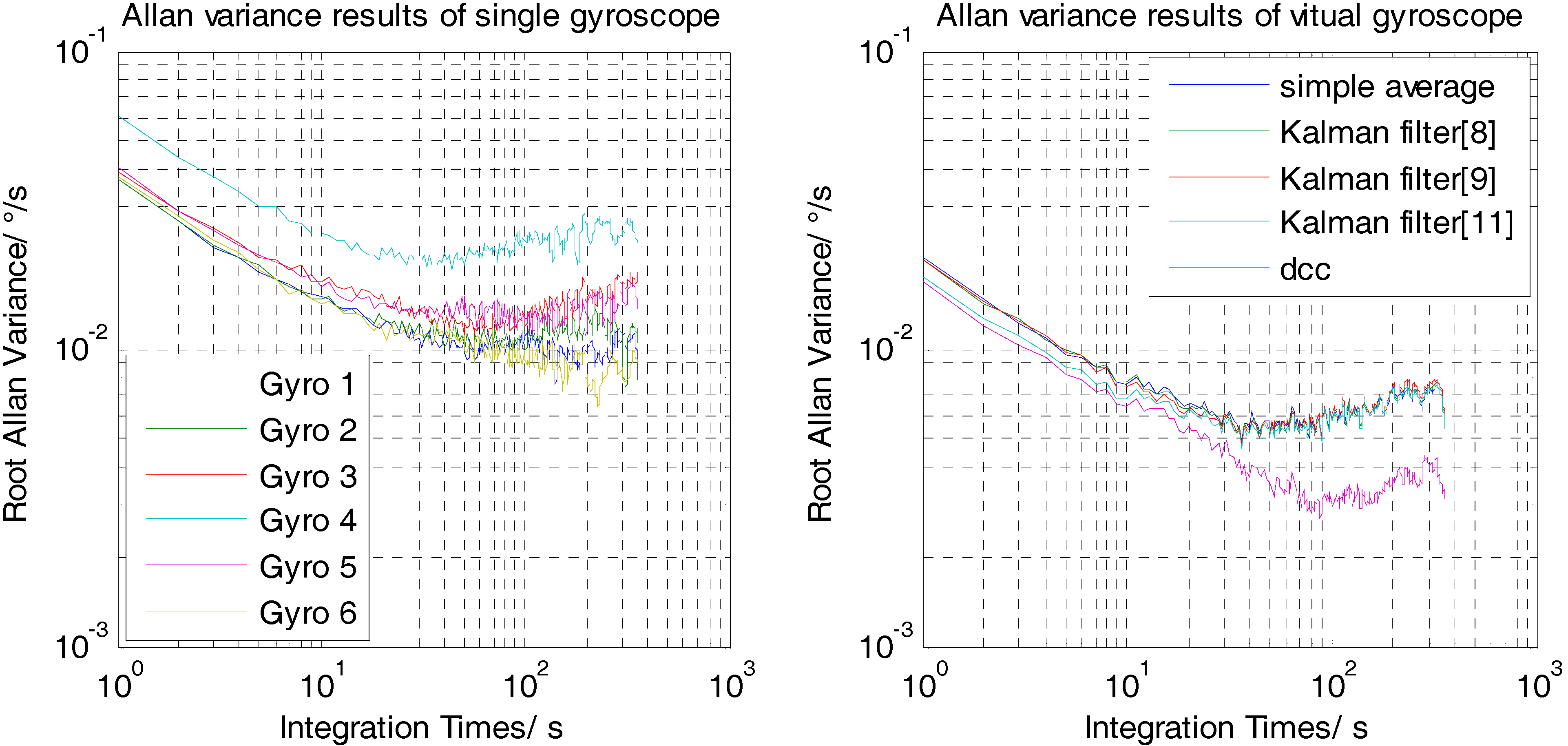Finally, the outputs of virtual gyroscope are shown in Figure 8. The comparisons of Allan variance measurements between the virtual gyro and single gyro are shown in Figure 9. And the detailed results are illustrated in Table 3. The simple average and the Kalman filter in [8,9,11] are competitors. In this paper, the accuracy means the closeness between the results of measurement and the true angular rate, which can be represented by the amount of measurements errors. Then the standard deviation (1σ), the mean of the estimated errors, the angular random walk (ARW) noise and bias drift are used to evaluate the accuracy of the rate signal, thus the improvement factor is define as:

$$I{F}_i=i_{Sgyro}/i_{Vgyro}$$

(18)

where IF_i is the improvement factor and I refers to 1σ errors, mean, ARW noise and bias drift. i_Sgyro is 1σ errors, mean, ARW noise or bias drift for the single gyroscope in the array, and i_Vgyro is that for the virtual gyroscope. Alternatively, we use the average of the six gyroscopes to represent the single gyroscope here when calculate IF_i because the accuracy of the gyroscopes is different.

Table 3 shows that the 1σ estimated errors of gyroscopes are reduced from 0.0418–0.0545 °/s (except Gyro 4) to 0.0189–0.0231 °/s by five different models. Therefore, the performance improvement by these five different models is nearly equivalent, and the DCC multivariate GARCH has a slight edge.

However, in the view of mean, we know it increases from 0.0066–0.0110 °/s (except Gyro 4) to 0.0239–0.0243 °/s by simple average and Kalman filters, which indicates that these four models are out of work for performance improvement under the influence of Gyro 4. Compared with other models, the mean of virtual gyroscope combined by DCC model is reduced to 0.0047 °/s, so that the performance is also improved, and the improvement factor of the accuracy is about 5.17.

Figure 8. Outputs of virtual gyroscope.

Figure 8. Outputs of virtual gyroscope.

Figure 9. Allan variance results of the virtual gyro compared to the single gyro.

Figure 9. Allan variance results of the virtual gyro compared to the single gyro.

Table 3. Experiments results.

Model	Mean (°/s)	1σ (°/s)	ARW ($°/\sqrt{\text{h}}$)	Bias Drift (°/h)
Gyro 1	0.0086	0.0418	1.74	38.02
Gyro 2	0.0092	0.0436	1.74	38.88
Gyro 3	0.0110	0.0545	1.86	42.52
Gyro 4	0.1022	0.1051	2.94	73.19
Gyro 5	0.0082	0.0484	1.85	47.02
Gyro 6	0.0066	0.0446	1.73	32.78
Simple average	0.0243	0.0231	1.03	19.91
Kalman filter [8]	0.0240	0.0227	1.02	19.18
Kalman filter [9]	0.0239	0.0227	1.01	19.18
Kalman filter [11]	0.0239	0.0225	0.96	18.96
DCC	0.0047	0.0189	0.93	11.02
IF of DCC	5.17	2.98	2.13	4.09

Table 3. Experiments results.

Model	Mean (°/s)	1σ (°/s)	ARW ($°/\sqrt{\text{h}}$)	Bias Drift (°/h)
Gyro 1	0.0086	0.0418	1.74	38.02
Gyro 2	0.0092	0.0436	1.74	38.88
Gyro 3	0.0110	0.0545	1.86	42.52
Gyro 4	0.1022	0.1051	2.94	73.19
Gyro 5	0.0082	0.0484	1.85	47.02
Gyro 6	0.0066	0.0446	1.73	32.78
Simple average	0.0243	0.0231	1.03	19.91
Kalman filter [8]	0.0240	0.0227	1.02	19.18
Kalman filter [9]	0.0239	0.0227	1.01	19.18
Kalman filter [11]	0.0239	0.0225	0.96	18.96
DCC	0.0047	0.0189	0.93	11.02
IF of DCC	5.17	2.98	2.13	4.09

From the Allan variance plot, both the ARW noise and bias drift are reduced by fusing multiple measurements from gyro array. Table 3 reveals that the ARW noise of the gyroscope is reduced from 1.73–2.94 $°/\sqrt{\text{h}}$ to 0.96–1.93 $°/\sqrt{\text{h}}$ by simple average and Kalman filters. Meanwhile, the bias drift is reduced from 32.78–73.19 °/h to 18.96–19.91 °/h. The ARW noise and bias drift are reduced to 0.93 $°/\sqrt{\text{h}}$ and 11.02 °/h by the DCC model, indicating a bias drift reduction factor of about 4.09, which is larger than the other models.

From the experimental results above, we find out that fusing multiple measurements from gyroscope array for accuracy improvement has higher reliability and effectiveness based on DCC model.

6. Conclusions

In this paper, based on DCC multivariate GARCH, a dynamic weighted multi-sensors data fusion algorithm is proposed to improve the overall accuracy of the MEMS gyroscopes. The GARCH model has been established to model the rate signal for MEMS gyroscope, and the dynamic conditional correlation between gyroscopes, which is significant for combining numerous gyroscopes, is analyzed by DCC multivariate GARCH. It indicates that the six-gyroscope array with an ARW noise of 1.73–2.94 $°/\sqrt{\text{h}}$ and a bias drift of 32.78–73.19 °/h are combined into a rate signal having an ARW noise of 0.93 $°/\sqrt{\text{h}}$ and a bias drift of 11.02 °/h, even the error of one gyroscope in the array is larger than usual. Compare to other fusion approaches, the proposed method can not only improve the accuracy more greatly, but also eliminate the influence of faulty gyros. It proved that the dynamic weighted multi-sensors data fusion algorithm based on DCC multivariate GARCH is efficient and reliable for modeling rate signal to improve the system overall performance.

In the future fabrication of a number of MEMS gyroscopes on a single chip would enhance the uniformity between the gyroscopes and the correlation between the gyroscopes in the same array would be more significant. Through the proposed method, the MEMS industry can produce gyroscopes with higher accuracy and higher reliability at a low cost.