An Integrated Statistical and Clinically Applicable Machine Learning Framework for the Detection of Autism Spectrum Disorder

Abstract

Autism Spectrum Disorder (ASD) is a neurological impairment condition that severely impairs cognitive, linguistic, object recognition, interpersonal, and communication skills. Its main cause is genetic, and early treatment and identification can reduce the patient’s expensive medical costs and lengthy examinations. We developed a machine learning (ML) architecture that is capable of effectively analysing autistic children’s datasets and accurately classifying and identifying ASD traits. We considered the ASD screening dataset of toddlers in this study. We utilised the SMOTE method to balance the dataset, followed by feature transformation and selection methods. Then, we utilised several classification techniques in conjunction with a hyperparameter optimisation approach. The AdaBoost method yielded the best results among the classifiers. We employed ML and statistical approaches to identify the most crucial characteristics for the rapid recognition of ASD patients. We believe our proposed framework could be useful for early diagnosis and helpful for clinicians.

1. Introduction

Autism Spectrum Disorder (ASD) is a group of neurological diseases that hinder the normal progression of the brain [1]. ASD causes social difficulties, sensory issues, repetitive behaviour, and intellectual incapacity. ASD patients also have psychiatric or neurological disorders such as hyperactivity, attention deficit, anxiety, sadness, and epilepsy [2].

ASD has been connected to genetics and physiological factors. However, the disorder is often assessed utilizing non-genetic behavioural criteria. Autism symptoms are more apparent and easier to recognize in youngsters between 2 and 3 years old. ASD affects one in 68 children in the United States, according to [2]. Existing statistics indicate that approximately 1.5% of the global population is autistic, and it is assumed that a large proportion of autistic people remain unidentified. Consequently, there is a strong need for rapid diagnosis facilities due to the increased recognition of ASD.

Traditional diagnostic approaches for ASD involve medical practitioners undertaking a clinical evaluation of the patient’s psychological age during clinical assessment. This generally acknowledged method is called Clinical Judgment (CJ). Autism Diagnostic Interview (ADI) and The Autism Diagnostic Observation Schedule (ADOS) are another two conventional diagnostic techniques [3]. A formal diagnosis of autism spectrum disorder is a lengthy procedure since it involves time for learning, undertaking many inquiries, rating, and agreement coding [4].

Recently, the machine learning (ML) technique has emerged as a viable alternative for autism spectrum disorder (ASD) diagnosis because it offers various advantages, including a reduction in diagnostic time, an increase in ASD high detection, and the identification of influential factors.

In machine learning, neural networks [5] for deductive reasoning can present difficulties, especially if the model makes medical-associated decisions. The input data quality can have a significant impact on the performance of a neural network. When designing a neural network to tackle a health-related problem, it is crucial to carefully consider the data’s quality and characteristics. Our investigation into autism spectrum disorder yielded unbalanced results. Consequently, we used the Synthetic Minority Oversampling Technique (SMOTE) to balance our autism dataset.

Several studies have attempted to diagnose and treat ASD employing a variety of ML techniques. Bala et al. [6] presented a machine learning system to better identify ASD across age groups. For this, different classification techniques were used on these datasets. SVM outperformed other classifiers for autism spectrum datasets. Lastly, Shapley Additive Explanations (SHAPs) were employed to determine the most accurate feature sets. Hasan et al. [7] demonstrated an effective methodology for evaluating Machine Learning (ML) strategies for early ASD detection. This system used four Attribute Scaling (AS) techniques and eight basic but efficient ML algorithms to classify feature-scaled datasets. AB and LDA identified Autism with the best accuracy of 99.25% and 97.95% for toddlers and children, and 99.03% and 97.12% for adult and teenage datasets, respectively. In another work, Rodrigues et al. [8] employed machine learning and functional magnetic resonance imaging to find potential indicators of ASD prevalence. They utilized the ADOS score as a measure of severity. By achieving 73.8% accuracy on cingulum regions, their findings indicate a functional distinction amongst ASD subclasses. A framework was proposed by Raj et al. [9] in which multiple machine learning algorithms are implemented. The accuracy of CNN-based predicting models for ASD screening in data for adults, adolescents, and children was 99.53%, 96.68%, and 98.30%, respectively.

With the objective of improving diagnosis, Hossain et al. [10] attempted to identify the most important characteristics and automate the early diagnosis employing existing classification algorithms. Sequential minimum optimization (SMO)-based SVM is superior to all other ML techniques with regard to accuracy, according to their observations. They showed that the Relief Qualities method is the most effective at identifying the most important features in ASD datasets. Akter et al. [11] collected initially identified Autism datasets pertaining to toddlers, children, adolescents, and adults, and employed a variety of feature transformation techniques to these datasets. The performance of several classification approaches was then evaluated using these altered ASD datasets. SVM performed best on the toddler dataset, whereas Adaboost performed best on the children dataset, Glmboost on the teenage dataset, and Adaboost on the adult dataset. They identified key traits that are highly predictive for ASD and obtained $98.77\%$ accuracy. Furthermore, Thabtah et al. [4] suggested a new architecture for adult and adolescent autism screening based on machine learning that includes essential aspects and demonstrates predictive analysis with logistic regression to uncover key knowledge on autism screening. In addition, they ran a comprehensive feature investigation on the different datasets using Chi-square testing (CHI) and Information Gain (IG) to discover the influential characteristics. The acquired results indicate that the ML technique was able to produce forecasting systems with satisfactory performance.

In another work, Petrucci et al. [12] gathered 959 data samples from 8 projects and then used RF, GBM, and SVM machine learning techniques to predict ASD/healthy controls. They investigated the significance of gut microbiota in autism spectrum disorder and found that all three algorithms indicated Parasutterella and Alloprevotella as significant genera. In addition, Omar et al. [13] proposed an ML-based ASD prediction model and a mobile app for all ages. This research produced an autism forecasting model and a mobile app by mixing Random Forest with Classification And Regression Tree and Random Forest with Iterative Dichotomiser 3. The model was tested with 250 real datasets from autistic and non-autistic persons. The suggested prediction model outperformed both datasets in evaluation metrics. In another work, Akter et al. [14] proposed a machine-learning technique for identifying autism subgroups from normal groups and identify the distinguishing characteristics of ASD patients. They integrated autism-related records and utilized k-means clustering to identify subcategories. The optimal autism dataset was selected using the Silhouette score. The primary dataset and its balanced subclasses were then classified using classifiers. Shapely adaptive explanation (SHAP) ranked characteristics and analyzed discriminatory variables.

This work aimed to present an ML framework that analysis autism in toddlers during early life and investigates their particular attributes properly. We collected ASD data from the Kaggle data repository for this study. Next, we applied a data balancing approach, and four feature transformation (FT) techniques were used to turn these datasets into an appropriate format for this work. Ten classification algorithms were then used for these altered datasets, and the best-performing machine learning algorithms were selected. In addition, we investigated how data modification can boost classifier performance. Then, multiple feature selection techniques (FST) were employed on these altered datasets to identify which classification methods provided the highest outcome for prioritizing autism risk attributes in toddlers. Finally, we used the hyperparameter optimization technique to achieve the optimum output.

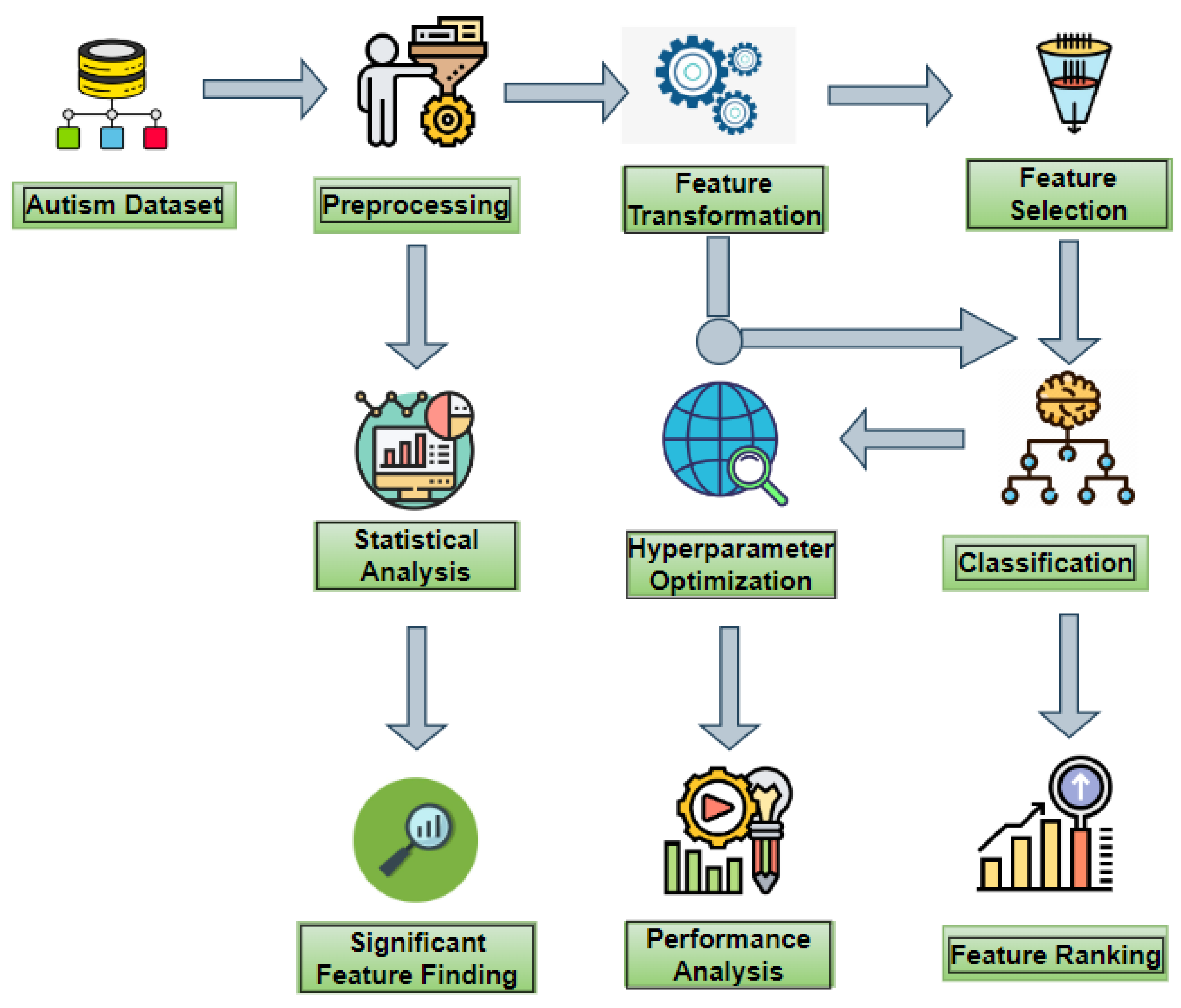
2. Materials and Methods

We applied statistical and machine-learning techniques to an ASD dataset. In the preprocessing step, we converted categorical data to numeric data and utilized the SMOTE technique to balance the dataset. Following this, we utilized Standard Scalar Transformation, Unit Vector Transformation, Robust Scalar Transformation, and Yeo-Johnson Transformation feature transformation models to determine which data was most suitable for machine learning algorithms. Then, we adopted the Recursive Feature Elimination, Pearson Correlation Coefficient, Mutual Information Gain, and Boruta models for feature selection to detect autism spectrum disorder at an early stage. We used Decision tree, Extreme gradient boosting, AdaBoost, Support vector machine, K-Nearest Neighbor, Multilayer perceptron, Gradient boosting, Naive Bayes, Random Forest, and Logistic Regression to identify ASD during the classification step. The grid search method was then used to optimize hyperparameters for optimal performance. Lastly, ML algorithms and Chi-square test were used to determine the most important factor responsible for ASD. Figure 1 depicts a graphical representation of this task.

2.1. Dataset

This data collection covers Autism screening results for toddlers (ages 12 to 36 months). The dataset has been obtained from Kaggle [15] and there are 506 samples in the data set, 346 of which are autistic and 160 of which are normal. Using an online questionnaire in Google Forms, data is collected. The questionnaire consists of Q-CHAT-10 questions in addition to age, gender, area, and family history of autism spectrum disorder (ASD). For question number A1 and A7, the possible responses are leveled as 1 for always, 2 for usually, 3 for sometimes, 4 for rarely, and 5 for never. In contrast, for question number A2, the possible responses are very easy, quite easy, quite difficult, very difficult, and impossible. Many times per day, a few times per day, a few times per week, less than once per week, or never were the possible responses for questions A3, A4, A5, A6, A9, and A10. For question A8, the responses were very typical, quite typical, slightly unusual, and extremely unusual, and my child does not communicate. If the answer to a question from A1 to A9 is the third, fourth, or fifth response, the number 1 is submitted. For A10, the first, second, or third place answer receives the value 1. If the child scores 3 or more on each of the 10 questions, the child may have ASD; otherwise, the child does not have ASD. The details of the dataset are displayed in

Table 1. Dataset Description.

	Feature	Type	Values/Count/Statistics	Description
1	Does your child look at you when youcall his/her name (A1)?	Categorical	Yes = 285 No = 221	Yes, No
2	How easy is it for you to get eye contact with your child (A2)?	Categorical	Yes = 247 No = 259	Yes, No
3	Does your child point to indicate that s/he wants something (A3)?	Categorical	Yes = 259 No = 247	Yes, No
4	Does your child point to share interest with you (A4)?	Categorical	Yes = 266 No = 240	Yes, No
5	Does your child pretend (A5)? (e.g., care for dolls‚ talk on a toy phone)	Categorical	Yes = 283 No = 223	Yes, No
6	Does your child follow where you’re looking (A6)?	Categorical	Yes = 278 No = 228	Yes, No
7	If you or someone else in the family is visibly upset‚ does your child show signs of wanting to comfort them (A7)?	Categorical	Yes = 280 No = 226	Yes, No
8	Would you describe your child’s first words as (A8):	Categorical	Yes = 291 No = 215	Yes, No
9	Does your child use simple gestures (A9)? (e.g., wave goodbye)	Categorical	Yes = 275 No = 231	Yes, No
10	Does your child stare at nothing with no apparent purpose (A10)?	Categorical	Yes = 314 No = 192	Yes, No
11	Region	Categorical	Al Baha = 7 Najran = 9, Tabuk = 18 Jizan = 19 Makkah = 217 Northern Borders = 15 Aseer = 13 Riyadh = 85 Ha’il = 16 Madinah = 23 Eastern = 50 Al Jawf = 12 Qassim = 22	List of regions
12	Age	Number	Mean = 24.445, Standard deviation = 8.35	Toddlers (Months)
13	Gender	Categorical	Female = 349 Male = 157	Male or Female
14	Screening Score	Number	Mean = 5.49, Standard deviation = 3.18	From 1 to 10
15	Family member with ASD history	Boolean	Yes = 122 No = 384	Family members has ASD traits or not
16	Who is completing test	Categorical	Family member = 414 Other = 92	Parents or other
17	Class	Boolean	ASD = 346 No ASD = 160	No ASD traits or ASD traits

. The correlation of each feature is shown in Figure 2. Since there is a strong association with the Screening Score trait, we eliminate this feature.

2.2. Dataset Balancing Technique

Because of its simplicity, SMOTE was utilized to address the issue of class label imbalance and it may be viewed as an improved kind of resampling. It adjusts the minority class by generating additional synthetic samples of the same quality as the class label, hence balancing the category trait. This raises the size of the sample, yet balances the class, providing a resampled range of data for the study. Employing Python’s imblearn module, we finally generated the dynamically resampled data set [16].

2.3. Feature Transformation Method

Feature transformation uses a mathematical formula to change data in a column (feature) for further investigation. It improves prediction accuracy. There are several sorts of feature transformation techniques, such as standard Scalar Transformation (SST), Unit Vector Transformation (UVT), Robust Scalar Transformation (RS), and Yeo-Johnson Transformation (YJT).

Standard Scalar Transformation is employed when input dataset characteristics have vast ranges or are measured in multiple units like Height, Weight, Meters, Miles, etc. We normalize all characteristics so that the mean is 0 and the standard deviation is 1. It subtracts attribute values by their average and divides by standard deviation, resulting in standard normal distribution [17].

In Unit Vector Scalar/Normalizer, the process of normalization involves scaling the values of the individual samples so that they have a unit norm [18]. The most intriguing aspect is that, in contrast to the other scalers, which operate on the values of each particular column, the Normalizer operates on the rows. Each row of the data frame that has at least one non-zero component is separately rescaled to ensure that its norm is equal to one after the rescaling process.

The robust scalar method [18] is another feature transformation method. When we perform the scaling process with constant values (mean, maximum value, etc.), the procedure becomes susceptible to outlier values. When there are several extreme values present in the data, scaling across the interquartile range (IQR) can produce a distribution that is more reliable. The data are normalized based on a median of 0 and are scaled accordingly.

When there is heteroskedasticity, which is a problem with linear connections, power transformation is a technique that may be utilized. It indicates that the standard deviation of the residuals is not a fixed value. The data become more Gaussian after undergoing power transformation. These techniques make use of data known as lambda as a parameter. This parameter contributes to lowering the skewness and maintaining the variance of the data. If the data in the power transformation technique contains zero or negative values, it is called Yeo-Johnson Transformation [19].

2.4. Feature Selection Method

It is essential to recognize key characteristics in order to diagnose ASD. In our research, we have employed four feature selection strategies. The recursive feature elimination technique is the most effective among them.

• Recursive Feature Elimination: Recursive feature elimination [20], often known as RFE, is a method for selecting features that fits a model and removing the weakest feature (or features) one by one until the necessary number of features has been attained.
• Pearson Correlation Coefficient: A value between −1 and 1 known as a Pearson correlation [21] describes the degree to which two variables are linearly connected. The “product-moment correlation coefficient” (PMCC) or simply “correlation” are other names for the Pearson correlation. Only metric variables are appropriate for Pearson correlations. Values for the correlation coefficient range from −1 to 1. A number that is nearer 0 indicates a weaker association (exact 0 implying no correlation). Values closer to 1 indicate a stronger positive association. A number nearer to −1 denotes a more significant negative correlation metric parameter.
• Mutual Information Gain: Evaluation of the information gain contributed by each variable in relation to the target variable is one method for using information gain in the context of feature selection [22]. When used in this context, the calculation is referred to as the mutual information between the two random variables.
• Boruta: The random forest classification method is the core of the Boruta feature selection algorithm, which is a wrapper constructed around it [23]. It makes an effort to identify all of the significant and intriguing characteristics that our dataset may include in relation to a certain outcome variable. First, it will make a copy of the dataset and then it will randomly reorder the numbers in each column.

2.5. Statistical Analysis

The Chi-square test uses the p value to measure the importance of a feature connected to the predictor variables. If the p value is above 0.05, then the category characteristics do not correlate with the dependent variable of interest. The existence of a correlation between the category features and the dependent variable can be inferred if the p-value is below 0.05. Then, we pick the best characteristics to use in our ASD detection algorithm [24,25].

2.6. Machine Learning Model

In our research, we utilized Decision Tree, Extreme Gradient Boosting, Ada Boosting, Support Vector Machine, K-Nearest Neighbor, Multilayer Perceptron, Gradient Boosting, Naive Bayes, Random Forest, and Logistic Regression machine learning techniques. In our dataset, we have tabular labelled data, so supervised machine learning algorithms are suitable for analysis. We have used clinically applicable supervised ML algorithms with model tuning, feature selection, and various optimizations to achieve better evaluation scores. Their descriptions are provided below.

A decision tree (DT) is a classifier model used to identify the category to which a test sample belongs. The DT grows its nodes by optimizing information acquisition at each stage. A single tree is prone to overfitting while having good interpretability. In order to address the overfitting problem of the decision tree [26] algorithm, RF built a number of simple trees to train a dataset of random features on a random subset of observations. The majority of these trees’ decisions will be used to classify a test sample.

Extreme Gradient Boosting (XGBoost) is a well-known technique of supervised learning that is conceivable for huge datasets for the purposes of regression and classification. XGBoost [27] is an integrated model that makes use of a gradient boost framework and is based on the scalable tree boosting system. Its primary goals are to enhance performance and speed.

AdaBoost (AB) is a classifier using ensemble boosting which was proposed by Yoav Freund and Robert Schapire in 1996. A boosted classifier has the following form

$$A_T\left(x\right)=\sum _{t=1}^T{a}_t\left(x\right)$$

(1)

where each $a_t$ is a weak learner that accepts an object x as input and returns a value indicating the object’s class. It improves the accuracy of the classifiers by combining multiple weak classifiers. In order to create a powerful classifier with high accuracy, the AdaBoost classifier [28] combines several weak classifiers. AdaBoost should adhere to two requirements: On varied weighted training instances, the classifier should be trained interactively. It makes an effort to minimize training errors with each iteration in order to offer a perfect match for these samples.

A Support Vector Machine (SVM) is one of the supervised learning models, which takes as input a set of labelled training samples and outputs an ideal hyperplane in n-dimensional space [29]. In support vector machines, a training set is needed to understand the distinctions between the two groups, and a test set is also needed to assess how well the classification performed on previously unexplored data. SVM may be utilized in either a linear or nonlinear fashion in order to distinguish the data that can be separated. Non-linearly separable instances in the input space that could be separated from the right mapping onto a higher-dimensional function space are the ones that are utilized to determine which kernel strategies should be used.

In the field of image processing, the K-Nearest Neighbor (K-NN) algorithm [30] may be used in a range of situations. The three most important aspects of this algorithm are a list of training examples that have been labelled, and a measurement that establishes a distance between the test set and the training set’s example. The value of k is the number of examples that are the test set’s nearest neighbours. These are the three most important aspects. We define test set instances from the two classes that may be mathematically stated as using metrics such as Euclidean distance (ED), Riemannian distance (RD), and others.

$$ED=\sqrt{\left(\sum _{i=1}^4{\left(a_i-b_i\right)}^2\right)}$$

(2)

$$RD=∥log{a}_i^{-1}{b}_i∥$$

(3)

The multilayer perceptron, often known as MLP, is a kind of artificial neural network that uses feedforward connections and translates input data sets to outputs that are more suitable. A Multi-layered Perceptron (MLP) [31] consists of numerous levels, each of which is completely related to the layer that comes after it. With the exception of the nodes that make up the input layer, the neurons that make up the nodes of the layers have nonlinear activation functions. It is possible that there are one or more nonlinear hidden layers located between the input layer and the output layer. The capability to learn non-linear models is the advantage of MLP. The disadvantage of MLP is that its hidden layers have a non-convex loss function where there exists more than one local minimum. A variety of hyperparameters, including the number of hidden neurons, layers, and iterations, must be tuned for MLP.

There is a type of machine learning algorithm known as a Gradient Boosting (GB) classifier. These classifiers take several less capable learning models and integrate them into one robust prediction model. In the practice of gradient boosting, decision trees are frequently utilized. GB [32] provides a prediction model in the form of a collection of decision trees-like weak prediction models. GB trees are the name of the resultant method when a decision tree acts as the weak learner.

The Naive Bayes (NB) [13] method provides a test sample that is determined by the likelihood of the highest class. It is almost immune to the effects of artificial oversampling, and the greatest results are achieved when the method is not used (oversampling of 0%). Within the context of this investigation, we advocated for the application of kernel density estimation in order to get more accurate estimations of the pdf properties. The findings, on the other hand, were only somewhat less favourable than they would have been with the standard Gaussian assumption. Regarding achieving a consistent model of categorization, the Naive Bayes algorithm obtained one of the best outcomes. In addition to this, the goal is to get the best possible AUC. It is important to note that even though there was no need for oversampling when the whole feature selection was performed, the ideal scenario after feature selection was still able to be attained following artificial ASD instance multiplication.

Random Forest (RF) is one kind of decision tree in which the output class of the ensemble is the decision trees’ separate output classes’ style of operation [33]. It is a method that uses an ensemble of models and focuses on the variation in the overall error term. The fundamental concept underlying RF is to bring down the variance term while maintaining the bias’s consistency and bringing the overall error of the ensemble down to a lower value. The classifiers that have a significant use of a decision tree are multiplied in order to attain this goal of minimizing the variance. The comparison of the DT is an effective method for reducing or eliminating mistakes, and the more sophisticated or uncorrelated the trees are, the more effective this method is. The use of unnamed data is accomplished by the use of data processing, which involves the construction of decision trees. Each tree is trained using a copy of the bootstrap data, which was produced using a random sampling procedure and original data replacement.

Logistic Regression (LR) is a form of supervised learning in which the likelihood of a target variable is predicted. Due to the fact that the goal or purpose of the dependent variable is dichotomous, there are two alternative groupings. The dependent variable may be thought of as a binary variable, with the data being recorded as either 1 (which represents success/yes) or 0 (which represents failure/no) [34].

2.7. Hyperparameter Optimization Technique

Grid Search (GS) is a commonly used hyperparameter optimization technique. GS is capable of adjusting the features in accordance with the scale factor inside the defined range of parameters [35]. To determine the attribute with the maximum accuracy, the classifier is trained using the changed parameters. This whole procedure is a cycle, and the comparisons are repeated within the cycle.

2.8. Performance Evaluation Metrics

The effectiveness of all suggested frameworks on ASD datasets were measured mathematically. The following equations are used to figure out the Accuracy (A) [36], Kappa Statistics (KS) [37], Precision (P) [38], Recall (R) [39], AUROC [40], F1-score (F1) [36], and Log loss (LL) [41]:

$$A=(TP+TN)/n$$

(4)

$$KS=\frac{1-(1-p_0)}{1-p_e}$$

(5)

$$P=\frac{TP}{TP+FP}$$

(6)

$$R=\frac{TP}{TP+FN}$$

(7)

$$F1=2\frac{R\ast P}{R+P}$$

(8)

$$TPR=\frac{TP}{TP+FN}$$

(9)

$$FPR=\frac{FP}{FP+FN}$$

(10)

$$LL=-1.0\ast \left(ylog\left(y^{\prime }\right)\right)+(1-y)\ast log\left(1-y^{\prime }\right)$$

(11)

Here, True Positive (TP) indicates that an ASD sample was appropriately identified as having ASD. True Negative (TN) denotes a non-ASD sample that was accurately predicted to be non-ASD. False Positive (FP) indicates that ASD data was incorrectly identified as Non-ASD data. False Negative (FN) samples are non-ASD samples that were incorrectly classified as ASD samples. The sum of all samples is n. The real value is y and the anticipated possibility is $y^{\prime }$. In the Kappa-Statistics $p_0$ is among the raters agreement of relative observation, and $p_e$ is the chance agreement for hypothetical probability.

3. Results

In our work, we implemented a variety of machine-learning classifiers, including DT, NB, KNN, RF, GB, XGB, MLP, SVM, AB, and LR. The experimental work was done at Google Colaboratory using sci-kit-learn in Python. A 10-fold cross-validation approach [42] is applied in this study to develop prediction models. The datasets are arbitrarily split into equivalent 10-fold using the 10-fold cross-validation method. At the time of model construction, nine folds are employed for training, and one is utilized for testing. This technique is repeated 10 times, and the outcomes are then averaged. To validate the experiment results, various assessment metrics, such as accuracy, kappa statistics, precision, recall, AUROC, F1-score, and log loss are analyzed.

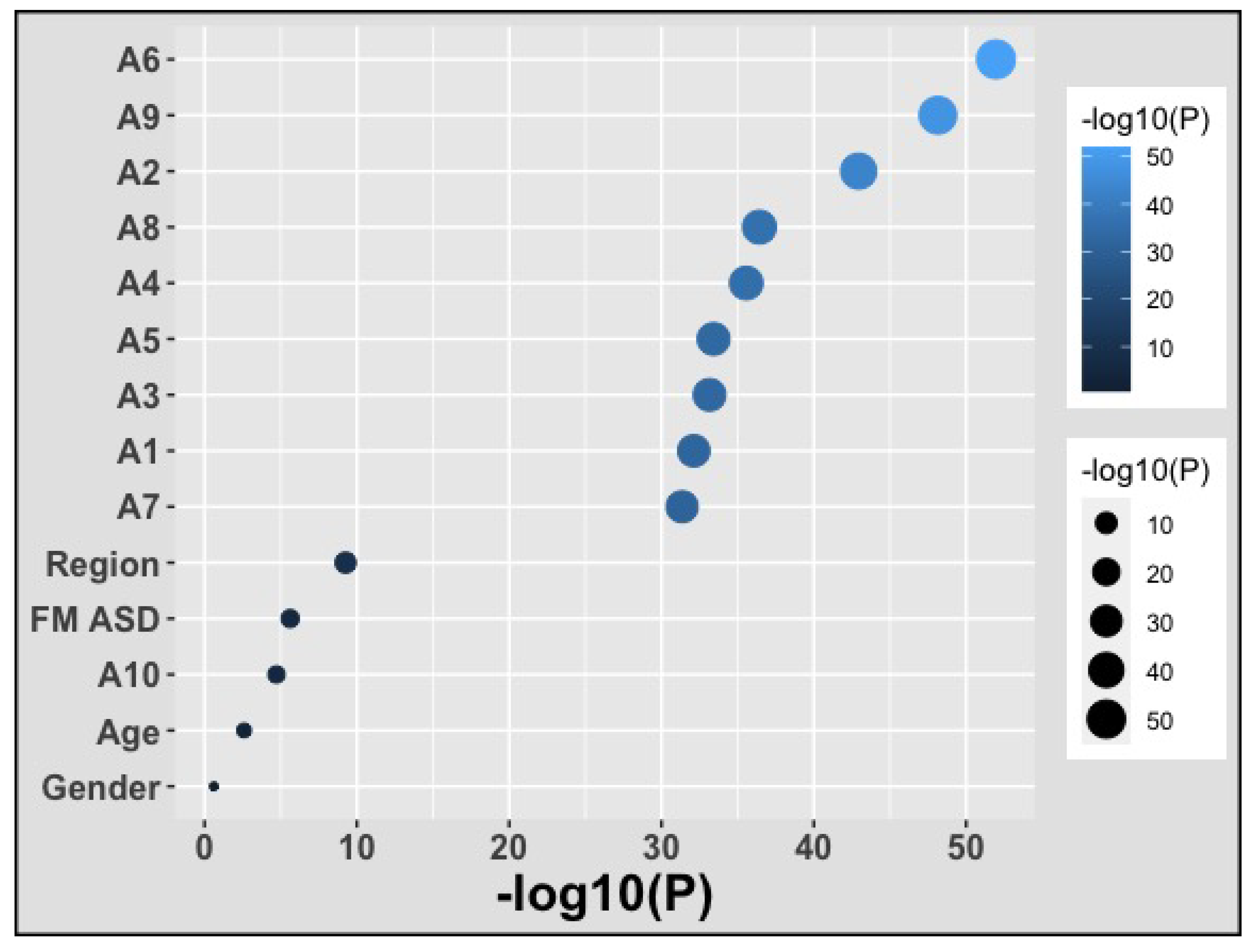
3.1. Finding Significantly Associative Features Using Statistical Methods

We applied the Chi-square test to the ASD dataset in order to detect the most influential causes of autism disorder. Our result is depicted in Figure 3. We find that A6, A9, A2, A8, and A4 are the most important qualities, whereas Gender, Age, A10, FM ASD, and Region are the least important ones.

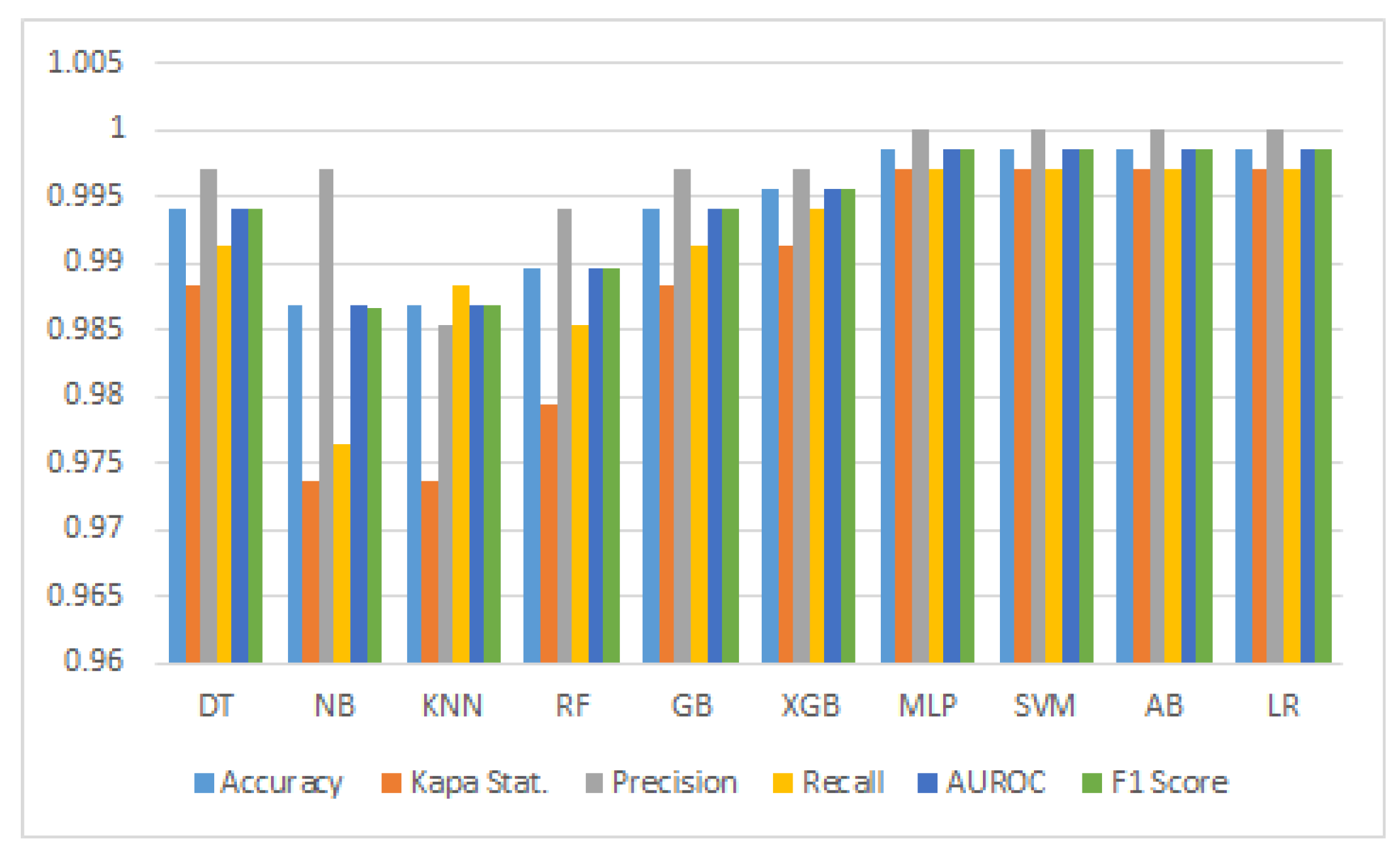
3.2. Analysis of Accuracy

The result of accuracy for each classifier is shown in

Table 2. Performance Analysis of Different Classifiers in the Main and Balanced Dataset.

EM	Dataset	DT	NB	KNN	RF	GB	XGB	MLP	SVM	AB	LR
Accuracy	Main	0.9407	0.9506	0.8992	0.9585	0.9664	0.9743	0.9704	0.8854	0.9941	0.9901
	Balanced	0.9545	0.9428	0.9223	0.9633	0.9707	0.978	0.9692	0.937	0.9956	0.9912
Kapa Stat.	Main	0.8643	0.886	0.778	0.9051	0.9232	0.9415	0.9329	0.7342	0.9866	0.9777
	Balanced	0.9091	0.8856	0.8446	0.9267	0.9413	0.956	0.9384	0.8739	0.9912	0.9824
Precision	Main	0.9507	0.9514	0.9531	0.9651	0.9709	0.9795	0.9822	0.9008	1.000	1.000
	Balanced	0.9613	0.9016	0.9706	0.954	0.9679	0.9766	0.9678	0.9776	1.000	1.000
Recall	Main	0.9619	0.9765	0.8944	0.9736	0.9795	0.9824	0.9736	0.9326	0.9912	0.9853
	Balanced	0.9472	0.9941	0.871	0.9736	0.9736	0.9795	0.9707	0.8944	0.9912	0.9824
AUC-ROC	Main	0.9294	0.9368	0.9018	0.9504	0.9594	0.97	0.9686	0.8602	0.9956	0.9927
	Balanced	0.9545	0.9428	0.9223	0.9633	0.9707	0.978	0.9692	0.937	0.9956	0.9912
F1 score	Main	0.9563	0.9638	0.9228	0.9693	0.9752	0.981	0.9779	0.9164	0.9956	0.9926
	Balanced	0.9542	0.9456	0.9181	0.9637	0.9708	0.978	0.9693	0.9342	0.9956	0.9911
Log loss	Main	2.0478	1.7065	3.4812	1.4334	1.1604	0.8874	1.0239	3.959	0.2048	0.3413
	Balanced	1.57	1.9751	2.6841	1.2661	1.0129	0.7597	1.0635	2.1777	0.1519	0.3039

The bold text indicates the highest values.

,

Table 3. Analysis of the Performance of Different Classifiers Based on Varied Feature Transformation Techniques.

EM	Dataset	DT	NB	KNN	RF	GB	XGB	MLP	SVM	AB	LR
Accuracy	Standard Scalar	0.9589	0.9428	0.9663	0.9663	0.9765	0.9809	0.9941	0.9795	0.9985	0.9956
	Unit Vector	0.9428	0.9267	0.9575	0.9663	0.9677	0.9736	0.9428	0.9238	0.9897	0.8314
	Yeo-Johnson	0.9604	0.9428	0.9663	0.9736	0.9721	0.978	0.9941	0.9824	0.9941	0.9956
	Robust Scalar	0.9633	0.9428	0.9575	0.9692	0.9736	0.9809	0.9927	0.9795	0.9985	0.9941
Kapa Stat.	Standard Scalar	0.9179	0.8856	0.9326	0.9326	0.9531	0.9619	0.9883	0.9589	0.9971	0.9912
	Unit Vector	0.8856	0.8534	0.915	0.9326	0.9355	0.9472	0.8856	0.8475	0.9795	0.6628
	Yeo-Johnson	0.9208	0.8856	0.9326	0.9472	0.9443	0.956	0.9883	0.9648	0.9883	0.9912
	Robust scalar	0.9267	0.8856	0.915	0.9384	0.9472	0.9619	0.9853	0.9589	0.9971	0.9883
Precision	Standard Scalar	0.9672	0.9016	0.9877	0.9543	0.971	0.9795	1.0000	0.9712	1.0000	1.0000
	Unit Vector	0.9415	0.9076	0.9588	0.9543	0.9544	0.9681	0.9415	0.9446	0.9912	0.8717
	Yeo-Johnson	0.9673	0.9016	0.9969	0.9654	0.9708	0.9766	0.9971	0.9768	1.0000	1.0000
	Robust scalar	0.9731	0.9016	0.9937	0.9598	0.9681	0.9795	0.9941	0.9767	1.0000	1.0000
Recall	Standard Scalar	0.9501	0.9941	0.9443	0.9795	0.9824	0.9824	0.9883	0.9883	0.9971	0.9912
	Unit Vector	0.9443	0.9501	0.956	0.9795	0.9824	0.9795	0.9443	0.9003	0.9883	0.7771
	Yeo-Johnson	0.9531	0.9941	0.9355	0.9824	0.9736	0.9795	0.9912	0.9883	0.9883	0.9912
	Robust scalar	0.9531	0.9941	0.9208	0.9795	0.9795	0.9824	0.9912	0.9824	0.9971	0.9883
AUC-ROC	SST	0.9589	0.9428	0.9663	0.9663	0.9765	0.9809	0.9941	0.9795	0.9985	0.9956
	Unit Vector	0.9428	0.9267	0.9575	0.9663	0.9677	0.9736	0.9428	0.9238	0.9897	0.8314
	Yeo-Johnson	0.9604	0.9428	0.9663	0.9736	0.9721	0.978	0.9941	0.9824	0.9941	0.9956
	Robust scalar	0.9633	0.9428	0.9575	0.9692	0.9736	0.9809	0.9927	0.9795	0.9985	0.9941
F1 score	Standard Scalar	0.9586	0.9456	0.9655	0.9667	0.9767	0.981	0.9941	0.9797	0.9985	0.9956
	Unit Vector	0.9429	0.9284	0.9574	0.9667	0.9682	0.9738	0.9429	0.9219	0.9897	0.8217
	Yeo-Johnson	0.9601	0.9456	0.9652	0.9738	0.9722	0.978	0.9941	0.9825	0.9941	0.9956
	Robust scalar	0.963	0.9456	0.9559	0.9695	0.9738	0.981	0.9927	0.9795	0.9985	0.9941
Log loss	Standard Scalar	1.418	1.9751	1.1648	1.1648	0.8103	0.6584	0.2026	0.709	0.0506	0.1519
	Unit Vector	1.9751	2.5322	1.4687	1.1648	1.1142	0.9116	1.9751	2.6335	0.3545	5.824
	Yeo-Johnson	1.3674	1.9751	1.1648	0.9116	0.9622	0.7597	0.2026	0.6077	0.2026	0.1519
	Robust scalar	1.2661	1.9751	1.4687	1.0635	0.9116	0.6584	0.2532	0.709	0.0506	0.2026

The bold text indicates the highest values.

,

Table 4. Evaluation of the Performance of Different Classifiers Employing Varied Feature Selection Methods.

EM	Feature Selection Technique	DT	NB	KNN	RF	GB	XGB	MLP	SVM	AB	LR
Accuracy	Boruta	0.9604	0.9428	0.9677	0.9648	0.9707	0.9721	0.9765	0.9721	0.9765	0.9765
	Pearson Correlation Coefficient	0.9633	0.9501	0.9604	0.9736	0.9707	0.9692	0.9751	0.9677	0.9765	0.9736
	Mutual Information Gain	0.9648	0.9531	0.9604	0.9721	0.9824	0.9839	0.9941	0.9927	0.9956	0.9956
	Recursive Feature Elimination	0.9721	0.9457	0.9663	0.9736	0.9839	0.9839	0.9956	0.9839	0.9956	0.9956
Kapa Stat.	Boruta	0.9208	0.8856	0.9355	0.9296	0.9413	0.9443	0.9531	0.9443	0.9531	0.9531
	Pearson Correlation Coefficient	0.9267	0.9003	0.9208	0.9472	0.9413	0.9384	0.9501	0.9355	0.9531	0.9472
	Mutual Information Gain	0.9296	0.9062	0.9208	0.9443	0.9648	0.9677	0.9883	0.9853	0.9912	0.9912
	Recursive Feature Elimination	0.9443	0.8915	0.9326	0.9472	0.9677	0.9677	0.9912	0.9677	0.9912	0.9912
Precision	Boruta	0.9701	0.9016	0.9878	0.9621	0.9707	0.9763	0.9794	0.9708	0.9794	0.9765
	Pearson Correlation Coefficient	0.9675	0.9183	0.9846	0.9681	0.9707	0.9678	0.9737	0.9623	0.9765	0.9792
	Mutual Information Gain	0.9648	0.921	0.9968	0.9653	0.9853	0.9882	1.0000	0.9941	1.0000	1.0000
	Recursive Feature Elimination	0.9735	0.9086	0.9938	0.9681	0.9882	0.9853	1.0000	0.9882	1.0000	1.0000
Recall	Boruta	0.9501	0.9941	0.9472	0.9677	0.9707	0.9677	0.9736	0.9736	0.9736	0.9765
	Pearson Correlation Coefficient	0.9589	0.9883	0.9355	0.9795	0.9707	0.9707	0.9765	0.9736	0.9765	0.9677
	Mutual Information Gain	0.9648	0.9912	0.9238	0.9795	0.9795	0.9795	0.9883	0.9912	0.9912	0.9912
	Recursive Feature Elimination	0.9707	0.9912	0.9384	0.9795	0.9795	0.9824	0.9912	0.9795	0.9912	0.9912
AUC-ROC	Boruta	0.9604	0.9428	0.9677	0.9648	0.9707	0.9721	0.9765	0.9721	0.9765	0.9765
	Pearson Correlation Coefficient	0.9633	0.9501	0.9604	0.9736	0.9707	0.9692	0.9751	0.9677	0.9765	0.9736
	Mutual Information Gain	0.9648	0.9531	0.9604	0.9721	0.9824	0.9839	0.9941	0.9927	0.9956	0.9956
	Recursive Feature Elimination	0.9721	0.9457	0.9663	0.9736	0.9839	0.9839	0.9956	0.9839	0.9956	0.9956
F1 score	Boruta	0.96	0.9456	0.9671	0.9649	0.9707	0.972	0.9765	0.9722	0.9765	0.9765
	Pearson Correlation Coefficient	0.9632	0.952	0.9594	0.9738	0.9707	0.9693	0.9751	0.9679	0.9765	0.9735
	Mutual Information Gain	0.9648	0.9548	0.9589	0.9723	0.9824	0.9838	0.9941	0.9927	0.9956	0.9956
	Recursive Feature Elimination	0.9721	0.9481	0.9653	0.9738	0.9838	0.9838	0.9956	0.9838	0.9956	0.9956
Log loss	Boruta	1.3674	1.9751	1.1142	1.2155	1.0129	0.9622	0.8103	0.9622	0.8103	0.8103
	Pearson Correlation Coefficient	1.2661	1.7219	1.3674	0.9116	1.0129	1.0635	0.8609	1.1142	0.8103	0.9116
	Mutual Information Gain	1.2155	1.6206	1.3674	0.9622	0.6077	0.5571	0.2026	0.2532	0.1519	0.1519
	Recursive Feature Elimination	0.9622	1.8738	1.1648	0.9116	0.5571	0.5571	0.1519	0.5571	0.1519	0.1519

The bold text indicates the highest values.

and

Table 5. Performance Analysis of Several Classifiers Using Grid Search Technique.

Classifier	DT	NB	KNN	RF	GB	XGB	MLP	SVM	AB	LR
Accuracy	0.9941	0.9868	0.9868	0.9897	0.9941	0.9956	0.9985	0.9985	0.9985	0.9985
Kapa Stat.	0.9883	0.9736	0.9736	0.9795	0.9883	0.9912	0.9971	0.9971	0.9971	0.9971
Precision	0.9971	0.997	0.9854	0.9941	0.9971	0.9971	1.000	1.000	1.000	1.000
Recall	0.9912	0.9765	0.9883	0.9853	0.9912	0.9941	0.9971	0.9971	0.9971	0.9971
AUC-ROC	0.9941	0.9868	0.9868	0.9897	0.9941	0.9956	0.9985	0.9985	0.9985	0.9985
F1 Score	0.9941	0.9867	0.9868	0.9897	0.9941	0.9956	0.9985	0.9985	0.9985	0.9985
Log Loss	0.2026	0.4558	0.4558	0.3545	0.2026	0.1519	0.0506	0.0506	0.0506	0.0506

The bold text indicates the highest values.

. AB calculated the maximum accuracy for the main and balanced datasets (99.41% and 99.56%, respectively). When we investigated the FS approach, the MLP, AB, and LR in recursive feature elimination technique and the AB and LR in the mutual information gain method produced the results with the highest accuracy (99.56%). The maximum accuracy (99.85%) was calculated by AB in both standard scalar and robust scalar FT methods. After hyperparameter adjustment for each classifier, MLP, SVM, AB, and LR produced the most accurate results, 99.85%.

In this study, we also observed that AB provided the best results among all classifiers for the mutual information gain and recursive feature elimination FS methods, the standard scalar and robust scalar FT methods, and the hyperparameter optimization methodology.

3.3. Result Analysis of Kappa Statistics

Each classifier’s kappa statistics (KP) values are shown in Table 2, Table 3, Table 4 and Table 5. The AB produced the highest scores for both the main dataset and the balanced dataset, which were 98.66% and 99.12%, respectively. It has been observed that the balanced dataset performed better than the main dataset. AB and LR estimated the highest results (99.12%) for the mutual information gain and recursive feature elimination techniques, whilst MLP evaluated the best result by using the recursive feature elimination methodology. AB calculated the maximum outcome for standard scalar and robust scalar approaches in the FT technique. For the hyperparameter tuning approach, MLP, SVM, AB, and LR determined the highest possible result, which was 99.71%.

3.4. Analysis of Precision

Table 2, Table 3, Table 4 and Table 5 display the precision value of each classifier. AB and LR manipulated the maximum outcome in the case of main dataset and balanced dataset. When we observed the FS method, the highest precision value was determined by MLP, AB, and LR for both mutual information gain and recursive feature elimination methods. The MLP, AB, and LR calculated the maximum results for standard scalar in the FT method. The LR and AB evaluated the highest result for both Yeo-Johnson and robust scalar techniques. The highest result (100%) was generated by MLP, SVM, AB, and LR in the case of parameter tuning.

3.5. Analysis of Recall

The recall results for each classifier are displayed in Table 2, Table 3, Table 4 and Table 5, respectively. AB calculated the highest recall value (99.12%) for the primary dataset, whereas NB produced the best result (99.41%) for the balanced dataset. When we investigated the FS method, the NB produced the highest boruta result of 99.41%. AB calculated the maximum recall (99.71%) using both the standard scalar and robust scalar FT methods. After tuning the hyperparameters for each classifier, MLP, SVM, AB, and LR provided the highest result, 99.71%. Finally, it is found that, among all classifiers, the AB classifier performed the best.

3.6. Analysis of AUROC

Table 2, Table 3, Table 4 and Table 5 display the AUROC values for each classifier. The AB gave the greatest main dataset and balanced dataset scores, both of which were 99.56%. AB and LR estimated the highest results (99.56%) for the mutual information gain and recursive feature elimination methods, whereas MLP calculated the same result using the recursive feature elimination technique. AB calculated the best results for the standard scalar and robust scalar techniques in the FT methodology. In the case of the hyperparameter tuning method, MLP, SVM, AB, and LR determined the highest achievable outcome, which was 99.85%. After hyperparameter adjustment, it is observed that the performance of each classifier is enhanced.

3.7. Analysis of F1 Score

Table 2, Table 3, Table 4 and Table 5 list the F1 score of each classifier. AB manipulated the maximum result for main dataset and balanced dataset, which was 99.56%. MLP, AB, and LR for recursive feature elimination methods found the greatest F1 score value when we observed the FS method. In contrast, AB and LR calculated the maximum result for mutual information gain technique. In case of FT techniques, the AB determined that the standard scalar and robust scalar techniques produced the best results. In terms of parameter tuning, MLP, SVM, AB, and LR produced the maximum accuracy (99.85%).

3.8. Analysis of Log loss

The log loss results for each classifier are displayed in Table 2, Table 3, Table 4 and Table 5. AB estimated the least amount of log loss for the primary and balanced datasets (20.48% and 15.19%, respectively). The MLP, AB, and LR in recursive feature elimination technique and the AB and LR in the mutual information gain method yielded the lowest results (15.19%) when we examined the FS method. AB calculated the lowest (5.06%) using both the standard scalar and robust scalar FT methods. After adjusting each classifier’s hyperparameters, MLP, SVM, AB, and LR yielded the lowest log loss (5.06%) which is shown in Figure 4. In this investigation, we also found that AB offered the best results among all classifiers for all feature transformation and selection techniques, as well as the hyperparameter optimization strategy. The performance of different classifiers using the hyperparameter optimization technique is demonstrated in Figure 5. Here, we observed that MLP, SVM, AB, and LR demonstrated the best outcome.

3.9. Feature Ranking Using Machine Learning Technique

We calculated feature importance using the average coefficient value of all used classifiers. We evaluate attribute significance values for each approach, and then balanced them using the standard scalar technique so that they fall between 0 and 1. We then calculated averages across all dimensions. In

Table 6. Feature Ranking Using Machine Learning Technique based on coefficient values.

Feature	DT	NB	KNN	RF	GB	XGB	MLP	SVM	AB	LR	Average
A10	0.039	0.000	0.325	0.380	0.319	0.353	0.687	0.101	0.833	0.107	0.314
A9	0.135	0.016	0.662	0.155	0.028	0.073	0.707	0.815	0.833	0.803	0.423
A8	0.036	1.000	0.587	1.000	1.000	1.000	0.867	0.135	0.833	0.148	0.661
A7	0.017	0.674	0.238	0.821	0.521	0.507	0.675	1.000	1.000	1.000	0.645
A6	1.000	0.258	1.000	0.357	0.301	0.484	0.707	0.726	0.667	0.720	0.622
A5	0.050	0.044	0.538	0.004	0.003	0.064	0.663	0.526	0.833	0.507	0.323
A4	0.021	0.052	0.263	0.019	0.018	0.047	0.491	0.542	0.667	0.543	0.266
A3	0.029	0.052	0.238	0.000	0.015	0.000	1.000	0.527	0.833	0.542	0.324
A2	0.280	0.078	0.650	0.159	0.052	0.249	0.809	0.606	0.833	0.590	0.431
A1	0.043	0.721	0.450	0.570	0.267	0.432	0.641	0.431	0.833	0.454	0.484
Region	0.000	0.164	0.000	0.300	0.000	0.043	0.000	0.727	0.167	0.724	0.213
Age	0.011	0.253	0.075	0.526	0.380	0.344	0.203	0.181	0.000	0.178	0.215
Gender	0.026	0.068	0.100	0.013	0.010	0.076	0.110	0.631	0.000	0.657	0.169
FM ASD	0.000	0.661	0.275	0.539	0.165	0.269	0.020	0.000	0.000	0.000	0.193

The bold text indicates highest values of coefficient and most important indicator.

, we found that A8 had the greatest mean coefficient value (0.661) while gender had the lowest mean coefficient value. In Figure 6, we analyzed the relevance of autism’s characteristics and identified A8 as the most prominent. Other critical features are A7, A6, A1, A2, and so on. Gender, FM ASD, Region, Age, A4, A10, etc. are the least essential traits.

4. Discussion

Several studies have been conducted utilizing ASD datasets, although ASD prediction remains in need of substantial improvement. In our research, we collected ASD datasets and balanced them using the SMOTE method. Then, we applied Decision Tree, Naive Bayes, K-Nearest Neighbors, Random Forest, Gradient Boosting, Extreme Gradient Boosting, Multilayer Perceptron, Support Vector Machine, Ada Boost, and Logistic Regression classifiers after transforming the features using various feature transformed techniques, including Standard Scalar, Unit Vector Scalar, Robust Scalar, and Yeo Johnson transformation. All classifiers performed well utilizing the standard scalar approach, with AB achieving the best performance. Subsequently, we applied the feature selection techniques Boruta, Correlation, Mutual Information, and Recursive Feature Elimination, and we achieved good results using the RFE technique. We decreased execution time and memory requirements by utilizing FS to locate ASD as rapidly as feasible. Finally, the grid search hyperparameter optimization technique was implemented. Here, we found that all classifiers improved their performance, with AB, LR, SVM, and MLP producing the best results.

Our results suggest a variety of critical and pertinent features for early diagnosis of ASD. The most important features are A6, A9, A2, A8, and A4 dependent on the log-based relationship. The most important characteristics of an ML model are A8, A7, A6, A1, and A2. In addition, we found significant indicators such as A6, A2, and A8 that are identical for both log-based association and ML methods. Our investigation suggests that key attributes are sufficient for recognizing ASD, which will facilitates the effective application of ASD diagnosis.

The suggested model is contrasted with relevant prior findings in

Table 7. Comparative analysis of the proposed model with the other prior studies.

Reference	Feature Selection	Accuracy	Kapa Stat.	Precision	Recall	AUROC	F1 Score	Log Loss
Akter et al. [14]	No	98.77	97.1			99.98		3.01
Bala et al. [6]	Yes	97.82	94.87			99.7	97.8
Hasan et al. [7]	No	99.25	98.97	99.89	98.45		99.1	0.0802
Proposed Model	Yes	99.85	99.71	1.00	1.00	99.85	99.85	0.0506

. The majority of previous research utilized version-1 ASD datasets, whereas a few studies utilized version-2. Akter et al. utilized the technique of feature transformation and obtained the maximum result accuracy (98.77%), KS (97.1), AUROC (99.98%), and Log Loss (3.01). In a different study, Bala et al. used the feature selection technique and achieved the top results for accuracy (97.82%), KS (94.87), AURCO (99.7%), and F1 Score (97.8). Hasan et al. then performed a feature transformation strategy that yielded the highest accuracy (99.25%), KS (98.97), precision (99.89%), recall (98.45%), F1 Score (99.1%), and Log Loss (0.0802). In our suggested framework, however, the application of feature transformation, selection, and hyperparameter optimization is employed and got the highest accuracy (99.85%), KS (99.71), precision (1.00%), recall (1.00%), AUROC (99.85%), F1 Score (99.85%), and Log Loss (0.0506).

5. Conclusions

In our work, the proposed ML architecture was used to yield more precise and effective results for the rapid diagnosis of ASD. We applied FT techniques to the ASD samples, examined the modified dataset using many classifiers, and evaluated their efficacy. Next, we employed feature extraction strategies to yield fewer characteristics from ASD screening methodologies while preserving performance consistency. In addition, we utilized the hyperparameter optimization method to enhance the performance of each classifier. Our research reveals that the standard scalar feature transformation and RFE feature selection techniques are superior to others.

Our findings may aid in the identification of ASD characteristics, making it easier for patients and their families to gain the necessary support to improve their physical, social, and academic health. This study’s weaknesses include the absence of specific details such as recordings and images of cases and controls. In the future, we will implement deep learning algorithms that enable the discovery of novel, non-conventional ASD traits from a complex set of characteristics. In addition, future research could examine cluster analysis to identify endophenotypes, evaluate the role of development in facilitating evaluation, and improve diagnosis and therapy.

References

1. Crane, L.; Batty, R.; Adeyinka, H.; Goddard, L.; Henry, L.A.; Hill, E.L. Autism diagnosis in the United Kingdom: Perspectives of autistic adults, parents and professionals. J. Autism Dev. Disord. 2018, 48, 3761–3772. [Google Scholar] [CrossRef] [PubMed]
2. Thabtah, F.; Spencer, R.; Abdelhamid, N.; Kamalov, F.; Wentzel, C.; Ye, Y.; Dayara, T. Autism screening: An unsupervised machine learning approach. Health Inf. Sci. Syst. 2022, 10, 26. [Google Scholar] [CrossRef] [PubMed]
3. Thabtah, F.; Kamalov, F.; Rajab, K. A new computational intelligence approach to detect autistic features for autism screening. Int. J. Med. Inform. 2018, 117, 112–124. [Google Scholar] [CrossRef] [PubMed]
4. Thabtah, F.; Abdelhamid, N.; Peebles, D. A machine learning autism classification based on logistic regression analysis. Health Inf. Sci. Syst. 2019, 7, 12. [Google Scholar] [CrossRef] [PubMed]
5. Roccetti, M.; Delnevo, G.; Casini, L.; Mirri, S. An alternative approach to dimension reduction for pareto distributed data: A case study. J. Big Data 2021, 8, 39. [Google Scholar] [CrossRef] [PubMed]
6. Bala, M.; Ali, M.H.; Satu, M.S.; Hasan, K.F.; Moni, M.A. Efficient Machine Learning Models for Early Stage Detection of Autism Spectrum Disorder. Algorithms 2022, 15, 166. [Google Scholar] [CrossRef]
7. Hasan, S.M.; Uddin, M.P.; Al Mamun, M.; Sharif, M.I.; Ulhaq, A.; Krishnamoorthy, G. A Machine Learning Framework for Early-Stage Detection of Autism Spectrum Disorders. IEEE Access 2022, 11, 15038–15057. [Google Scholar] [CrossRef]
8. Rodrigues, I.D.; de Carvalho, E.A.; Santana, C.P.; Bastos, G.S. Machine Learning and rs-fMRI to Identify Potential Brain Regions Associated with Autism Severity. Algorithms 2022, 15, 195. [Google Scholar] [CrossRef]
9. Raj, S.; Masood, S. Analysis and detection of autism spectrum disorder using machine learning techniques. Procedia Comput. Sci. 2020, 167, 994–1004. [Google Scholar] [CrossRef]
10. Hossain, M.D.; Kabir, M.A.; Anwar, A.; Islam, M.Z. Detecting autism spectrum disorder using machine learning techniques. Health Inf. Sci. Syst. 2021, 9, 386. [Google Scholar] [CrossRef]
11. Akter, T.; Shahriare Satu, M.; Khan, M.I.; Ali, M.H.; Uddin, S.; Lió, P.; Quinn, J.M.W.; Moni, M.A. Machine Learning-Based Models for Early Stage Detection of Autism Spectrum Disorders. IEEE Access 2019, 7, 166509–166527. [Google Scholar] [CrossRef]
12. Pietrucci, D.; Teofani, A.; Milanesi, M.; Fosso, B.; Putignani, L.; Messina, F.; Pesole, G.; Desideri, A.; Chillemi, G. Machine Learning Data Analysis Highlights the Role of Parasutterella and Alloprevotella in Autism Spectrum Disorders. Biomedicines 2022, 10, 2028. [Google Scholar] [CrossRef] [PubMed]
13. Omar, K.S.; Mondal, P.; Khan, N.S.; Rizvi, M.R.K.; Islam, M.N. A Machine Learning Approach to Predict Autism Spectrum Disorder. In Proceedings of the 2019 International Conference on Electrical, Computer and Communication Engineering (ECCE), Cox’s Bazar, Bangladesh, 7–9 February 2019; pp. 1–6. [Google Scholar] [CrossRef]
14. Akter, T.; Ali, M.H.; Satu, M.; Khan, M.; Mahmud, M. Towards autism subtype detection through identification of discriminatory factors using machine learning. In International Conference on Brain Informatics; Springer: Cham, Switzerland, 2021; pp. 401–410. [Google Scholar]
15. ASD Screening Data for Toddlers in Saudi. Kaggle. Available online: https://www.kaggle.com/datasets/asdpredictioninsaudi/asd-screening-data-for-toddlers-in-saudi-arabia (accessed on 20 March 2023).
16. Albahri, A.; Hamid, R.A.; Zaidan, A.; Albahri, O. Early automated prediction model for the diagnosis and detection of children with autism spectrum disorders based on effective sociodemographic and family characteristic features. Neural Comput. Appl. 2022, 35, 921–947. [Google Scholar] [CrossRef]
17. Yassin, W.; Nakatani, H.; Zhu, Y.; Kojima, M.; Owada, K.; Kuwabara, H.; Gonoi, W.; Aoki, Y.; Takao, H.; Natsubori, T.; et al. Machine-learning classification using neuroimaging data in schizophrenia, autism, ultra-high risk and first-episode psychosis. Transl. Psychiatry 2020, 10, 278. [Google Scholar] [CrossRef] [PubMed]
18. Ahsan, M.M.; Mahmud, M.P.; Saha, P.K.; Gupta, K.D.; Siddique, Z. Effect of data scaling methods on machine learning algorithms and model performance. Technologies 2021, 9, 52. [Google Scholar] [CrossRef]
19. Zhang, Y.; Yu, Q. What is the best article publishing strategy for early career scientists? Scientometrics 2020, 122, 397–408. [Google Scholar] [CrossRef]
20. Huang, X.; Zhang, L.; Wang, B.; Li, F.; Zhang, Z. Feature clustering based support vector machine recursive feature elimination for gene selection. Appl. Intell. 2018, 48, 594–607. [Google Scholar] [CrossRef]
21. Hu, C.C.; Xu, X.; Xiong, G.L.; Xu, Q.; Zhou, B.R.; Li, C.Y.; Qin, Q.; Liu, C.X.; Li, H.P.; Sun, Y.J.; et al. Alterations in plasma cytokine levels in chinese children with autism spectrum disorder. Autism Res. 2018, 11, 989–999. [Google Scholar] [CrossRef]
22. Battiti, R. Using mutual information for selecting features in supervised neural net learning. IEEE Trans. Neural Netw. 1994, 5, 537–550. [Google Scholar] [CrossRef]
23. Chang, J.M.; Zeng, H.; Han, R.; Chang, Y.M.; Shah, R.; Salafia, C.M.; Newschaffer, C.; Miller, R.K.; Katzman, P.; Moye, J.; et al. Autism risk classification using placental chorionic surface vascular network features. BMC Med. Inform. Decis. Mak. 2017, 17, 162. [Google Scholar] [CrossRef]
24. Belaoued, M.; Mazouzi, S. A real-time pe-malware detection system based on Chi-square test and pe-file features. In Computer Science and Its Applications, Proceedings of the 5th IFIP TC 5 International Conference, CIIA 2015, Saida, Algeria, 20–21 May 2015; Springer: Cham, Switzerland, 2015; pp. 416–425. [Google Scholar]
25. Shrestha, U.; Alsadoon, A.; Prasad, P.; Al Aloussi, S.; Alsadoon, O.H. Supervised machine learning for early predicting the sepsis patient: Modified mean imputation and modified Chi-square feature selection. Multimed. Tools Appl. 2021, 80, 20477–20500. [Google Scholar] [CrossRef]
26. Oh, D.H.; Kim, I.B.; Kim, S.H.; Ahn, D.H. Predicting autism spectrum disorder using blood-based gene expression signatures and machine learning. Clin. Psychopharmacol. Neurosci. 2017, 15, 47. [Google Scholar] [CrossRef] [PubMed]
27. Magboo, V.P.C.; Magboo, M.; Sheila, A. Classification Models for Autism Spectrum Disorder. In International Conference on Artificial Intelligence and Data Science; Springer: Cham, Switzerland, 2022; pp. 452–464. [Google Scholar]
28. Sujatha, R.; Aarthy, S.; Chatterjee, J.; Alaboudi, A.; Jhanjhi, N. A machine learning way to classify autism spectrum disorder. Int. J. Emerg. Technol. Learn. (iJET) 2021, 16, 182–200. [Google Scholar]
29. Retico, A.; Giuliano, A.; Tancredi, R.; Cosenza, A.; Apicella, F.; Narzisi, A.; Biagi, L.; Tosetti, M.; Muratori, F.; Calderoni, S. The effect of gender on the neuroanatomy of children with autism spectrum disorders: A support vector machine case-control study. Mol. Autism 2016, 7, 5. [Google Scholar] [CrossRef] [PubMed]
30. Lohar, M.; Chorage, S. Automatic Classification of Autism Spectrum Disorder (ASD) from Brain MR Images Based on Feature Optimization and Machine Learning. In Proceedings of the 2021 International Conference on Smart Generation Computing, Communication and Networking (SMART GENCON), Pune, India, 29–30 October 2021; pp. 1–7. [Google Scholar] [CrossRef]
31. Negin, F.; Ozyer, B.; Agahian, S.; Kacdioglu, S.; Ozyer, G.T. Vision-assisted recognition of stereotype behaviors for early diagnosis of Autism Spectrum Disorders. Neurocomputing 2021, 446, 145–155. [Google Scholar] [CrossRef]
32. Ismail, E.; Gad, W.; Hashem, M. HEC-ASD: A hybrid ensemble-based classification model for predicting autism spectrum disorder disease genes. BMC Bioinform. 2022, 23, 554. [Google Scholar] [CrossRef]
33. Chen, W.; Xie, X.; Wang, J.; Pradhan, B.; Hong, H.; Bui, D.T.; Duan, Z.; Ma, J. A comparative study of logistic model tree, random forest, and classification and regression tree models for spatial prediction of landslide susceptibility. Catena 2017, 151, 147–160. [Google Scholar] [CrossRef]
34. Li, B.; Sharma, A.; Meng, J.; Purushwalkam, S.; Gowen, E. Applying machine learning to identify autistic adults using imitation: An exploratory study. PLoS ONE 2017, 12, e0182652. [Google Scholar] [CrossRef]
35. Chen, J.; Huang, H.; Cohn, A.G.; Zhang, D.; Zhou, M. Machine learning-based classification of rock discontinuity trace: SMOTE oversampling integrated with GBT ensemble learning. Int. J. Min. Sci. Technol. 2022, 32, 309–322. [Google Scholar] [CrossRef]
36. Akter, T.; Ali, M.H.; Khan, M.I.; Satu, M.S.; Uddin, M.J.; Alyami, S.A.; Ali, S.; Azad, A.; Moni, M.A. Improved transfer-learning-based facial recognition framework to detect autistic children at an early stage. Brain Sci. 2021, 11, 734. [Google Scholar] [CrossRef]
37. Nehm, R.H.; Ha, M.; Mayfield, E. Transforming biology assessment with machine learning: Automated scoring of written evolutionary explanations. J. Sci. Educ. Technol. 2012, 21, 183–196. [Google Scholar] [CrossRef]
38. Ahamad, M.M.; Aktar, S.; Uddin, M.J.; Rahman, T.; Alyami, S.A.; Al-Ashhab, S.; Akhdar, H.F.; Azad, A.; Moni, M.A. Early-Stage Detection of Ovarian Cancer Based on Clinical Data Using Machine Learning Approaches. J. Pers. Med. 2022, 12, 1211. [Google Scholar] [CrossRef] [PubMed]
39. Ahamad, M.M.; Aktar, S.; Uddin, M.J.; Rashed-Al-Mahfuz, M.; Azad, A.; Uddin, S.; Alyami, S.A.; Sarker, I.H.; Khan, A.; Liò, P.; et al. Adverse effects of COVID-19 vaccination: Machine learning and statistical approach to identify and classify incidences of morbidity and postvaccination reactogenicity. Healthcare 2022, 11, 31. [Google Scholar] [CrossRef] [PubMed]
40. Gao, Y.; Hasegawa, H.; Yamaguchi, Y.; Shimada, H. Malware detection using LightGBM with a custom logistic loss function. IEEE Access 2022, 10, 47792–47804. [Google Scholar] [CrossRef]
41. Vovk, V. The fundamental nature of the log loss function. In Fields of Logic and Computation II: Essays Dedicated to Yuri Gurevich on the Occasion of His 75th Birthday; Springer: Cham, Switzerland, 2015; pp. 307–318. [Google Scholar]
42. Lu, H.J.; Zou, N.; Jacobs, R.; Afflerbach, B.; Lu, X.G.; Morgan, D. Error assessment and optimal cross-validation approaches in machine learning applied to impurity diffusion. Comput. Mater. Sci. 2019, 169, 109075. [Google Scholar] [CrossRef]
Figure 1. The workflow of the proposed framework to early stage detection of ASD.
Computers 12 00092 g001
Figure 2. The correlation of each feature using Pearson correlation technique.
Computers 12 00092 g002
Figure 3. The association of the features of Autism Spectrum Disorder. Larger bubble and lighter color is highly associative.
Computers 12 00092 g003
Figure 4. Comparison of Log Loss of Different Classification Techniques.
Computers 12 00092 g004
Figure 5. Performance Analysis of Different Classifiers Using Hyper-parameter Optimization Techniques.
Computers 12 00092 g005
Figure 6. Feature ranking based on coefficient values of ML model. Longer and lighter colored bar represents greater importance.
Computers 12 00092 g006