Heuristic Approaches for Location Assignment of Capacitated Services in Smart Cities ^†

Abstract

This paper proposes two heuristic approaches to solve the Multi-Service Capacitated Facility Location Problem. This problem covers assigning equipment to access points, offering multiple services in a Smart City context. The access points should offer the services to the customer and fulfil their demand, given the coverage of the service and their capacity constraints. Both the heuristic approaches solve the assignment problem for the services separately and combine the solutions of the step together. One of them, however, updates the cost parameters between consecutive steps and produce near optimal solutions in reasonable time compared to the solution obtained from solving an integer linear programming problem exactly.

1. Introduction

The smart city concept is intended to cope with or reduce problems like mobility, and energy supply which arise from urbanisation and population growth [1]. Information and Communication Technology (ICT) is an important enabler of this concept. A part of this ICT-infrastructure will be a dense access network. In general, access networks connect users and their supplier with each other by means of cables, wires, and other technological equipment. The planning of access networks is studied by several authors. Smart City planning is related the most to Hybrid Fibre Optic and Wireless Networks (Fibre-Wireless, FiWi) planning. In [2], the Hybrid Wireless-Optical Broadband Access Network (WOBAN) is considered, of which the planning, and setup are studied.

In this paper, which is an extended version of [3], we look at the smart city access network planning from the side of offering multiple services to the inhabitants of the city. The smart city access network should be efficient in covering the demand of all the services together. For this, in [4], the Multi-Service Location Set Covering Problem was introduced, in which multiple services are distributed over a set of locations, for which we use lampposts. This distribution is done such that all demand is covered for all services at minimal costs. In this paper, this model is extended with capacity constraints resulting in the Multi-Service Capacitated Facility Location Problem (MSCFLP). The aim of the MSCFLP is to find a feasible and efficient distribution of services across an urban area such that the total costs, consisting of fixed opening and fixed service costs, are minimised without violating capacity restrictions, while satisfying all demand requirements.

Specific literature on smart city planning is relatively scarce. Most recent literature on smart cities considers the general concept, the different definitions of this concept (e.g., [5]), the combination of the Internet of Things (e.g., [6]), or the big data challenges in smart cities (e.g., [7]). A complete system, including multiple types of service deployments, is proposed in [8]. It develops a system, which makes use of big data, for urban planning, and smart city evolution. However, their developed four-tier architecture does not show how the various services should be distributed. A planning model for FiWi networks is proposed in [9]. It takes into account scalability and uncertainty in the various time stages. However, it does not consider the joint deployment of various services, with their own characteristics.

The remainder of this paper is organised as follows: in Section 2, a literature review on related problems. The problem formulation of the MSCFLP is given in Section 3. In Section 4, two solution approaches are presented. The experimental design is reported in Section 5, and the results of the computational experiments are discussed in Section 6. Finally, conclusions and suggestions for future work are provided in Section 7.

2. Literature Review

In this section, literature related to the Multi-Service Capacitated Facility Location Problem (MSCFLP) is reviewed. This problem can be seen as an extension of the extensively studied and well-known Facility Location Problem (FLP). When facilities have some upper bound on the amount of demand it can fulfil, the problem is referred to as Capacitated FLP (CFLP), which is NP-Hard [10]. However, there are similarities, the MSCFLP is neither a special case nor a generalisation of the CFLP, caused by the differences in the cost structures and the multiple services. In the MSCFLP, no individual costs are concerned with serving a customer from a location; only a fixed opening cost has to be incurred when at least one customer is served from a location. Nevertheless, the MSCFLP shares the most similarities with (extensions of) the CFLP compared to all other already existing problems. We therefore discuss key findings on the CFLP.

Numerous exact and heuristic methods for the CFLP have been proposed in literature, varying from branch and bound [11], branch and price [12], to Benders’ decomposition [13]. The ADD heuristic designed by [14], and the DROP heuristic designed by [15] are generalised by [16] to solve CFLPs. An approximation algorithm is developed by [17] for both the UFLP and the CFLP. However, the most applied solution method is Lagrange Relaxation, see [18,19] for a review of the various solution techniques.

A special case of the CFLP is the Single Source Capacitated Facility Location Problem (SSCFLP) in which every customer is served from exactly one facility. In general, all decision variables in this problem are integers, which complicates the problem compared to the CFLP in which the supply variables are continuous. Several authors have devoted attention to the problem, including [20,21,22,23,24]. Lagrangian heuristics are a successful and commonly used approach to generate solutions to the SSCFLP, as stated by [25].

Another variant of the CFLP is the Multi-Commodity Capacitated Facility Location Problem (MCCFLP). The MCCFLP extends the CFLP by including multiple commodities (e.g., services, products). The aim of the MCCFLP is to find for every commodity a set of locations, and their set of customers such that total costs, which consist of fixed opening costs and travelling costs, are minimised. In contrast to the MSCFLP, a customer (zone) can have demand for various commodities, and a customer can be served from any location. Moreover, no travelling costs and other costs per demand point are considered in the MSCFLP.

Among the first papers that consider multiple commodities in the context of location problems are [26,27]. The work in [28] extends this research by including capacity limitations for both plants and distribution centres. After these studies, several studies have been conducted on variations and generalisations of the problem, including the work by [29,30,31,32]. Furthermore, Ref. [33] combined the CFLP with a multi-commodity Min-Cost Flow Problem, and, more recently, [34] considered the Multi-Product FLP in a two-stage supply chain setting.

3. Problem Formulation

In this paper, we consider an urban area in which multiple services need to be offered. For this, multiple services boxes are placed across the area. A service box can provide only a single service, and has to be installed at a location. This location might need connections to electricity and communication networks. When a service box is opened at some location, the location is said to be a “service access point” of the service. Depending on the context in which it will be used, the term “service” is used either to refer to the service itself or to refer to one of the service access points. For each service, it has to be decided at which locations to install service boxes in order to meet the service expectations of its users. A location on which at least one service is provided is denoted by the term “access location”. Such a location is said to be opened to be equipped with services.

Every service has its own (unique) set of points, which have potential demand for the service. The geographical location of a potential user for some service is referred to as a “demand point” of the particular service. Services do not have an unlimited reach; in fact, each service has some limited range and specific form, in which it can serve demand points. This range is called the service coverage area. Next to the limited range, a service (box) can only serve a maximum number of demand points. Hence, services are restricted in both range and the number of demand points it can serve.

When a demand point is served by a specific service box at some access location, it is said that a “connection” is made between the access location and the demand point. A connection can be made between the access location and the demand point when the service is present at the access location, and the demand point is located in the service coverage area.

Opening a location comes at some fixed positive cost, and installing a service on such an access location comes at some fixed positive cost as well. No costs are associated with connections. The objective function consists of the combined fixed opening costs of the locations and the services.

For this problem, we can define a mathematical formulation. In

Table 1. Parameters, and decision variables for the MSCFLP.

General Notation
$\mathcal{L}$	Set of all locations
$\mathcal{F}$	Set of all services
${\mathcal{G}}^u$	Set of all demand points for service $u\in \mathcal{F}$
$\left|\mathcal{X}\right|$	Cardinality of the set $\mathcal{X}$
Indices
i	Demand point, $i\in {\mathcal{G}}^u$ for service $u\in \mathcal{F}$
j	Location, $j\in \mathcal{L}$
u	Service, $u\in \mathcal{F}$
Parameters
$a_{ij}^u$	$=\left\{\begin{array}{cc}1,\hfill & \mathrm{if}\mathrm{demand}i\in {\mathcal{G}}^u\mathrm{can}\mathrm{be}\mathrm{served}\mathrm{from}\mathrm{location}j\in \mathcal{L}\mathrm{for}\mathrm{service}u\in \mathcal{F}\hfill \\ 0,\hfill & \mathrm{if}\mathrm{not}\hfill \end{array}\right.$
$c_j^u$	Costs of opening service $u\in \mathcal{F}$ at access location $j\in \mathcal{L}$, $c_j^u>0$
$f_j$	Costs of opening location $j\in \mathcal{L}$, $f_j>0$
$d_i^u$	Demand of demand point $i\in {\mathcal{G}}^u$ for service $u\in \mathcal{F}$, $d_i^u\in \mathbb{N}$
${\eta }_j^u$	Max. number connections location $j\in \mathcal{L}$ can release for serv. $u\in \mathcal{F}$, ${\eta }_j^u\in {\mathbb{N}}^{+}$
M	A large number, $M>0$
Decision variables
$s_{ij}^u$	Number of connections made between location $j\in \mathcal{L}$, and dem. point $i\in {\mathcal{G}}^u$,
$s_{ij}^u$	$\in \mathbb{N}$
$x_j^u$	$=\left\{\begin{array}{cc}1,\hfill & \mathrm{access}\mathrm{location}j\in \mathcal{L}\mathrm{is}\mathrm{a}\mathrm{service}\mathrm{access}\mathrm{point}\mathrm{for}\mathrm{service}u\in \mathcal{F}\hfill \\ 0,\hfill & \mathrm{if}\mathrm{not}\hfill \end{array}\right.$
$y_j$	$=\left\{\begin{array}{cc}1,\hfill & \mathrm{if}\mathrm{location}j\in \mathcal{L}\mathrm{is}\mathrm{an}\mathrm{access}\mathrm{location}\hfill \\ 0,\hfill & \mathrm{if}\mathrm{not}\hfill \end{array}\right.$

, an overview of the notation is presented. The problem consists of a set of demand points, locations, and services. A demand point $i\in {\mathcal{G}}^u$ is characterised by its location and its demand $d_i^u$ for service $u\in \mathcal{F}$. Similarly, a location $j\in \mathcal{L}$ is characterised by its location, and its connected services. A service $u\in \mathcal{F}$ is characterised by its service coverage area and its capacity ${\eta }_j^u$, which is defined as the maximum number of connections it can release at the same time.

The integer linear program (ILP) for the MSCFLP is formulated as

$$\begin{array}{c}\hfill min\sum _{j\in \mathcal{L}}\sum _{u\in \mathcal{F}}{c}_j^u{x}_j^u+\sum _{j\in \mathcal{L}}{f}_j{y}_j,\end{array}$$

(1)

subject to

$$\begin{array}{ccc}\hfill x_j^u& \le y_j\hfill & \forall j\in \mathcal{L},\forall u\in \mathcal{F},\hfill \end{array}$$

(2)

$$\begin{array}{ccc}\hfill \sum _{i\in {\mathcal{G}}^u}{s}_{ij}^u& \le {\eta }_j^u{x}_j^u\hfill & \forall j\in \mathcal{L},\forall u\in \mathcal{F},\hfill \end{array}$$

(3)

$$\begin{array}{ccc}\hfill \sum _{j\in \mathcal{L}}{s}_{ij}^u& \ge d_i^u\hfill & \forall i\in {\mathcal{G}}^u,\forall u\in \mathcal{F},\hfill \end{array}$$

(4)

$$\begin{array}{ccc}\hfill s_{ij}^u& \le a_{ij}^{u}M\hfill & \forall i\in {\mathcal{G}}^u,\forall j\in \mathcal{L},\forall u\in \mathcal{F},\hfill \end{array}$$

(5)

$$\begin{array}{ccc}\hfill s_{ij}^u& \in \mathbb{N}\hfill & \forall i\in {\mathcal{G}}^u,\forall j\in \mathcal{L},\forall u\in \mathcal{F},\hfill \end{array}$$

(6)

$$\begin{array}{ccc}\hfill x_j^u& \in \{0,1\}\hfill & \forall j\in \mathcal{L},\forall u\in \mathcal{F},\hfill \end{array}$$

(7)

$$\begin{array}{ccc}\hfill y_j& \in \{0,1\}\hfill & \forall j\in \mathcal{L},\hfill \end{array}$$

(8)

Objective (1) minimises the total costs, which is defined as the sum of the opening costs of the services boxes and the opening costs of the access locations. Constraint (2) ensures that services can only be installed at access locations. Capacity restrictions are taken into account by constraint (3). It limits the number of connections an access location can make for a specific service. When a service is not installed at an access location, the capacity is set equal to zero, which ensures that for the service at this location no connections can be made. Constraint (4) ensures that demand is satisfied, and constraint (5) implies that a connection can only be made between demand point $i\in {\mathcal{G}}^u$ and access location $j\in \mathcal{L}$ for service $u\in \mathcal{F}$, when the demand point is located in the range of the service ($a_{ij}^u=1$). Lastly, constraints (6)–(8) specify the solution space. This problem formulation consists of

$$\begin{array}{cc}\hfill 2\left|\mathcal{L}\right|\left|\mathcal{F}\right|+\left|\mathcal{G}\right|\left(\right|\mathcal{L}|+1)& \mathrm{constraints},\mathrm{and}\hfill \end{array}$$

(9)

$$\begin{array}{cc}\hfill \left|\mathcal{G}\right|\left|\mathcal{L}\right|+\left|\mathcal{L}\right|\left(\right|\mathcal{F}|+1)& \mathrm{variables}.\hfill \end{array}$$

(10)

A less intuitive formulation of the same problem, but much efficient in solving is the following formulation. The difference lies in the modulation of the connection variables $s_{ij}^u$. In the given formulation, the variable $s_{ij}^u$ is defined for all combinations of $i\in {\mathcal{G}}^u$ and $j\in \mathcal{L}$ subject to constraint (5). When a demand point is not within range of a service for some location, this constraint implies that the solution space of the corresponding variable $s_{ij}^u$ consists of the single element 0. Hence, it is reasonable to define $s_{ij}^u$ only for those combinations of demand points and locations for which the demand point is within range of the location, implying that the solution space of the corresponding connection variable consists of both elements 0, and 1.

In mathematical terms, this implies the following: for some demand point $i\in {\mathcal{G}}^u$ having demand for service $u\in \mathcal{F}$, let the set of locations $j\in \mathcal{L}$, for which i is within the range, be denoted by ${\mathcal{L}}_i^u$. That is, let the set ${\mathcal{L}}_i^u$ be defined as

$$\begin{array}{c}\hfill {\mathcal{L}}_i^u=\left\{j\right|a_{ij}^u=1\},\end{array}$$

(11)

for some demand point $i\in {\mathcal{G}}^u$ having demand for service $u\in \mathcal{F}$. Then, define $s_{ij}^u$ only for those combinations for which $a_{ij}^u=1$, leading to the change in Equation (4):

$$\begin{array}{c}\hfill \sum _{j\in {\mathcal{L}}_i^u}{s}_{ij}^u\ge d_i^u\forall i\in {\mathcal{G}}^u,\forall u\in \mathcal{F}.\end{array}$$

(12)

By this, constraint (5) becomes redundant and can be deleted from the problem formulation.

This problem formulation has

$$\begin{array}{cc}\hfill 2\left|\mathcal{L}\right|\left|\mathcal{F}\right|+\left|\mathcal{G}\right|& \mathrm{constraints},\mathrm{and}\hfill \end{array}$$

(13)

$$\begin{array}{cc}\hfill \sum _{u\in \mathcal{F}}\sum _{i\in {\mathcal{G}}^u}{\mathcal{L}}_i^u+\left|\mathcal{L}\right|\left(\right|\mathcal{F}|+1)& \mathrm{variables}.\hfill \end{array}$$

(14)

Compared to the formulation of Equations (1)–(8), this problem formulation reduces the number of variables by $\left|\mathcal{G}\right|\left|\mathcal{L}\right|-{\displaystyle \sum _{u\in \mathcal{F}}}{\displaystyle \sum _{i\in {\mathcal{G}}^u}}{\mathcal{L}}_i^u$ variables, and by $\left|\mathcal{L}\right|\left|\mathcal{G}\right|$ constraints.

4. Solution Approach

The MSCFLP considers the location assignments of multiple services. The problem can be solved ‘as a whole’ by an exact method, but large running times are expected, and thus two alternative solution methods, heuristics, for the MSCFLP are suggested. The main origin of the heuristics is breaking up the joined optimisation problem into multiple sub optimisation problems. One heuristic will update the solution between the sub problems; the other will do the sub problems in parallel. The performance of the heuristics will be evaluated relative to an exact method. The first heuristic optimises the location assignments of the services for each service individually. The solutions of these single service optimisation are combined to yield a solution to the MSCFLP. The second heuristic extends this approach by updating some of the cost parameters between two consecutive steps. This latter heuristic uses a specific optimisation order to generate a solution to the MSCFLP.

4.1. Sequential Solving Heuristic

In the MSCFLP, the location assignments of various services are simultaneously optimised. A simple heuristic approach is to optimise the location assignments of the various services independently and combine the solutions of these single service optimisation to yield a solution to the MSCFLP. That is, during each step of the heuristic, only one of the services is considered and the location assignment of this service is optimised regardless of any other location assignment. Since the various steps are independent, the order in which the steps are performed does not affect the solution (quality).

When the MSCFLP is solved for only one single service, the problem is similar, but not equivalent to a CFLP. Recall that, contrary to the CFLP, no individual costs such as transportation costs are defined for demand points in the MSCFLP. Instead, a fixed opening cost is associated with equipping a location with a service, which is independent of the number of demand points that will be served from this location. In an MSCFLP with a single service, an access location will always be a service access point of the considered service in an efficient solution. Stated differently, the decision variables $y_j$ and $x_j^u$ are equal in an efficient solution and thereby the MSCFLP could be modelled by excluding either one of these variables. The cost of equipping a location j with some service u is then equal to $f_j+c_j^u$.

This heuristic approach is expected to result in shorter computation times. However, the method is likely to yield non-optimal solutions, since the location assignments of the various services are determined one at a time. The general structure of the Sequential Solving Heuristic (SSH) is provided in Algorithm 1.

Algorithm 1 Sequential Solving Heuristic (SSH)

1: for$u\in \mathcal{F}$do 2:     Optimise the location assignment of service $u\in \mathcal{F}$ 3: end for 4: Compose the MSCFLP solution 5: Set $y_j=min(0,{\displaystyle \sum _{u\in \mathcal{F}}}{x}_j^u)$ for every location $j\in \mathcal{F}$ 6: Objective value of the MSCFLP solution is ${\displaystyle \sum _{j\in \mathcal{L}}}{\displaystyle \sum _{u\in \mathcal{F}}}{c}_j^u{x}_j^u+{\displaystyle \sum _{j\in \mathcal{L}}}{f}_j{y}_j$

The solutions of the various steps are combined in order to obtain the overall multi-service location assignment and to obtain the set of access locations (line 5 of Algorithm 1). The overall objective of this combined solution is not simply equal to the sum of the intermediate objective values. This is due to the fact that a location can be equipped with services during multiple steps, but, in reality, it only needs to be opened when it is equipped with the first service.

4.2. Ordered Sequential Solving Heuristic with Updating

The Ordered Sequential Solving Heuristic with Updating (OSSHU) extends the Sequential Solving Heuristic (SSH) by updating some of the cost parameters in between the various optimisation steps. Contrary to the SSH, the intermediate steps of the OSSHU are not independent, since the current step is based on the solution of the previous step(s). During the first step of the heuristic, the location assignment of the first service is optimised. At this stage, the cost of equipping some location j with service u is equal to $f_j+c_j^u$. When this first step is completed, a set of access locations (and thereby a set of service access points for the first service) is obtained. This information is used in the next step in which the second service is considered.

For the second step, the opening cost of the current set of access locations is set to zero (i.e., $f_j=0$ for access location j). Thus, equipping some location with the second service, which is already a service access point for the first service, comes at a cost of only $c_j^u$. Contrary to these access locations, equipping one of the other locations with a service comes at the original cost of $f_j+c_j^u$. Similar cost updates are performed before the last step is executed.

Because of the intermediate cost updates, the steps are no longer independent, which implies that the order in which the various services are considered affects the overall solution (quality). Furthermore, due to the intermediate cost updates, the steps point to an overall solution which prefers locations that are a service access point for multiple services. Thereby, the OSSHU is likely to result in better solutions than the SSH. The general structure of the OSSHU is provided in Algorithm 2.

Algorithm 2 Ordered Sequential Solving Heuristic with Updating (OSSHU)

1: Select some order $\mathcal{O}$ of services $u\in \mathcal{F}$ 2: for the kth element of $\mathcal{O}$ do 3:     Optimise the location assignment of service $k\in \mathcal{F}$ 4:     Set $f_j=0$ for every location $j\in \mathcal{F}$ such that $x_j^k=1$ 5: end for 6: Compose the MSCFLP solution 7: Set $y_j=min(0,{\displaystyle \sum _{u\in \mathcal{F}}}{x}_j^u)$ for every location $j\in \mathcal{F}$ 8: Objective value of the MSCFLP solution is ${\displaystyle \sum _{j\in \mathcal{L}}}{\displaystyle \sum _{u\in \mathcal{F}}}{c}_j^u{x}_j^u+{\displaystyle \sum _{j\in \mathcal{L}}}{f}_j{y}_j$

5. Experimental Design

In this section, we present the experimental design of the various conducted experiments. In Section 5.1, we describe the software and hardware that are used to implement and solve the problems. An overview on the various input parameters is given in Section 5.2. We present the set of locations, the set of studied services, and the demand point selection. In Section 5.3, the various test instances are discussed.

5.1. Software and Hardware

The model has been implemented and the experiments are conducted by MATLAB version R2016b. It is a programming language published by MathWorks (Natick, MA, USA), which allows for a wide range of computations, and other data processing. The problems are solved by use of the external solver CPLEX, using its standard options, using a Branch and Cut algorithm. IBM ILOG CPLEX Optimisation Studio (COS) is a solver developed by IBM (Armonk, NY, USA). It is an optimisation software package for solving linear programs, mixed integer programs, and quadratic programs. The free student 12.7.1 version of the package has been used to generate the results. The experiments are performed on a DELL E7240 laptop with an Intel(R) Core(TM) i5-4310U CPU 2.00 GHz 2.60 GHz processor. The laptop is operational on a 64-bit operating system.

5.2. Input Parameters

In this section, all parameter values and the various characteristics of the test instances will be discussed. We describe the parameter settings for the locations, services, and the demand points.

5.2.1. Locations

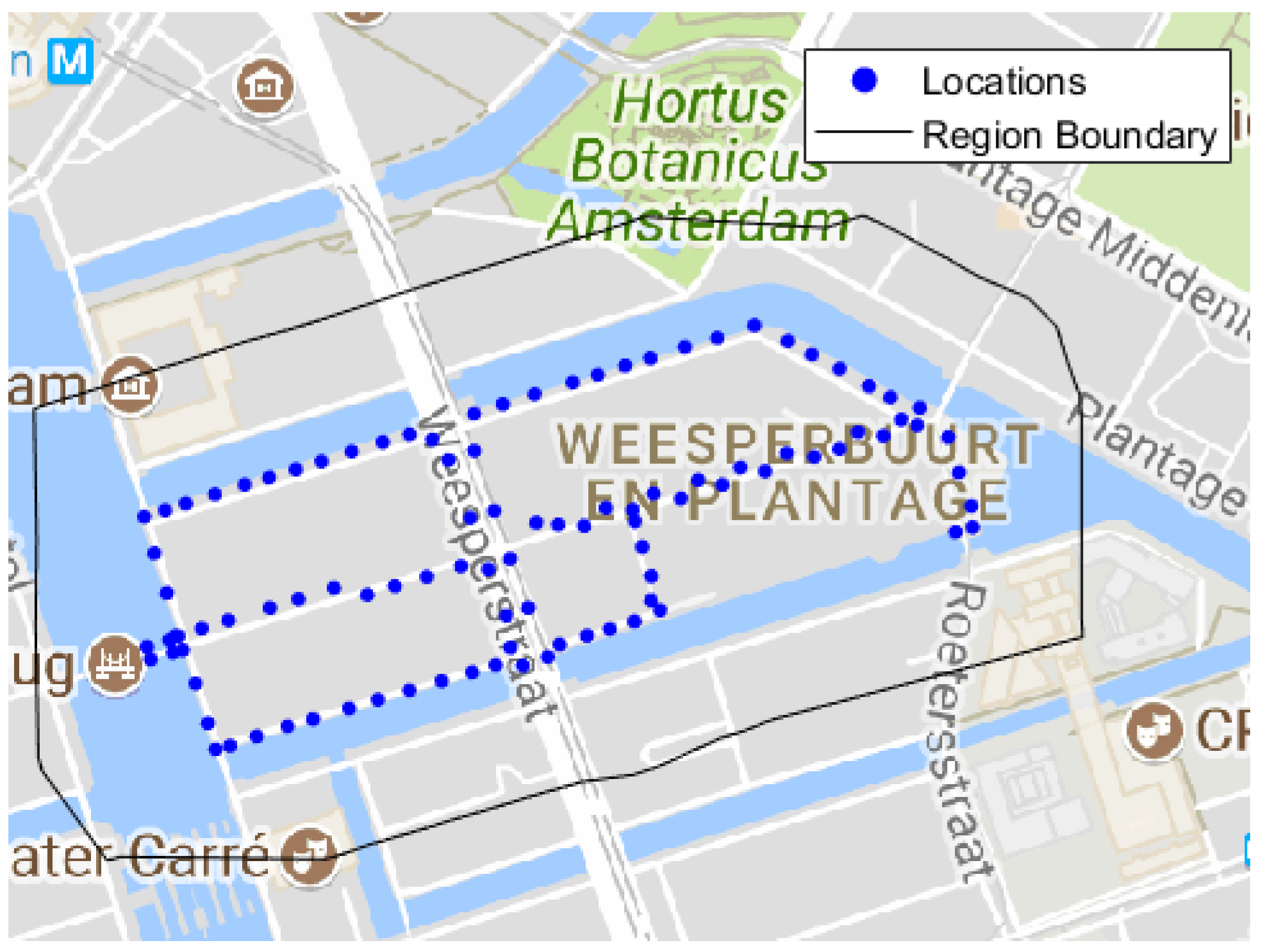
As described in Section 1, the lighting system is used as a set of candidate access locations which can be equipped with services. Data on the locations of lampposts is publicly available for many cities of the Netherlands. It is accessible via Dataplatform, which is an initiative of Civity (Zeist, The Netherlands). The test instances describe various subareas of the city of Amsterdam. The fixed opening costs of a location are taken to be equal to $f_j=5000$ for every location $j\in \mathcal{L}$. A mapping of all locations of some small subarea of the city of Amsterdam can be found in Figure 1.

5.2.2. Services

In total, three services will be considered for the test instances. The various services and their parameter values are based on the works of [35,36]. As previously stated, a service is characterised by its range and its capacity. The capacity is defined as the maximum number of connections it could have at the same time. It is assumed that every service has a circular coverage area. Given the range, the coverage matrix with elements $a_{ij}^u$ can be filled. For every service, information is provided in

Table 2. Overview of the considered services for the test instances.

Service	Range	Capacity ${\mathit{\eta }}_{\mathit{j}}^{\mathit{u}}$	Costs ${\mathit{c}}_{\mathit{j}}^{\mathit{u}}$
$u=1$: WiFi	100	30 $\forall j\in \mathcal{L}$	300 $\forall j\in \mathcal{L}$
$u=2$: SVC	200	15 $\forall j\in \mathcal{L}$	350 $\forall j\in \mathcal{L}$
$u=3$: Alarm	300	∞$\forall j\in \mathcal{L}$	150 $\forall j\in \mathcal{L}$

on the range, capacity, and opening costs of the service. The first service is a WiFi service. It has a range of 100 m, can serve up to a maximum of 30 demand points, and its opening cost is equal to 300. The second service is a Smart Vehicle Communication (SVC) service, which aims at providing data to drivers. It has a range of 200 m, a capacity of 15 connections, and an opening cost of 300. The last service is an Alarm service, which has an unlimited capacity. This service has a range of 300 m, and opening cost equal to 150. The Alarm service aims at providing a loud signal to warn humans about dangers. As the service provision is independent from the number of humans within the range of the access location, the capacity of the service is unlimited.

5.2.3. Demand Points

Every demand point requires service for only one service, and in turn every service has its own disjoint set of demand points. Although sets of demand points differ across the various test instances, every set is generated by the same procedure. The demand points are generated within the boundary that specifies the test area. An example of all demand points classified per service in some small subarea of the city of Amsterdam is given in Figure 2.

For the WiFi service, the home addresses located inside the boundary are taken as demand points. All houses are assigned a demand of one. As the second service is an SVC technique, which aims at providing data to drivers, the demand points are generated on the roads inside the boundary. In contrast to the WiFi service, not every road point has a demand of one. In fact, a demand point is assigned a demand 1, 2, or 3, depending on its characteristics. Demand points referring to so called “A-roads” are assigned a demand of 3, simulating the fact that these important highways are in general congested. These roads are labelled as motorways, and freeways in the original documentation (OpenStreetMap). Less important roads are national and regional roads. These roads are labelled primary and secondary roads, and a demand of 2 is assigned to demand points on such roads. All other roads are of least importance, and in turn are assigned a demand equal to one.

The last service is the Alarm service. As it has an infinite capacity, serving its demand points can be approached as a covering problem instead of some capacitated supply problem. In line with this approach, the demand points of the alarm are intersections of a grid. It is indicated in [37] that this approach works best with regard to computational efficiency. For more information on the generation of the grid, we refer to Section 6.3 of [35]. Similar to the WiFi service, a demand of one is assigned to every demand point. However, the optimal solution is the same for other demand values, as the Alarm service has an unlimited capacity. Hence, for efficiency reasons, a demand of one is assigned.

Note that the demand points that are not located in range of at least one location are excluded from the set of demand points. That is, when there is no location in the neighbourhood of a demand point, it is deleted from the set of demand points.

5.3. Test Instances

The MSCFLP will be solved on a number of test instances, as shown in

Table 3. Overview of the test instances.

Inst.	No. Locations	No. Demand points			Tot.
	$\left|\mathcal{L}\right|$	$|{\mathcal{G}}^1|$	$|{\mathcal{G}}^2|$	$|{\mathcal{G}}^3|$	$\left|\mathcal{G}\right|$
1	33	47	3	9	59
2	77	73	8	15	96
3	99	260	9	13	282
4	102	462	8	15	485
5	400	111	20	25	156
6 ${}^1$	782	21	93	104	218
7	516	1241	42	46	1329
8	6079	8106	397	326	8829
9 ${}^1$	6981	10,122	528	431	11,081

${}^1$ For these two test instances, some demand points requiring WiFi or SVC service are excluded from the initial set of demand points, as these demand points could not be served from any location. Per service, at most five demand points were deleted.

. These test instances are small subareas of the city of Amsterdam. In total, nine test instances are considered, of which instances 1 to 7 are the small instances.

6. Computational Results

In this section, the computational results will be discussed. In [3], the impact of the capacity constraints on the calculation time was shown and stopping criteria are defined. Here, first an analysis is done on the order of the services within the Ordered Sequential Solving Heuristic. Next, the performance of the two solution approaches is compared to the exact approach.

6.1. Order Selection of the Ordered Sequential Solving Heuristic with Updating

In Section 4.2, we already stated that the order in which the various services is considered is important, as it affects the overall solution (quality). For this reason, an analysis is conducted on the six permutations of the set of services to determine the selection order. The OSSHU is applied to all instances for every order with a maximum running time of 1800 s (i.e., 0.5 h) per step. In

Table 4. Results generated by using the OSSHU with a maximum running time of 1800 s per step. Column 2 shows the objective value of the best solution and columns 3–8 show the cost differences with respect to this minimum.

Inst.	Best obj.	Cost Differences (%) c.t. the Best Solution
3-2-1	3-1-2	2-3-1	2-1-3	1-3-2	1-2-3
1	11,100	45.0	45.0	45.0	45.0	0.0	0.0
2	21,700	0.0	1.6	0.0	0.0	1.6	1.6
3	48,200	0.0	0.0	0.0	0.0	0.0	0.0
4	85,650	0.0	0.0	0.2	0.0	0.0	0.0
5	43,150	23.2 ${}^1$	23.2 ${}^1$	11.6 ${}^1$	11.6 ${}^1$	0.0	0.0
6	109,700	13.9	18.5	0.0	0.0	14.2	0.6
7	230,600	0.0	0.2	0.1	0.0	0.2	0.2
8	1,882,550	1.4 ${}^1$	0.6 ${}^1$	3.2 ${}^1$	2.5 ${}^1$	0.3 ${}^1$	0.0 ${}^1$
9	2,351,150	3.4 ${}^1$	1.9 ${}^1$	0.3 ${}^1$	0.7 ${}^1$	0.2 ${}^1$	0.0 ${}^1$

${}^1$ One or multiple steps of the heuristic are terminated, since the maximum running time was reached.

, information is provided on the objective value of the best solution of all permutations. Furthermore, for every order and every instance, information is provided on the relative cost differences compared to the best solution: the higher the relative cost differences, the worse the solution generated by the order. Just as before, the WiFi service is denoted by 1, the SVC service by 2, and the Alarm service by 3.

Table 4 shows that orders 1–4 yield unsatisfactory solutions, especially for instance 1. This is due to the fact that instance 1 is small in size, which implies that only one service access point for the SVC and Alarm service is sufficient to serve all corresponding demand points. If during the first step of the heuristic approach either the SVC or Alarm service access point is selected inefficiently, an additional location needs to be opened in one of the subsequent steps, which yields a relatively large cost difference with respect to the best solution. In instances 2 and 3, it also suffices to have only one service point for the SVC and Alarm services to serve all demand points. However, for these two instances, the first four orders do yield good solutions. This result is explained by the fact that these instances span a slightly larger surface, which implies that both the SVC and the Alarm service access point need to be opened at one of the central locations. Since some of the WiFi demand points are also located in the centre of the area, the Alarm and SVC service access points are easily combined with a WiFi service access point. Observing all instances, we can conclude that mainly the first element of the order determines whether the order yields bad solutions, and, if so, how bad the solutions will be. As an example, the two orders that consider the Alarm service first (i.e., orders 1 and 2) yield the worst solutions for instance 5 compared to the other orders. Similarly, the two orders that consider the WiFi service first yield the best solution for instance 5. These two orders give good solutions not only for instance 5. In general, the last order results in the best solution. Summarising, based on this small analysis, the last order 1-2-3 (i.e., WiFi-SVC-Alarm) is selected for the OSSHU.

Besides this data driven approach to determine the order, we could also look at the various service specifications. The WiFi service has the smallest range and needs to serve the most demand points (relative to its capacity) in general. Contrary to the WiFi service, the Alarm service has a large range, unlimited capacity, and only needs to service a relatively small number of demand points. Thus, the various specifications of the WiFi service will most likely have a larger effect on the location assignment than the specifications of the Alarm service. Therefore, the order WiFi-SVC-Alarm seems to be appropriate.

6.2. Performance

In this section, we will present the performance of the two heuristic approaches of Chapter 4, together with the performance of an exact approach. For the exact approach, CPLEX is used to solve the ILP to optimise the location assignments of the various services simultaneously. The results of both heuristics and the exact approach are presented in

Table 5. Objective values and corresponding running times for the SSH (columns 2 and 3), for the OSSHU (columns 4 and 5), and for the exact method (columns 6–8). Columns 9–11 show the relative cost differences between the various solution approaches.

	SSH		OSSHU		Exact Method			Cost differences (%)
	Obj.	Time (s)	Obj.	Time (s)	Obj.	Gap	Time (s)	SSH-OSSHU	SSH-Exact	OSSHU-Exact
1	16,100	0.1	11,100	0.0	11,100	0.0	1.1	31.1	31.1	0.0
2	31,700	0.2	22,050	0.2	21,700	0.0	22.1	30.4	31.5	1.6
3	63,550	0.6	48,200	0.7	48,200 ${}^1$	3.7	4.9	24.2	24.2	0.0
4	100,650	0.8	85,650	0.9	85,650 ${}^1$	4.0	6.4	14.9	14.9	0.0
5	58,150	1.4	43,150	3.6	38,150 ${}^1$	9.9	43,200.0	25.8	34.4	11.6
6	164,250	118.9	110,400	2.6	100,200	0.0	171.8	32.8	39.0	9.2
7	270,600	984.5	230,950	1,029.8	231,600 ${}^1$	2.5	316.6	14.7	14.4	−0.3
8	2,007,950 ${}^1$	129,600.0	1,704,800	28,867.4	1,718,450 ${}^1$	7.6	43,200.0	15.1	14.4	−0.8
9	2,494,950 ${}^1$	129,600.0	2,462,350	29,319.5	2,192,800 ${}^1$	9.8	43,200.0	1.3	12.1	10.9

${}^1$ This approach is terminated or some steps of this approach are terminated according to the stopping criteria of [3]. The maximum running time per step of the SSH is 43,200 s (i.e., 12 h) and the maximum running time per step of the OSSHU is 14,400 s (i.e., 4 h).

. The table provides information on the objective value, the running times, and the cost differences of the various approaches. Firstly, we assess the performance of the SSH relative to the exact approach. Secondly, we discuss the performance of the OSSHU relative to the SSH and the exact approach.

6.2.1. Sequential Solving Heuristic versus Exact Method

In the SSH, the location assignments of the services are optimised one by one, and the solutions of the various steps are combined to get a multi-service location assignment. Contrary to the SSH, the exact method optimises these location assignments simultaneously. By comparing both approaches, we are able to get some insights into the added value of simultaneous optimisation of the location assignments compared to one by one optimisation. The exact method is expected to provide better solutions than the SSH, but the SSH is expected to yield lower overall running times. In [3], it was shown that the running time of the solver increases tremendously with the problem size even for non-binding capacity limits. Thus, the SSH seems to be a valuable alternative solution approach. The stopping criteria of [3] is evaluated for each step of this heuristic approach, which implies that the maximum running time of the heuristic is 36 h.

Columns 3 and 8 of Table 5 provide the running times of the SSH and the exact method, respectively. For instances 1–6, the running time of the exact method exceeds the running time of the SSH. In contrast, for instances 7–9, a reverse statement holds. For instances 8 and 9, this result is explained by the fact that all steps of the SSH have been terminated as the maximum running time had been reached. The high running time of the SSH for instance 7 is a consequence of the optimisation of the WiFi service, which took 948.6 s. This is most likely the result of the relatively large number of WiFi demand points compared to the first six instances.

Column 10 of Table 5 shows that there is a large relative cost difference between the heuristic and the exact method for all instances. The total costs of the SSH solution exceed the exact solution on average by $24.0\%$. This, combined with the limited gain on calculation time, implies that simultaneous optimisation is preferred over one by one optimisation, although it yields higher running times in some situations.

6.2.2. Performance of the Ordered Sequential Solving Heuristic with Updating

Again, the exact method is expected to provide better solutions than the OSSHU, but the heuristic is expected to yield lower overall running times. Similarly, relative to the SSH, the OSSHU is expected to find better solutions. Columns 3 and 5 of Table 5 provide the running times of the SSH and the OSSHU, respectively. The running times of the OSSHU are in most cases similar to the running times of the SSH. However, column 9 shows that the OSSHU performs significantly better than the SSH. The total relative cost difference is equal to $21.1\%$ on average. This result shows the importance of intermediate cost updates. The intermediate cost updates ensure that access locations of previously considered services are preferred over locations that are not yet equipped with services, such that cost benefits are obtained. Summarising, the OSSHU outperforms the SSH, while running times are similar to the running times of the SSH.

If we now compare the performance of the OSSHU with the performance of the exact method, several conclusions can be drawn. Except for instance 7, the running times of the OSSHU are shorter than the running times of the exact method. Furthermore, considering instances 1–4, the results in column 11 of Table 5 indicate that the heuristic is able to find similar solutions as the exact method. Contrary to these instances, the heuristic does not find good solutions for instances 5, 6, and 9. This is most likely due to the fact that the WiFi demand points in these instances are located only in a relatively small subarea of the instances. Compared to, for example, instance 7, the distribution of the WiFi demand points is less diffuse over the surface, implying that the heuristic cannot find good solutions for such instances. Moreover, extending the maximum running time from 1800 to 14,400 s per step implies that the heuristic finds a worse solution for instance 9. Table 4 shows that the heuristic finds a solution with total costs of 2,351,150 subject to a maximum running time of 1800 s per step, but Table 5 shows that the heuristic finds a worse solution with total costs equal to 2,462,350 when the maximum running time is 14,400 s per step. The most likely causes of this result are the distribution of the WiFi demand points and the limit on the maximum running time, since a maximum running time of 43,200 s per step does yield a better solution.

However, when we consider instances 7 and 8, a different conclusion is drawn. The experiments show that, for these instances, the OSSHU finds better solutions than the exact method in a shorter running time. Of course, these results are sensitive to the maximum running time, since both approaches are terminated due to this stopping criteria. However, these results show that breaking up the joint optimisation problem into multiple subproblems combined with intermediate cost updates can lower the running time, while decreasing the total costs for larger instances. It is believed that the heuristic finds even better solutions, when the maximum running time of 12 h is divided over the various steps more efficiently.

In summary, we can conclude that, for very small instances, the OSSHU yields (near-)optimal solutions. It provides significantly better solutions than the SSH, showing the importance of intermediate cost updating. However, when WiFi demand points are not well spread across the area, the OSSHU solutions are of poor quality. Nevertheless, on larger instances, the heuristic can outperform the exact method in short running times. This result shows that it is beneficial to break the joint optimisation problem into multiple subproblems and combine this with intermediate cost updates when dealing with large instances.

7. Conclusions

In this paper, we optimised the distribution of multiple services in urban areas. We took the Multi-Service Capacitated Facility Location Problem (MSCFLP). It aims at optimising the distribution of multiple services simultaneously in some urban area, such that the total costs are minimised, while satisfying all demand requirements. For this problem, an integer linear program (ILP) was formulated. Two heuristic approaches were proposed to solve the problem for each service separately and then combine the solutions. One heuristic, however, updated the cost parameters between the successive steps. The last approach yields lower calculation times and still acceptable solutions compared with the solution obtained from solving the ILP to optimality. These results show that breaking up the joint optimisation problem into multiple subproblems combined with intermediate cost updates can lower the running time, while decreasing the total costs for larger instances. This could be a good starting point for a heuristic approach, as we see that the scalability for larger real world problems is still low.

Several opportunities exist for future work in this research area. First, some heuristic approaches can be developed to improve the calculation time for larger problem sizes. Second, one could extend the base model by allowing for multiple services boxes of the same service on one access location. For this extension, next to determining which locations should be equipped with services, it has to be decided how many service boxes should be opened per service on these locations. Third, a partial covering extension could be made, in which not all demand points have to be covered.

References

- Calvillo, C.; Sànchez-Miralles, A.; Villar, J. Energy management and planning in smart cities. Renew. Sustain. Energy Rev. 2016, 55, 273–287. [Google Scholar] [CrossRef]
- Sarkar, S.; Dixit, S.; Mukherjee, B. Hybrid Wireless-Optical Broadband Access Network (WOBAN): Network Planning and Setup. IEEE J. Sel. Areas Commun. 2008, 26, 12–21. [Google Scholar] [CrossRef]
- Hoekstra, G.; Phillipson, F. Location Assignment of Capacitated Services in Smart Cities. In Proceedings of the 4th International Conference on Mobile, Secure and Programmable Networks (MSPN 2018), Paris, France, 18–20 June 2018. [Google Scholar]
- Vos, T.; Phillipson, F. Dense Multi-Service Planning in Smart Cities. In Proceedings of the International Conference on Information Society and Smart Cities, Cambridge, UK, 27–28 June 2018. [Google Scholar]
- Albino, V.; Berardi, U.; Dangelico, R.M. Smart Cities: Definitions, Dimensions, Performance, and Initiatives. J. Urban Technol. 2015, 22, 3–21. [Google Scholar] [CrossRef]
- Georgakopoulos, D.; Jayaraman, P.P. Internet of things: From internet scale sensing to smart services. Computing 2016, 98, 1041–1058. [Google Scholar] [CrossRef]
- Rathore, M.M.; Paul, A.; Ahmad, A.; Chilamkurthi, N.; Hong, W.-W. Real-time secure communication for Smart City in high-speed Big Data environment. Future Gen. Comput. Syst. 2017, 83, 638–652. [Google Scholar] [CrossRef]
- Rathore, M.M.; Ahmad, A.; Paul, A.; Rho, S. Urban planning and buidling smart cities based on the Internet of Things using Big Data analytics. Comput. Netw. 2016, 101, 63–80. [Google Scholar] [CrossRef]
- Peralta, A.; Inga, E.; Hincapié, R. Optimal Scalability of FiWi Networks Based on Multistage Stochastic Programming and Policies. Opt. Soc. Am. 2017, 9, 1172–1183. [Google Scholar]
- Krarup, J.; Pruzan, P. The simple plant location problem: Survey and synthesis. Eur. J. Oper. Res. 1983, 12, 36–81. [Google Scholar] [CrossRef]
- Akinc, U.; Khumawala, B. An efficient branch and bound heuristic for the capacitated warehoues location problem. Manag. Sci. 1977, 23, 585–594. [Google Scholar] [CrossRef]
- Klose, A.; Görtz, S. A branc-and-price alorithm for the capacitated facility location problem. Eur. J. Oper. Res. 2007, 179, 1109–1125. [Google Scholar] [CrossRef]
- Wentges, P. Accelerating Benders’ decomposition for the capacitated facility location problem. Math. Methods Oper. Res. 1996, 44, 267–290. [Google Scholar] [CrossRef]
- Kuehn, A.; Hambuger, B. A heuristic program for locating warehouses. Manag. Sci. 1963, 9, 643–666. [Google Scholar] [CrossRef]
- Feldman, E.; Lehrer, F.; Ray, T. Warehouse location under continuous economies of scale. Manag. Sci. 1966, 12, 670–684. [Google Scholar] [CrossRef]
- Jacobsen, S. Heuristics for the capacitated plant location model. Eur. J. Oper. Res. 1983, 12, 253–261. [Google Scholar] [CrossRef]
- Mahdian, M.; Ye, Y.; Zhang, J. Approximation algorithms for metric facility location problems. SIAM J. Comput. 2003, 36, 411–432. [Google Scholar] [CrossRef]
- Sridharan, R. The capacitated plant location problem. Eur. J. Oper. Res. 1995, 87, 203–213. [Google Scholar] [CrossRef]
- Magnanti, T.; Wong, R. Decomposition methods for facility location problems. In Discrete Location Theory; Mirchandani, P., Francis, R., Eds.; John Wiley and Sons, Inc.: New York, NY, USA, 1990; pp. 209–262. [Google Scholar]
- Fisk, J. A solution procedure for a special type of capacitated warehouse location problem. Logist. Transp. Rev. 1978, 13, 305–320. [Google Scholar]
- Barcelo, J.; Casanovas, J. A heuristic Lagrangian algorithm for the capacitated plant location problem. Eur. J. Oper. Res. 1984, 15, 212–226. [Google Scholar] [CrossRef]
- Klincewicz, J.; Luss, H. A Lagrangian relaxation heuristic for capacitated facility location with single source constraints. J. Oper. Res. Soc. 1986, 37, 495–500. [Google Scholar] [CrossRef]
- Pirkul, H. Efficient algorithm for the capacitated concentrator location problem. Comput. Oper. Res. 1987, 14, 197–208. [Google Scholar] [CrossRef]
- Guastaroba, G.; Speranza, M. A heuristic for BILP problems: The Single Source Capacitated Facility Location Problem. Eur. J. Oper. Res. 2014, 238, 438–450. [Google Scholar] [CrossRef]
- Rönnqvist, M.; Tragantalerngsak, S.; Holt, J. A repeated matching heuristic for the single-source capacitated facility location problem. Eur. J. Oper. Res. 1999, 116, 51–68. [Google Scholar] [CrossRef]
- Warszawski, A. Multi-dimensional location problems. Oper. Res. Q. 1973, 24, 165–179. [Google Scholar] [CrossRef]
- Warszawski, A.; Peer, S. Optimizing the location of facilities on a building site. Oper. Res. Q. 1973, 24, 35–44. [Google Scholar] [CrossRef]
- Geoffrion, A.; Graves, G. Mutlicommodity distribution system design by Benders decomposition. Manag. Sci. 1974, 20, 822–844. [Google Scholar] [CrossRef]
- Pirkul, H.; Jayaraman, V. A multi-commodity, multi-plant, capacitated facility location problem: Formulation and efficient heuristic solution. Manag. Sci. 1998, 25, 869–878. [Google Scholar] [CrossRef]
- Hinojosa, Y.; Puerto, J.; Fernández, F. A mltiperiod two-echelon multicommodity capacitated plant location problem. Eur. J. Oper. Res. 2000, 123, 271–291. [Google Scholar] [CrossRef]
- Canel, C.; Khumawala, B.; Law, J.; Loh, A. An algorithm for the capacitated, multi-commodity, multi-period facility location problem. Comput. Oper. Res. 2001, 28, 411–427. [Google Scholar] [CrossRef]
- Melo, M.; Nickel, S.; Saldanha da Gama, F. Dynamic multi-commodity capacitated facility location: A mathematical modeling framework for strategic supply chain planning. Comput. Oper. Res. 2005, 33, 181–208. [Google Scholar] [CrossRef]
- Li, J.; Chu, F.; Prins, C. Lower and upper bounds for a capacitated plant location problem with multicommodity flow. Comput. Oper. Res. 2009, 36, 3019–3030. [Google Scholar] [CrossRef]
- Li, J.; Chu, F.; Prins, C.; Zhu, Z. Lower and upper bounds for a two-stage capacitated facility location problem with handling costs. Eur. J. Oper. Res. 2014, 236, 957–967. [Google Scholar] [CrossRef]
- Vos, T. Using Lamppost to Provide Urban Areas With Multiple Services. Master’s Thesis, Erasmus University Rotterdam and TNO, Rotterdam, The Netherlands, 20 August 2016. [Google Scholar]
- Verhoek, M. Optimising the Placement of Access Points for Smart City Services with Stochastic Demand. Master’s Thesis, University of Groningen and TNO, Groningen, The Netherlands, 26 July 2017. [Google Scholar]
- Murray, A.T.; O’Kelly, M.E.; Church, R.L. Regional service coverage modelling. Comput. Oper. Res. 2008, 35, 339–355. [Google Scholar] [CrossRef]
Figure 1.
Mapping of all access locations in some small subareas of the city of Amsterdam.
Figure 2.
Plot of the demand points per service of some small area in Amsterdam.