Revenue Implications of Strategic and External Auction Risk

Abstract

Two experimental treatments are used to study the effects of auction risk across five mechanisms. The first canonical, baseline treatment features only strategic risk and replicates the standard results that overbidding relative to the risk neutral Nash equilibrium is prevalent in all common auction mechanisms except for the English auction. We do not find evidence that bidders’ measured risk preferences can explain these patterns of overbidding. To enhance salience, we introduce a second novel treatment with external risk. This treatment captures the risk, prevalent in online auctions, that winners will not receive a good of value. We find that dynamic auctions—including the English—are particularly susceptible to overbidding in this environment. We note that overbidding is somewhat diminished in later periods and that our results may thus have particular relevance for bidders who are not highly experienced or who have not directly experienced losses. We conclude with a brief discussion of research implications.

1. Introduction

Bidders in the field must confront two sorts of risk. The first, and the principal focus of most economic studies, is strategic risk. Bidders who weigh how much to “shade their bids” in a first-price sealed bid auction, for example, are engaged in strategic risk management. The second, which has drawn less attention from economists in private value auctions, is external risk. The prospect that, when all is said and done, the prize over which bidders compete proves to be defective is an example of external risk.

This second sort of risk has particular practical importance given the prevalence of online auctions, in which bidders are often unable to inspect goods prior to the auction or even ensure receipt after winning [1,2]. Auction fraud, defined as the misrepresentation of or the failure to deliver goods, is among the top two internet crimes reported in the United States each year [3].1 Even in the absence of intentional seller deception, there is external risk for bidders who must accept goods “as is”, without prior inspection, a common requirement of auctions for surplus or impounded items. It is therefore surprising that the empirical literature on the response to such risk, or on differences in “risk pricing” across mechanisms, is thin. While some researchers have found that seller reputation ratings, particularly negative ratings, have a small but significant influence on prices [4,5,6], it has proven difficult, in the absence of data on bidders’ values and beliefs, to determine whether adjusted prices reflect actual risk. Furthermore, because almost all of these studies concern online variants of the English auction, mechanism-specific effects are never considered.

Induced value lab experiments offer an important platform from which to explore these questions, as bidder values, receipt risk, and mechanism can all be controlled. There is now a large literature that compares auction revenue across formats in induced independent private value auctions. One of the most robust findings in this literature is the presence of “overbidding” [7,8] relative to the risk neutral Nash equilibrium (RNNE) under the first-price, Dutch, and all-pay mechanisms. With some important exceptions [9,10], overbidding is also not uncommon in second-price auctions. A common, but much debated, explanation for overbidding in the first two formats centers on risk preferences: risk averse bidders in both the first-price and Dutch auctions should be willing to trade off the size of the surplus, conditional on winning, against an increase in the likelihood of winning. Direct tests of whether overbidding in first-price and Dutch auctions is correlated with an individual’s risk aversion in other contexts is limited. In one such test, [11] find that estimates of risk aversion derived from first-price sealed bid auctions are negatively correlated with estimates derived from a Becker-DeGroot-Marschak task.2 Other common explanations for overbidding in the Dutch and first-price auctions include anticipated regret, if an auction loser eventually learns that the good sold at a price less than her value [15], and biased probabilistic beliefs, such that individuals systematically underestimate their probability of winning conditional on their value [16]. Across formats, overbidding can also be attributed to participants receiving extra utility from the “joy of winning” the auction [17] or competitive arousal activated by time pressure and rivalry [18].

In contrast to the overbidding observed in other formats, participants in induced private value English auctions tend to bid just up to their values, consistent with the RNNE prediction [7]. There is some evidence, however, that outside the induced values context, English auction bidders can be mistake-prone: [19], for example, find that higher shipping costs are not priced into bids, while [20] conclude that bidders in dynamic auctions often bid above their stated maximum willingness to pay. These studies suggest that English auction bidders might not necessarily be as successful in environments where their value for the good is not given by an explicitly assigned, certain payoff. Auctions with external risk offer the opportunity to test in a controlled environment whether English auction bidders are also susceptible to overbidding outside of a riskless induced value setting and whether the simple introduction of a well-defined probability that the good will not be delivered is sufficient to trigger such behavior.

To better understand the overbidding phenomenon in a salient and practical environment, we introduce a much simplified form of external risk: namely, a fixed likelihood that the winner will never receive the value of the item. In particular, we use an induced independent private values lab experiment to study revenues under five common mechanisms—first-price sealed bid (FP), second-price sealed bid (SP), English (E), Dutch (D), and all-pay (AP)—and two risk conditions, one in which the winner receives her private value with certainty, and another in which there is a 20% likelihood that the winner receives nothing at all. The advantage of this approach is that we are able to control bidder beliefs about the likelihood of loss. In the absence of concerns about misperceived risk, betrayal aversion, or other social preferences, we obtain cleaner measures of bidder response under each mechanism. In contrast to standard independent private value auctions, the introduction of this second risk in auctions with risk averse bidders should suppress overbidding relative to the RNNE prediction, with underbidding expected in both the English and SP. If, however, consistent with [19], bidders fail to price the “terms of sale” into the bids or, following [20], revise WTP upward during auctions, we should observe more overbidding, especially in the English auction.

Our main contribution is the introduction of a form of external risk—one consistent with the existence of, say, seller fraud or uncertainty about product quality—into the five canonical private value auctions. We are agnostic about the interpretation of the external risk, but the possibilities include stylized representations of seller fraud, or the purchase of counterfeit or defective goods, or the acquisition of goods that, through no fault of the seller, otherwise prove to be valueless. We are unaware of any other experimental work on this important question, but note that other manifestations of risk have been investigated. In particular, there is a large literature on common value auctions, in which bidders receive independent signals about the common value. Participants tend to systematically overbid in these auctions, as they fail to correct for the “winner’s curse” by taking into account the fact that the winner likely received an extreme signal. Such work has found that participants are less susceptible to the winner’s curse in the English auction, where bidders can update their beliefs as they observe competitors dropping out, than in the first-price sealed bid auction, where they cannot [8]. A pair of studies investigate ambiguity aversion by studying whether different prices will arise in markets for an asset that pays a random dividend with known versus unknown probability: [21] find that the market price for the ambiguous asset is lower than for the risky asset, regardless of whether the allocation is determined by a first-price sealed bid auction or a double-auction market, while [22] allow participants to choose which auction they wish to bid in, finding that the most risk tolerant individuals bid on the ambiguous asset and market prices are equal. While suggestive of the possibility that participants may be able to price risk into auctions, and that it may differ across formats, this work does not allow us to generalize to overbidding in risky, private value auctions. The authors of [23] conduct a private value auction in which participants know only an interval in which their value falls, rather than the precise value, to model the imprecision with which individuals perceive willingness to pay. They find that revenue is very close to the risk neutral equilibrium predictions in both proxy and standard ascending auctions but that “auction fever” can be induced by informing participants that they are the current high bidder. They suggest that bidders who start to see themselves as the eventual winner may increase their willingness to pay over the course the auction, similarly to the findings of [20], as the result of a pseudo-endowment effect. This study provides further evidence that English auction bidders who are not assigned precise induced values may also be prone to overbidding in some contexts.

We find that, as expected, revenues under all mechanisms decline with the introduction of external risk. However, the revenues of risky auctions exceed the adjusted RNNE prediction in just the two “real time” mechanisms—that is, the English and the Dutch—and the AP. In other words, the English auction, which reliably produces predicted revenues in riskless induced value lab experiments, becomes particularly susceptible to overbidding when winners face the risk of not receiving the good that they have purchased. These results suggest that bidders in dynamic auctions may have particular difficulty adjusting their bids to account for the type of risks common in online auctions—even in a simple environment where there is no uncertainty about the risks that they face. To further investigate whether bidder learning could influence behavior, we separate our data into early periods and later periods. We find that higher than expected revenues persist throughout the experiment, but that the revenues in the dynamic risky auctions are highest at the beginning of the experiment, suggesting that, with enough experience, bidders may eventually bid closer to the risk neutral prediction.

In addition to these results, we report several other findings. First, in the absence of external risk, and consistent with previous experimental results, we find that most participants overbid relative to the RNNE prediction in all but the English auction and that, as a result, revenues in all auctions but the English are greater than predicted. Second, we find direct evidence for the proposition that the all-pay auction generates more revenue than the FP, or any other winner-pay auction, in practice. Third, we directly measure risk aversion of each bidder using both an externally-validated survey question and an incentivized lottery choice. However, we find no evidence that risk aversion is positively correlated with overbidding or revenues under any mechanism. Because we are not aware of a similar direct test of whether elicited risk preferences predict overbidding under different mechanisms, we consider this another important contribution to the literature, but note that our findings are in line with [11]’s comparison of behavior in first-price auctions and in a Becker-DeGroot-Marschak procedure. We are therefore able to replicate some common results and to provide new evidence against one popular explanation for these results.

2. Background and Predictions

In the canonical case with risk neutral bidders, whose independent and private values are drawn from some common distribution, the theoretical implications of external risk are straightforward. In each mechanism, the winner now receives, in expectation, $(1-\theta )v_i$, where θ is the likelihood that the buyer never receives the value of the good, and $v_i$ is her private value. In effect, the external risk is the equivalent of an ad valorem tax on the value of the prize to the winner. It follows that in the symmetric equilibrium for each mechanism, bids and therefore expected revenue are scaled down θ percent, so that revenue equivalence is preserved. There is no need to (re)derive these well-known bid functions here. Instead, we note that in the special case of interest here, in which the private values of four bidders are drawn from a uniform $[0,100]$ distribution, FP bidders should submit, and D bidders should stop the auction when, ${\sigma }^{FP}\left(v\right)={\sigma }^D\left(v\right)=0.75(1-\theta )v$; SP bidders should submit, and E auction bidders should drop out when, ${\sigma }^{SP}\left(v\right)={\sigma }^E\left(v\right)=(1-\theta )v$; and AP bidders should submit ${\sigma }^{AP}=(7.5\times {10}^{-7})(1-\theta )v^4$. Under all five mechanisms, expected revenue is therefore equal to $60(1-\theta )$. For the two cases considered here, $\theta =0$ and $\theta =0.2$, the introduction of external risk should cause mean revenues to fall, from 60 to 48.

When $\theta =0$, risk averse bidders will bid above the RNNE prediction in FP and D, but not in SP or E. It follows that risk averse expected revenues are 60 in SP and E but more than 60 in FP and D. Expected revenues in AP auctions with risk averse bidders can be higher or lower than the RNNE [24]. When $\theta =0.2$, however, risk preferences should matter even in SP and E auctions: in particular, risk averse bidders should underbid relative to the RNNE prediction, and submit a bid equal to the certainty equivalent in a $[0.8,v_i;0.2,0]$ lottery. In the D and FP, the presence of risk averse bidders should generate less overbidding relative to the case of $\theta =0$, with underbidding possible. The intuition here is straightforward: risk aversion causes participants in the FP and D auctions to bid a higher fraction of their value from winning. In the presence of external risk, however, risk aversion simultaneously decreases the value of winning the auction, with a net effect that can be underbidding or slight overbidding, as illustrated below.

To provide a simple but illustrative example of the effects of risk aversion, suppose that all bidders have the CRRA utility function $u\left(x\right)=x^{\alpha }$. In the absence of external risk, it is not difficult to show that the equilibrium bid functions under the FP and D mechanisms are now:

$${\sigma }^{FP}\left(v\right)={\sigma }^D\left(v\right)=\left[\frac{3}{3+\alpha }\right]v$$

where, as the risk aversion parameter α decreases from 1, bids become more “aggressive” [17]. Since it remains dominant to bid one’s value in the second price and English, we also have ${\sigma }^{SP}\left(v\right)={\sigma }^E\left(v\right)=v$. (We ignore for a moment the case of the AP mechanism, due to the difficulties in providing closed-form solutions under risk aversion [24].) It follows that expected revenues will be:

$$E{R}^{FP}=E{R}^D=\frac{240}{3+\alpha }>60=E{R}^{SP}=E{R}^E$$

when bidders are risk averse ($\alpha <1$).

If we treat the external risk in our design as akin to winning bidders receiving the certainty equivalent of their private values, or in this case $0.8^{\frac{1}{\alpha }}v$, it follows that:

$${\sigma }^{FP}\left(v\right)={\sigma }^D\left(v\right)=\left[\frac{3{(0.8)}^{\frac{1}{\alpha }}}{3+\alpha }\right]v>{(0.8)}^{\frac{1}{\alpha }}v={\sigma }^{SP}\left(v\right)={\sigma }^E\left(v\right)$$

and therefore:

$$E{R}^{FP}=E{R}^D=\frac{240{\left(0.8\right)}^{\frac{1}{\alpha }}}{3+\alpha }>60{\left(0.8\right)}^{\frac{1}{\alpha }}=E{R}^{SP}=E{R}^E$$

when $\alpha <1$. What does this mean in practice? We know that with risk neutral bidders, revenues should fall from 60 (under all mechanisms) to 48 with the introduction of external risk. In the case where $\alpha =0.9,$ for example, expected revenues in the FP and D auctions are above the RNNE predictions before (61.5) and after (48.02) the introduction of external risk, a reduction of $13.48$.3 In the SP and E auctions, expected revenues are equal to the RNNE level (60) in the absence of external risk, and 46.8, which is less than the RNNE, with it, a difference of $13.2$.

3. Experimental Design

The experiment took place at Middlebury College in April 2014. Ten sessions were conducted and 148 students participated in total. Each session consisted of 15 auction periods, with the auction mechanism held constant for the session. The auctions were computerized using the software z-Tree [25]. At the start of each period, participants were randomly matched into groups of four bidders and each participant was assigned a value for the item being auctioned. The values were in experimental dollars and were randomly drawn from a uniform distribution on the [0,100] interval.

In the sealed bid sessions (FP, SP, AP), participants each typed a bid, up to one decimal point. The highest bidder won the item and he was required to pay either his own bid (FP) or the bid of the second highest bidder (SP). In the AP sessions, all participants paid their own bids, regardless of whether they won. In the E sessions, a clock ticked upwards from 0 to 100 experimental dollars, in 10 cent increments. Participants could exit the auction at anytime. The last remaining bidder in the auction won the item and paid the price at which the second to last bidder exited. Finally, in the D sessions, a clock ticked downwards from 100 to 0 experimental dollars, in 10 cent increments. The first player to hit a “Buy Now” button won the auction and paid the price displayed when the button was pressed.

External risk was introduced in the form of a fixed likelihood that the winning bidder would receive the item. Upon learning their values at the start of the period, participants also learned whether the winner would receive his value with probability 1, in which case the auction period was “safe” (S), or with probability 0.8, in which case it was “risky” (R). One could interpret this as the experience of learning about the item and the seller’s rating or reputation at the same time, although other interpretations are possible: e.g., a memorabilia collector may view an online auction while inferring the likelihood that the good will be of value from the posted photographs, or an art collector will sometimes learn that a painting has become available at the same time as doubts about its provenance are revealed. Eight of fifteen auction periods were R periods. Which periods were S vs. R, as well as which R periods resulted in an actual loss, was determined randomly before the experiment and then fixed across all auction groups and sessions to ensure that bidder experience was the same across treatments.

Winners who did not receive the item were still required to pay the relevant price (as were losers in the all-pay auction). After each auction period, bidders learned the price paid and whether the item was received. All bidders received an endowment of 100 experimental dollars, ensuring that a participant who bid the maximum value and sustained a loss would not finish the experiment with negative earnings. To incentivize subjects to treat each auction separately and ensure that the risk was salient across all periods, participants were compensated using the random decision selection mechanism [26]: At the end of the experiment, one period was selected randomly and participants were paid their profits from this period only, at the exchange rate of 15 experimental dollars = 1 US dollar.

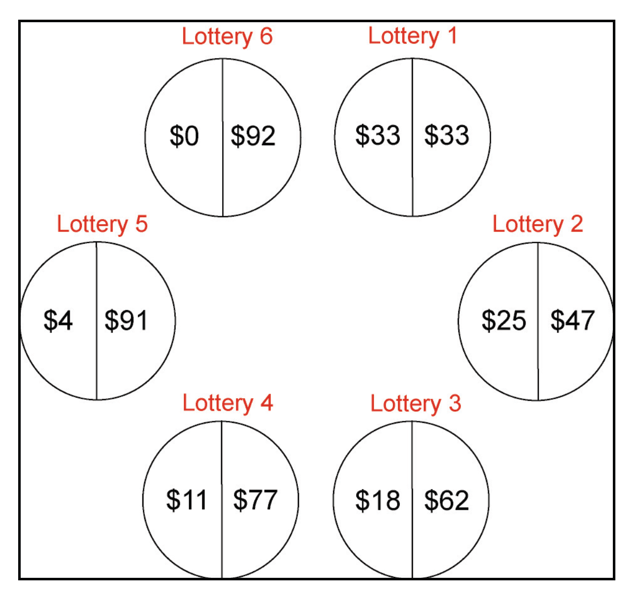
All participants completed a survey approximately one week before participating, which asked demographic questions about their class year, major, and gender, as well as about risk preferences and included an incentivized choice among six lotteries. The lottery choice was taken from a large-scale field experiment [27], and is similar to the elicitation developed by [28], which has been widely adopted in the experimental literature [29]. Participants were shown the six lotteries in Figure 1 and asked to choose one. Each lottery was described as a bag containing five high value balls and five low value balls. They were told that one ball would be drawn from their selected bag and they would be paid the value of that ball, in experimental dollars, at their experimental session. The lotteries were conducted after the main experiment, so that the outcome could not influence their behavior, and the lottery choice was made well in advance of coming to the lab to participate, to minimize the possibility that a desire to be consistent would influence or prime their bidding behavior. Turning to the specific values in Figure 1, Lottery 5 has the highest expected value and thus participants who are risk neutral or close to risk neutral are expected to choose Lottery 5. Lottery 6 has a lower expected value and higher variance, and thus should be chosen only by risk-seeking participants (8.2% of our sample, in line with previous work). Among Lotteries 1 through 4, lower numbers indicate greater risk aversion. In addition, participants responded to a survey question asking, in general, how willing they were to take risks, reported on a 5-point Likert scale. Similar questions are often used in surveys and have been found to be a reliable predictor both of decisions in real-stakes Holt-Laury lottery choices as well as of risky behavior outside the lab, such as smoking, stock market participation, and choosing self-employment [30].

Figure 1. Lottery choice given to participants the week before the experiment.

Figure 1. Lottery choice given to participants the week before the experiment.

4. Results

Our central question is whether RNNE revenues obtain—and, if not, the nature of the deviation—with and without the presence of external risk. The first four columns of Table 1 report, in the form of regression coefficients, mean revenues for each format, with stars indicating whether the revenue differs from the theoretical predictions in S (60) and R (48) auctions. (For expositional purposes, we choose, following [31], to include the full set of indicators and no constant.)

Table 1. Revenue (Models 1–4) and Percent Excess Revenue (Models 5–10) with Average Risk Aversion Controls.

	(1)	(2)	(3)	(4)	(5)	(6)	(7)	(8)	(9)	(10)
	Safe	Safe	Risky	Risky	Safe	Safe	Risky	Risky	Safe	Risky
Dutch	69.16${}^{***}$	69.32${}^{***}$	58.82${}^{***}$	58.80${}^{***}$	0.125${}^{***}$	0.126${}^{***}$	0.201${}^{***}$	0.202${}^{***}$	0.126${}^{***}$	0.202${}^{***}$
	(2.214)	(2.209)	(1.928)	(1.939)	(0.0203)	(0.0204)	(0.0316)	(0.0313)	(0.0258)	(0.0446)
English	60.69	60.46	53.05${}^{**}$	52.83${}^{**}$	–0.00227	–0.00484	0.199${}^{***}$	0.200${}^{***}$	–0.00484	0.200${}^{***}$
	(3.026)	(3.031)	(2.545)	(2.437)	(0.0221)	(0.0225)	(0.0711)	(0.0731)	(0.0351)	(0.00765)
FP	65.20${}^{**}$	65.66${}^{**}$	51.91	51.93${}^{*}$	0.0953${}^{***}$	0.101${}^{***}$	0.0664	0.0699${}^{*}$	0.101${}^{*}$	0.0699${}^{***}$
	(2.512)	(2.513)	(2.380)	(2.378)	(0.0357)	(0.0376)	(0.0418)	(0.0411)	(0.0469)	(0.00199)
SP	65.51${}^{*}$	66.66${}^{*}$	47.31	47.89	0.0390	0.0124	0.0239	0.0151	0.0124	0.0151
	(3.298)	(3.714)	(3.118)	(3.721)	(0.0296)	(0.0280)	(0.0403)	(0.0549)	(0.0141)	(0.0539)
AP	123.2${}^{***}$	123.0${}^{***}$	82.42${}^{***}$	81.46${}^{***}$	1.864${}^{***}$	1.815${}^{***}$	2.114${}^{***}$	2.054${}^{***}$	1.815${}^{***}$	2.054${}^{**}$
	(9.665)	(9.834)	(7.059)	(6.903)	(0.341)	(0.330)	(0.468)	(0.465)	(0.160)	(0.633)
FP × Risk Aversion		–7.653		–0.391		–0.0969		–0.0573	–0.0969${}^{***}$	–0.0573${}^{**}$
		(5.382)		(5.245)		(0.0692)		(0.0970)	(0.0211)	(0.0229)
SP × Risk Aversion		4.584		2.306		–0.106		–0.0350	–0.106${}^{*}$	–0.0350
		(6.622)		(8.384)		(0.0696)		(0.107)	(0.0511)	(0.144)
E × Risk Aversion		3.734		3.552		0.0412		–0.0125	0.0412	–0.0125
		(6.432)		(5.532)		(0.0490)		(0.0849)	(0.0333)	(0.0920)
D × Risk Aversion		–4.379		0.430		–0.0115		–0.0175	–0.0115	–0.0175
		(2.711)		(3.325)		(0.0345)		(0.0586)	(0.0603)	(0.0625)
AP × Risk Aversion		–4.843		–27.09${}^{*}$		–1.376${}^{*}$		–1.671	–1.376	–1.671${}^{***}$
		(23.81)		(16.01)		(0.710)		(1.237)	(1.045)	(0.430)
Observations	246	246	282	282	246	246	282	282	246	282
Adjusted $R^2$	0.840	0.837	0.811	0.815	0.366	0.387	0.252	0.273	0.387	0.273

The dependent variable in models (1) through (4) is Revenue with stars indicating significant difference from predicted revenue of 60 (Safe) or 48 (Risky); The dependent variable in models (5) through (10) is Percent Excess Revenue with stars indicating significant difference from zero; Robust standard errors in parentheses. The final two columns repeat models (6) and (8) with session level clusters; ${}^{*}$ $p<0.10$, ${}^{**}$ $p<0.05$, ${}^{***}$ $p<0.01$.

Table 1. Revenue (Models 1–4) and Percent Excess Revenue (Models 5–10) with Average Risk Aversion Controls.

	(1)	(2)	(3)	(4)	(5)	(6)	(7)	(8)	(9)	(10)
	Safe	Safe	Risky	Risky	Safe	Safe	Risky	Risky	Safe	Risky
Dutch	69.16${}^{***}$	69.32${}^{***}$	58.82${}^{***}$	58.80${}^{***}$	0.125${}^{***}$	0.126${}^{***}$	0.201${}^{***}$	0.202${}^{***}$	0.126${}^{***}$	0.202${}^{***}$
	(2.214)	(2.209)	(1.928)	(1.939)	(0.0203)	(0.0204)	(0.0316)	(0.0313)	(0.0258)	(0.0446)
English	60.69	60.46	53.05${}^{**}$	52.83${}^{**}$	–0.00227	–0.00484	0.199${}^{***}$	0.200${}^{***}$	–0.00484	0.200${}^{***}$
	(3.026)	(3.031)	(2.545)	(2.437)	(0.0221)	(0.0225)	(0.0711)	(0.0731)	(0.0351)	(0.00765)
FP	65.20${}^{**}$	65.66${}^{**}$	51.91	51.93${}^{*}$	0.0953${}^{***}$	0.101${}^{***}$	0.0664	0.0699${}^{*}$	0.101${}^{*}$	0.0699${}^{***}$
	(2.512)	(2.513)	(2.380)	(2.378)	(0.0357)	(0.0376)	(0.0418)	(0.0411)	(0.0469)	(0.00199)
SP	65.51${}^{*}$	66.66${}^{*}$	47.31	47.89	0.0390	0.0124	0.0239	0.0151	0.0124	0.0151
	(3.298)	(3.714)	(3.118)	(3.721)	(0.0296)	(0.0280)	(0.0403)	(0.0549)	(0.0141)	(0.0539)
AP	123.2${}^{***}$	123.0${}^{***}$	82.42${}^{***}$	81.46${}^{***}$	1.864${}^{***}$	1.815${}^{***}$	2.114${}^{***}$	2.054${}^{***}$	1.815${}^{***}$	2.054${}^{**}$
	(9.665)	(9.834)	(7.059)	(6.903)	(0.341)	(0.330)	(0.468)	(0.465)	(0.160)	(0.633)
FP × Risk Aversion		–7.653		–0.391		–0.0969		–0.0573	–0.0969${}^{***}$	–0.0573${}^{**}$
		(5.382)		(5.245)		(0.0692)		(0.0970)	(0.0211)	(0.0229)
SP × Risk Aversion		4.584		2.306		–0.106		–0.0350	–0.106${}^{*}$	–0.0350
		(6.622)		(8.384)		(0.0696)		(0.107)	(0.0511)	(0.144)
E × Risk Aversion		3.734		3.552		0.0412		–0.0125	0.0412	–0.0125
		(6.432)		(5.532)		(0.0490)		(0.0849)	(0.0333)	(0.0920)
D × Risk Aversion		–4.379		0.430		–0.0115		–0.0175	–0.0115	–0.0175
		(2.711)		(3.325)		(0.0345)		(0.0586)	(0.0603)	(0.0625)
AP × Risk Aversion		–4.843		–27.09${}^{*}$		–1.376${}^{*}$		–1.671	–1.376	–1.671${}^{***}$
		(23.81)		(16.01)		(0.710)		(1.237)	(1.045)	(0.430)
Observations	246	246	282	282	246	246	282	282	246	282
Adjusted $R^2$	0.840	0.837	0.811	0.815	0.366	0.387	0.252	0.273	0.387	0.273

The dependent variable in models (1) through (4) is Revenue with stars indicating significant difference from predicted revenue of 60 (Safe) or 48 (Risky); The dependent variable in models (5) through (10) is Percent Excess Revenue with stars indicating significant difference from zero; Robust standard errors in parentheses. The final two columns repeat models (6) and (8) with session level clusters; ${}^{*}$ $p<0.10$, ${}^{**}$ $p<0.05$, ${}^{***}$ $p<0.01$.

We begin with the benchmark S auctions (Col. 1) in which, with few exceptions, we replicate earlier findings. First, we observe that AP revenues far exceed those in any of the winner pay formats, and are double the RNNE prediction of 60. As [32] observe in their review, overbidding is a recurrent feature of all-pay auctions, and “excess revenues” of this magnitude aren’t uncommon. In an experiment that was similar to our S periods, [33] find that AP revenues are almost 150% of the RNNE prediction. Further, they conclude that AP revenues are also much greater than those in the FP auctions of [17,34] but caution that methodological differences and the need to rescale data complicate comparisons across studies. Our results provide direct confirmation that the AP mechanism generates more revenue than the FP ($p<0.01$) or indeed any of the other winner pay auctions.

Second, as alluded in the introduction, overbidding relative to the RNNE prediction is common in the D, FP and sometimes SP lab auctions, but E auction bidders tend to dropout at their induced values. We, too, find that revenue is significantly greater than the RNNE prediction under all formats but the E, where mean revenues equal 60.69. To ensure that our results are robust, we also compare observed revenue with the RNNE prediction conditional on the particular private value draws in the auction. The dependent variable in models (5) though (10) is Percent Excess Revenue = (Revenue – RNNE)/(RNNE) We can reject the null hypothesis that this is equal across the four winner pay formats ($F=6.5,p<0.01$ or $F=3.81,p=0.05$ when including session controls) and we find significant excess revenues in all but the E and SP. The replication of these common findings thus serves as a “sanity check” for our main results, which are based on the behavior of the same individuals.

We next consider whether risk preferences can explain some or all of the overbidding in our experiment. On the surface, the revenue data are at least consistent with such an explanation, since excess revenues in the FP and D auctions, where risk aversion should produce higher bids, are significantly greater than the excess revenues in the SP and E auctions, where risk aversion doesn’t alter the dominant strategy of “sincere bidding” ($Z=4.3,p<0.01$). Likewise, our AP results are consistent with the theoretical prediction in [24], who find that, when bidders are risk averse, those with low values should underbid, while those with high values should overbid, and with the particular pattern observed in [33]: we find that bidders whose values fall in the lower half of the distribution bid zero most of the time while those with values in the upper half overbid 72% of the time.

Our survey data on risk preferences afford a more direct test of this claim, however. Models (2) and (6) in Table 1 interact the average level of subjective risk aversion among bidders in each auction with each of the mechanism indicators.4 We find that risk aversion does not have a significant effect on revenue or excess revenue under any format, with the possible exception of the AP, in which risk aversion suppresses excess revenue. Likewise, the (insignificant) coefficient on risk aversion is negative for the D and FP auctions. We therefore find little evidence that overbidding is the result of risk aversion in any winner pay format. Alternatively, one could argue that a more direct test of the effect of risk aversion on revenue would be to consider only the risk aversion of the individual(s) whose bid sets the revenue of a given auction: i.e., the winning bidder in the FP or D, the second-highest bidder in the SP or E, and all bidders in the AP. Thus, as a robustness check, Table 2 replicates Table 1 with these updated, auction-specific definitions of risk aversion. Again, we find no evidence that risk aversion of the bidder setting the price drives the higher than predicted revenues in the FP or D auctions: the coefficients are now significantly negative. The only auction format in which we find that risk aversion is weakly positively associated with Safe auction revenue is the E, where risk aversion should not play a role, and this association disappears when we consider Percent Excess Revenue rather than raw Revenue. The finding that risk aversion is not positively associated with overbidding is also robust to other specifications not reported here, including the substitution of the risk preferences of the highest (second highest) value bidders in the FP and D (SP and E), or using the incentivized lottery choice rather than the survey question.

Table 2. Revenue (Models 1–4) and Percent Excess Revenue (Models 5–10) with Auction-Specific Risk Aversion Controls.

	(1)	(2)	(3)	(4)	(5)	(6)	(7)	(8)	(9)	(10)
	Safe	Safe	Risky	Risky	Safe	Safe	Risky	Risky	Safe	Risky
Dutch	69.16${}^{***}$	69.33${}^{***}$	58.82${}^{***}$	58.76${}^{***}$	0.125${}^{***}$	0.127${}^{***}$	0.201${}^{***}$	0.201${}^{***}$	0.127${}^{***}$	0.201${}^{***}$
	(2.214)	(2.158)	(1.928)	(1.948)	(0.0203)	(0.0199)	(0.0316)	(0.0318)	(0.0287)	(0.0402)
English	60.69	59.94	53.05${}^{**}$	53.03${}^{**}$	–0.00227	–0.0000712	0.199${}^{***}$	0.199${}^{***}$	–0.0000712	0.199${}^{***}$
	(3.026)	(2.981)	(2.545)	(2.561)	(0.0221)	(0.0218)	(0.0711)	(0.0719)	(0.0379)	(0.000844)
FP	65.20${}^{**}$	65.11${}^{**}$	51.91	51.72	0.0953${}^{***}$	0.0937${}^{***}$	0.0664	0.0637	0.0937${}^{*}$	0.0637${}^{***}$
	(2.512)	(2.422)	(2.380)	(2.315)	(0.0357)	(0.0336)	(0.0418)	(0.0416)	(0.0421)	(0.0168)
SP	65.51${}^{*}$	66.75${}^{**}$	47.31	47.94	0.0390	0.0457	0.0239	0.0217	0.0457${}^{**}$	0.0217
	(3.298)	(3.399)	(3.118)	(3.671)	(0.0296)	(0.0282)	(0.0403)	(0.0445)	(0.0198)	(0.0505)
AP	123.2${}^{***}$	123.0${}^{***}$	82.42${}^{***}$	81.46${}^{***}$	1.864${}^{***}$	1.815${}^{***}$	2.114${}^{***}$	2.054${}^{***}$	1.815${}^{***}$	2.054${}^{**}$
	(9.665)	(9.834)	(7.059)	(6.903)	(0.341)	(0.330)	(0.468)	(0.465)	(0.160)	(0.633)
FP × Risk Aversion		–4.900${}^{**}$		–5.305${}^{**}$		–0.0818${}^{***}$		–0.0780${}^{*}$	-0.0818${}^{***}$	–0.0780${}^{***}$
		(2.168)		(2.464)		(0.0263)		(0.0467)	(0.00292)	(0.0239)
SP × Risk Aversion		4.008		1.679		0.0218		–0.00593	0.0218	–0.00593
		(3.456)		(3.887)		(0.0302)		(0.0460)	(0.0356)	(0.0919)
E × Risk Aversion		6.001${}^{*}$		1.301		–0.0176		0.0117	–0.0176	0.0117
		(3.274)		(2.656)		(0.0233)		(0.0522)	(0.0133)	(0.106)
D × Risk Aversion		–4.135${}^{**}$		0.848		–0.0409${}^{**}$		–0.0000165	–0.0409${}^{***}$	–0.0000165
		(2.028)		(1.775)		(0.0190)		(0.0279)	(0.00973)	(0.0280)
AP × Risk Aversion		–4.843		–27.09${}^{*}$		–1.376${}^{*}$		-1.671	–1.376	–1.671${}^{***}$
		(23.81)		(16.01)		(0.710)		(1.237)	(1.045)	(0.430)
Observations	246	246	282	282	246	246	282	282	246	282
Adjusted $R^2$	0.840	0.839	0.811	0.816	0.366	0.387	0.252	0.274	0.387	0.274

The dependent variable in models (1) through (4) is Revenue with stars indicating significant difference from predicted revenue of 60 (Safe) or 48 (Risky); The dependent variable in models (5) through (10) is Percent Excess Revenue with stars indicating significant difference from zero; Robust standard errors in parentheses. The final two columns repeat models (6) and (8) with session level clusters; ${}^{*}$ $p<0.10$, ${}^{**}$ $p<0.05$, ${}^{***}$ $p<0.01$.

Table 2. Revenue (Models 1–4) and Percent Excess Revenue (Models 5–10) with Auction-Specific Risk Aversion Controls.

	(1)	(2)	(3)	(4)	(5)	(6)	(7)	(8)	(9)	(10)
	Safe	Safe	Risky	Risky	Safe	Safe	Risky	Risky	Safe	Risky
Dutch	69.16${}^{***}$	69.33${}^{***}$	58.82${}^{***}$	58.76${}^{***}$	0.125${}^{***}$	0.127${}^{***}$	0.201${}^{***}$	0.201${}^{***}$	0.127${}^{***}$	0.201${}^{***}$
	(2.214)	(2.158)	(1.928)	(1.948)	(0.0203)	(0.0199)	(0.0316)	(0.0318)	(0.0287)	(0.0402)
English	60.69	59.94	53.05${}^{**}$	53.03${}^{**}$	–0.00227	–0.0000712	0.199${}^{***}$	0.199${}^{***}$	–0.0000712	0.199${}^{***}$
	(3.026)	(2.981)	(2.545)	(2.561)	(0.0221)	(0.0218)	(0.0711)	(0.0719)	(0.0379)	(0.000844)
FP	65.20${}^{**}$	65.11${}^{**}$	51.91	51.72	0.0953${}^{***}$	0.0937${}^{***}$	0.0664	0.0637	0.0937${}^{*}$	0.0637${}^{***}$
	(2.512)	(2.422)	(2.380)	(2.315)	(0.0357)	(0.0336)	(0.0418)	(0.0416)	(0.0421)	(0.0168)
SP	65.51${}^{*}$	66.75${}^{**}$	47.31	47.94	0.0390	0.0457	0.0239	0.0217	0.0457${}^{**}$	0.0217
	(3.298)	(3.399)	(3.118)	(3.671)	(0.0296)	(0.0282)	(0.0403)	(0.0445)	(0.0198)	(0.0505)
AP	123.2${}^{***}$	123.0${}^{***}$	82.42${}^{***}$	81.46${}^{***}$	1.864${}^{***}$	1.815${}^{***}$	2.114${}^{***}$	2.054${}^{***}$	1.815${}^{***}$	2.054${}^{**}$
	(9.665)	(9.834)	(7.059)	(6.903)	(0.341)	(0.330)	(0.468)	(0.465)	(0.160)	(0.633)
FP × Risk Aversion		–4.900${}^{**}$		–5.305${}^{**}$		–0.0818${}^{***}$		–0.0780${}^{*}$	-0.0818${}^{***}$	–0.0780${}^{***}$
		(2.168)		(2.464)		(0.0263)		(0.0467)	(0.00292)	(0.0239)
SP × Risk Aversion		4.008		1.679		0.0218		–0.00593	0.0218	–0.00593
		(3.456)		(3.887)		(0.0302)		(0.0460)	(0.0356)	(0.0919)
E × Risk Aversion		6.001${}^{*}$		1.301		–0.0176		0.0117	–0.0176	0.0117
		(3.274)		(2.656)		(0.0233)		(0.0522)	(0.0133)	(0.106)
D × Risk Aversion		–4.135${}^{**}$		0.848		–0.0409${}^{**}$		–0.0000165	–0.0409${}^{***}$	–0.0000165
		(2.028)		(1.775)		(0.0190)		(0.0279)	(0.00973)	(0.0280)
AP × Risk Aversion		–4.843		–27.09${}^{*}$		–1.376${}^{*}$		-1.671	–1.376	–1.671${}^{***}$
		(23.81)		(16.01)		(0.710)		(1.237)	(1.045)	(0.430)
Observations	246	246	282	282	246	246	282	282	246	282
Adjusted $R^2$	0.840	0.839	0.811	0.816	0.366	0.387	0.252	0.274	0.387	0.274

The dependent variable in models (1) through (4) is Revenue with stars indicating significant difference from predicted revenue of 60 (Safe) or 48 (Risky); The dependent variable in models (5) through (10) is Percent Excess Revenue with stars indicating significant difference from zero; Robust standard errors in parentheses. The final two columns repeat models (6) and (8) with session level clusters; ${}^{*}$ $p<0.10$, ${}^{**}$ $p<0.05$, ${}^{***}$ $p<0.01$.

Turning to the results for R auctions (Col. 3), we start with the observation that the AP once more generates the most revenues, in this case about 170% of the (now reduced) RNNE prediction. Otherwise, the introduction of external risk defies conventional wisdom. In particular, mean revenues are now significantly greater than predicted in the E and D auctions, a striking result. To rephrase, the English mechanism—the one format that produced sincere bidding and RNNE predicted revenue when there was no doubt about the value of the prize—now becomes susceptible to overbidding, too. We note that this result dovetails nicely with the findings of [20,23] that English auctions can be more susceptible to “auction fever” than sealed-bid auctions, in situations where bidders imprecisely perceive their true value of winning and can thus revise their willingness to pay upwards over the course of the auction. Further, we note that this result is prima facie inconsistent with risk aversion, which unambiguously predicts underbidding relative to the RNNE under the English mechanism. On the other hand, we do not observe overbidding in either the FP or SP, where mean revenues are, respectively, 51.8 and 47.3. Column 4 also confirms that risk aversion is not a source of revenue differences across mechanisms and we note no changes with the inclusion of these controls except that FP is now marginally significant.

Returning to percent excess revenue (relative to RNNE) in Col. 7, we find that the E and D mechanisms each generate revenues 20% greater than predicted and, including session controls, the hypothesis that excess revenue is zero can be rejected at all reasonable levels. Furthermore, with the same controls in place, we can reject the null hypothesis that excess revenue in the dynamic (E and D) auctions is equal to their isomorphic counterparts (SP and FP, respectively). Finally, columns 4 and 8 include risk aversion controls and confirm one of the emergent themes of this note: risk preferences do not contribute much to the determination of excess revenue.

While focusing on revenue allows us to make clearer comparisons across different formats, we also confirm that the behavior is similar at the individual bid level. Table 3 presents linear probability models in which the dependent variable is 1 if the participant overbid in the auction. Indicator variables for each of the auction formats are included as regressors, with the English auction serving as the omitted condition. In safe auctions, the percentages of overbids in the FP, AP, and D are all significantly greater than in the E. In the risky auctions, however, the pattern is reversed and overbidding is more common in the E than in the other formats, except the D. Finally, risk aversion does not predict overbidding in any format but is negatively associated with overbidding in the AP, for both risky and safe auctions. It is important to emphasize that the individual-level bid results include all bidders in the sealed-bid auctions but only the winner who stopped the clock in the Dutch (i.e., the individual who set the price and whose risk aversion is included in Table 2) and the losers who exited in the English (i.e., the individual who set the price and two others). To complete the story, we also estimate the bid functions for the FP and SP, i.e., the formats where bidding is predicted to be linear in value and for which bid data are available for all participants. These estimates are presented in Table 4 and we once again observe that neither risk aversion nor the interaction with risk aversion and value are significantly associated with bid.

To underscore the practical implications of some of these results, we consider the interpretations of what we have called external risk. These interpretations include the existence of some uncertainty about product quality or viability, or, less innocuously, the possibility of seller fraud, which may be communicated to the buyer through the seller’s reputation rating. It is particularly striking, then, that we find that the prices in the most common form of online or live auction, the English, fail to fully incorporate “fraud risk” or “quality risk”. That is, bidders in most online auctions for objects whose properties are not known with certainty may bid too much, a proposition that would be much harder to explore outside the lab. Furthermore, the differences across mechanisms in the presence of such quality risk cannot be explained by appealing to the risk preferences of bidders. The additional observation that overbidding is also observed in the Dutch auction suggests that there is something about the “competitive environment” in dynamic auctions that causes risk to be underpriced, a hypothesis that warrants further research.

Table 3. Overbidding Relative to English.

	(1)	(2)	(3)	(4)
	Safe	Risky	Safe	Risky
FP	0.149${}^{*}$	–0.263${}^{***}$	0.150${}^{*}$	–0.258${}^{***}$
	(0.0775)	(0.0834)	(0.0787)	(0.0831)
SP	0.137	–0.101	0.131	-0.103
	(0.0919)	(0.0877)	(0.0913)	(0.0871)
Dutch	0.476${}^{***}$	0.268${}^{***}$	0.473${}^{***}$	0.266${}^{***}$
	(0.0733)	(0.0726)	(0.0742)	(0.0728)
AP	0.201${}^{**}$	–0.151${}^{*}$	0.193${}^{**}$	–0.156${}^{*}$
	(0.0816)	(0.0830)	(0.0807)	(0.0803)
Risk Aversion × FP			–0.0677	–0.0835
			(0.0534)	(0.0566)
Risk Aversion × SP			–0.00965	–0.00676
			(0.0916)	(0.0742)
Risk Aversion × D			–0.0143	0.0348
			(0.0424)	(0.0331)
Risk Aversion × E			–0.0387	–0.00212
			(0.0622)	(0.0547)
Risk Aversion × AP			–0.105${}^{*}$	–0.131${}^{**}$
			(0.0597)	(0.0560)
Constant	0.381${}^{***}$	0.642${}^{***}$	0.384${}^{***}$	0.643${}^{***}$
	(0.0554)	(0.0585)	(0.0572)	(0.0589)
Observations	781	897	781	897
Adjusted $R^2$	0.044	0.068	0.053	0.085

Standard errors in parentheses; Standard errors clustered by bidder; ${}^{*}$ $p<0.10$, ${}^{**}$ $p<0.05$, ${}^{***}$ $p<0.01$.

Table 3. Overbidding Relative to English.

	(1)	(2)	(3)	(4)
	Safe	Risky	Safe	Risky
FP	0.149${}^{*}$	–0.263${}^{***}$	0.150${}^{*}$	–0.258${}^{***}$
	(0.0775)	(0.0834)	(0.0787)	(0.0831)
SP	0.137	–0.101	0.131	-0.103
	(0.0919)	(0.0877)	(0.0913)	(0.0871)
Dutch	0.476${}^{***}$	0.268${}^{***}$	0.473${}^{***}$	0.266${}^{***}$
	(0.0733)	(0.0726)	(0.0742)	(0.0728)
AP	0.201${}^{**}$	–0.151${}^{*}$	0.193${}^{**}$	–0.156${}^{*}$
	(0.0816)	(0.0830)	(0.0807)	(0.0803)
Risk Aversion × FP			–0.0677	–0.0835
			(0.0534)	(0.0566)
Risk Aversion × SP			–0.00965	–0.00676
			(0.0916)	(0.0742)
Risk Aversion × D			–0.0143	0.0348
			(0.0424)	(0.0331)
Risk Aversion × E			–0.0387	–0.00212
			(0.0622)	(0.0547)
Risk Aversion × AP			–0.105${}^{*}$	–0.131${}^{**}$
			(0.0597)	(0.0560)
Constant	0.381${}^{***}$	0.642${}^{***}$	0.384${}^{***}$	0.643${}^{***}$
	(0.0554)	(0.0585)	(0.0572)	(0.0589)
Observations	781	897	781	897
Adjusted $R^2$	0.044	0.068	0.053	0.085

Standard errors in parentheses; Standard errors clustered by bidder; ${}^{*}$ $p<0.10$, ${}^{**}$ $p<0.05$, ${}^{***}$ $p<0.01$.

Table 4. Bid Functions.

	Safe		Risky
	(1)	(2)	(3)	(4)
	FP	SP	FP	SP
Value	0.759${}^{***}$	0.907${}^{***}$	0.570${}^{***}$	0.781${}^{***}$
	(0.0406)	(0.0496)	(0.0486)	(0.0542)
Risk Aversion	–3.732	1.876	–1.211	–0.287
	(2.369)	(2.087)	(1.993)	(2.395)
Value × Risk Aversion	0.0215	–0.0165	–0.0108	–0.0254
	(0.0415)	(0.0454)	(0.0571)	(0.0494)
Constant	1.098	6.524	–2.966${}^{*}$	1.698
	(2.293)	(3.850)	(1.726)	(2.708)
Observations	200	168	232	192
Adjusted $R^2$	0.756	0.700	0.538	0.635

Standard errors in parentheses; Standard errors clustered by bidder; ${}^{*}$ $p<0.10$, ${}^{**}$ $p<0.05$, ${}^{***}$ $p<0.01$.

Table 4. Bid Functions.

	Safe		Risky
	(1)	(2)	(3)	(4)
	FP	SP	FP	SP
Value	0.759${}^{***}$	0.907${}^{***}$	0.570${}^{***}$	0.781${}^{***}$
	(0.0406)	(0.0496)	(0.0486)	(0.0542)
Risk Aversion	–3.732	1.876	–1.211	–0.287
	(2.369)	(2.087)	(1.993)	(2.395)
Value × Risk Aversion	0.0215	–0.0165	–0.0108	–0.0254
	(0.0415)	(0.0454)	(0.0571)	(0.0494)
Constant	1.098	6.524	–2.966${}^{*}$	1.698
	(2.293)	(3.850)	(1.726)	(2.708)
Observations	200	168	232	192
Adjusted $R^2$	0.756	0.700	0.538	0.635

Standard errors in parentheses; Standard errors clustered by bidder; ${}^{*}$ $p<0.10$, ${}^{**}$ $p<0.05$, ${}^{***}$ $p<0.01$.

As noted above, overbidding in the dynamic auctions is not consistent with risk aversion, which predicts revenue below the risk neutral prediction in the English auction and close to the risk neutral prediction in the Dutch. Nor can it be explained by biased probabilistic beliefs, which should not play a role in English auction bidding. Because revenues are as predicted in the English auctions without external risk, a “joy of winning” term also cannot explain our results unless it applies differently to safe and risky auctions. We cannot rule out the possibility that overbidding is related to participants anticipating that they will feel regret if they learn that the good was won at a price below their value and received by the winner; however, we do not have reason to suspect that such an effect would be particularly strong in dynamic auctions. Instead, our results are most consistent with a competitive arousal or “auction fever” story, in which dynamic auction bidders bid higher than they would in an equivalent sealed bid auction.

An important question is whether the overbidding behavior observed in the risky English and Dutch auctions would persist as participants gain experience. To address this question, Table 5 reproduces the excess revenue results for the first half (columns 1–4) and last half (columns 5–8) of the experiment. First, we see that overbidding in the Dutch auction persists for the duration of the experiment, but is weaker toward the end. Specifically, revenues are 15% and 24% higher than the risk neutral prediction in early S and R auctions, respectively, and drop to 9% and 17% in later periods. English risky auctions follow a similar pattern: the most extreme excess revenues occur early in the experiment and decline to under 10% in later periods (significantly different from zero at the $p=0.02$ level, or $p=0.12$ controlling for session effects). We further note that English safe auctions differ from the predicted revenue by less than 1% in both early and late periods, suggesting that a similar learning process does not occur when there is no external risk. These findings indicate that our results may have the greatest relevance for individuals with less experience and that, with continued participation in risky auctions, it is possible that bidders may eventually learn not to overbid.

Table 5. Overbidding in First and Second Halves.

	First Half				Second Half
	(1)	(2)	(3)	(4)	(5)	(6)	(7)	(8)
	Safe	Safe	Risky	Risky	Safe	Safe	Risky	Risky
Dutch	0.154${}^{***}$	0.154${}^{***}$	0.243${}^{***}$	0.243${}^{***}$	0.0930${}^{***}$	0.0930${}^{*}$	0.171${}^{***}$	0.171${}^{***}$
	(0.0284)	(0.0126)	(0.0539)	(0.0386)	(0.0265)	(0.0498)	(0.0376)	(0.0357)
English	–0.00660	–0.00660	0.373${}^{**}$	0.373${}^{***}$	0.00762	0.00762	0.0949${}^{**}$	0.0949
	(0.0233)	(0.0216)	(0.185)	(0.0801)	(0.0424)	(0.0628)	(0.0384)	(0.0557)
FP	0.103${}^{*}$	0.103${}^{***}$	0.107${}^{*}$	0.107${}^{***}$	0.103${}^{***}$	0.103	0.0362	0.0362${}^{**}$
	(0.0530)	(0.0112)	(0.0612)	(0.0239)	(0.0364)	(0.0630)	(0.0555)	(0.0134)
SP	0.0231	0.0231${}^{**}$	0.0339	0.0339	0.0827${}^{**}$	0.0827${}^{**}$	0.0205	0.0205
	(0.0403)	(0.00886)	(0.0713)	(0.0460)	(0.0379)	(0.0276)	(0.0610)	(0.0483)
AP	1.733${}^{***}$	1.733${}^{***}$	3.097${}^{***}$	3.097${}^{**}$	1.944${}^{***}$	1.944${}^{***}$	1.434${}^{**}$	1.434${}^{***}$
	(0.392)	(0.112)	(0.688)	(1.147)	(0.584)	(0.485)	(0.598)	(0.350)
FP × Risk Aversion	–0.109${}^{***}$	–0.109${}^{***}$	–0.0678	–0.0678	–0.0103	–0.0103	–0.0890	–0.0890${}^{***}$
	(0.0346)	(0.00704)	(0.0786)	(0.0444)	(0.0420)	(0.0177)	(0.0588)	(0.0174)
SP × Risk Aversion	0.0365	0.0365	–0.0516	–0.0516	–0.0316	–0.0316${}^{**}$	0.0259	0.0259
	(0.0428)	(0.0564)	(0.0791)	(0.117)	(0.0347)	(0.0130)	(0.0547)	(0.0821)
E × Risk Aversion	–0.0242	–0.0242	0.00351	0.00351	–0.0124	–0.0124	0.00343	0.00343
	(0.0297)	(0.0195)	(0.136)	(0.185)	(0.0379)	(0.0136)	(0.0411)	(0.0412)
D × Risk Aversion	–0.0565${}^{*}$	–0.0565${}^{***}$	0.0720${}^{*}$	0.0720${}^{***}$	–0.0286	–0.0286	–0.0560	–0.0560
	(0.0306)	(0.0163)	(0.0429)	(0.0178)	(0.0200)	(0.0277)	(0.0340)	(0.0360)
AP × Risk Aversion	–2.193${}^{**}$	–2.193	–3.639${}^{*}$	–3.639${}^{**}$	0.265	0.265	–0.364	–0.364
	(0.960)	(1.443)	(2.000)	(1.349)	(1.225)	(0.518)	(1.465)	(0.454)
Observations	141	141	106	106	105	105	176	176
Adjusted $R^2$	0.441	0.441	0.496	0.496	0.318	0.318	0.124	0.124

Standard errors in parentheses; Standard errors clustered by session in even numbered columns; ${}^{*}$ $p<0.10$, ${}^{**}$ $p<0.05$, ${}^{***}$ $p<0.01$.

Table 5. Overbidding in First and Second Halves.

	First Half				Second Half
	(1)	(2)	(3)	(4)	(5)	(6)	(7)	(8)
	Safe	Safe	Risky	Risky	Safe	Safe	Risky	Risky
Dutch	0.154${}^{***}$	0.154${}^{***}$	0.243${}^{***}$	0.243${}^{***}$	0.0930${}^{***}$	0.0930${}^{*}$	0.171${}^{***}$	0.171${}^{***}$
	(0.0284)	(0.0126)	(0.0539)	(0.0386)	(0.0265)	(0.0498)	(0.0376)	(0.0357)
English	–0.00660	–0.00660	0.373${}^{**}$	0.373${}^{***}$	0.00762	0.00762	0.0949${}^{**}$	0.0949
	(0.0233)	(0.0216)	(0.185)	(0.0801)	(0.0424)	(0.0628)	(0.0384)	(0.0557)
FP	0.103${}^{*}$	0.103${}^{***}$	0.107${}^{*}$	0.107${}^{***}$	0.103${}^{***}$	0.103	0.0362	0.0362${}^{**}$
	(0.0530)	(0.0112)	(0.0612)	(0.0239)	(0.0364)	(0.0630)	(0.0555)	(0.0134)
SP	0.0231	0.0231${}^{**}$	0.0339	0.0339	0.0827${}^{**}$	0.0827${}^{**}$	0.0205	0.0205
	(0.0403)	(0.00886)	(0.0713)	(0.0460)	(0.0379)	(0.0276)	(0.0610)	(0.0483)
AP	1.733${}^{***}$	1.733${}^{***}$	3.097${}^{***}$	3.097${}^{**}$	1.944${}^{***}$	1.944${}^{***}$	1.434${}^{**}$	1.434${}^{***}$
	(0.392)	(0.112)	(0.688)	(1.147)	(0.584)	(0.485)	(0.598)	(0.350)
FP × Risk Aversion	–0.109${}^{***}$	–0.109${}^{***}$	–0.0678	–0.0678	–0.0103	–0.0103	–0.0890	–0.0890${}^{***}$
	(0.0346)	(0.00704)	(0.0786)	(0.0444)	(0.0420)	(0.0177)	(0.0588)	(0.0174)
SP × Risk Aversion	0.0365	0.0365	–0.0516	–0.0516	–0.0316	–0.0316${}^{**}$	0.0259	0.0259
	(0.0428)	(0.0564)	(0.0791)	(0.117)	(0.0347)	(0.0130)	(0.0547)	(0.0821)
E × Risk Aversion	–0.0242	–0.0242	0.00351	0.00351	–0.0124	–0.0124	0.00343	0.00343
	(0.0297)	(0.0195)	(0.136)	(0.185)	(0.0379)	(0.0136)	(0.0411)	(0.0412)
D × Risk Aversion	–0.0565${}^{*}$	–0.0565${}^{***}$	0.0720${}^{*}$	0.0720${}^{***}$	–0.0286	–0.0286	–0.0560	–0.0560
	(0.0306)	(0.0163)	(0.0429)	(0.0178)	(0.0200)	(0.0277)	(0.0340)	(0.0360)
AP × Risk Aversion	–2.193${}^{**}$	–2.193	–3.639${}^{*}$	–3.639${}^{**}$	0.265	0.265	–0.364	–0.364
	(0.960)	(1.443)	(2.000)	(1.349)	(1.225)	(0.518)	(1.465)	(0.454)
Observations	141	141	106	106	105	105	176	176
Adjusted $R^2$	0.441	0.441	0.496	0.496	0.318	0.318	0.124	0.124

Standard errors in parentheses; Standard errors clustered by session in even numbered columns; ${}^{*}$ $p<0.10$, ${}^{**}$ $p<0.05$, ${}^{***}$ $p<0.01$.

5. Conclusions

We use the conclusion to underscore the importance of two distinct lines of current and perhaps future research within the context of our work. First, our “safe” auctions replicate now common violations of RNNE and provide additional evidence that risk preferences, even when consistent with these violations, do not explain them, and we note that research on bidder motivation is, and will remain, important.

The second follows from the striking result that the two “real time” auction formats, the English and Dutch, seem to “underprice” the introduction of substantial, if simple, external risk. It is tempting to speculate that this is the result of heightened “heat of the moment” or impulse bidding, or a consequence of decision-making under (time) pressure—both of which are topics of ongoing research. Since neither was observed in safe English auctions, it is not yet clear if additional risk “activated” these behaviors or if overbidding occurs more generally in dynamic environments when bidders do not have set or precisely perceived values. Finally, since we find that the overbidding in dynamic auctions diminishes somewhat over time, it is not yet clear whether bidders would eventually converge toward the predicted outcomes with extensive experience in risky auctions.

References

- Bajari, P.; Hortaçsu, A. Economic Insights from Internet Auctions. J. Econ. Lit. 2004, 42, 457–486. [Google Scholar] [CrossRef]
- Kazumori, E.; McMillan, J. Selling Online Versus Live. J. Ind. Econ. 2005, 53, 543–569. [Google Scholar] [CrossRef]
- Jin, G.; Kato, A. Price, Quality, and Reputation: Evidence from an Online Field Experiment. Rand J. Econ. 2006, 37, 983–1004. [Google Scholar] [CrossRef]
- Melnik, M.I.; Alm, J. Does a Seller’s ECommerce Reputation Matter? Evidence from eBay Auctions. J. Ind. Econ. 2002, 50, 337–349. [Google Scholar] [CrossRef]
- Houser, D.; Wooders, J. Reputation in Auctions: Theory, and Evidence from eBay. J. Econ. Manag. Strategy 2005, 15, 353–369. [Google Scholar] [CrossRef]
- Canals-Cerda, J.J. The Value of a Good Reputation Online: An Application to Art Auctions. J. Cultural Econ. 2012, 36, 67–85. [Google Scholar] [CrossRef]
- Kagel, J.H. Auctions: A Survey of Experimental Research. In The Handbook of Experimental Economics; Alvin, R., Kagel, J., Eds.; Princeton University Press: Princeton, NJ, USA, 1995. [Google Scholar]
- Kagel, J.H.; Levin, D. Auctions: A Survey of Experimental Research, 1995–2008; Department of Economics, The Ohio State University: Columbus, OH, USA, 2008. [Google Scholar]
- Lusk, J.L.; Rousu, M. Market Price Endogeneity and Accuracy of Value Elicitation Mechanisms. In Using Experimental Methods in Environmental and Resource Economics; List, J., Ed.; Edward Elgar Publishing: Northampton, MA, USA, 2006. [Google Scholar]
- Noussair, C.; Robin, S.; Ruffieux, B. Revealing Consumers’ Willingness-To-Pay: A Comparison of the BDM Mechanism and the Vickrey Auction. J. Econ. Psychol. 2004, 25, 725–741. [Google Scholar] [CrossRef]
- Isaac, R.M.; James, D. Just Who Are You Calling Risk Averse? J. Risk Uncertain. 2000, 20, 177–187. [Google Scholar] [CrossRef]
- Berg, J.; Dickhaut, J.; McCabe, K. Risk Preference Instability across Institutions: A Dilemma. Proc. Natl. Acad. Sci. USA 2005, 102, 4209–4214. [Google Scholar] [CrossRef] [PubMed]
- Chen, Y.; Katuscak, P.; Ozdenoren, E. Why Can’t a Woman Bid More Like a Man? Games Econ. Behav. 2013, 77, 181–213. [Google Scholar] [CrossRef]
- Deck, C.; Lee, J.; Reyes, J. Are Subjects Making Financial Decisions in Lab Auctions or Are They Just Gambling? Appl. Econ. Lett. 2015, 22, 228–232. [Google Scholar] [CrossRef]
- Filiz-Ozbay, E.; Ozbay, E.Y. Auctions with Anticipated Regret: Theory and Experiment. Am. Econ. Rev. 2007, 97, 1407–1418. [Google Scholar] [CrossRef]
- Dorsey, R.; Razzolini, L. Explaining Overbidding in First Price Auctions Using Controlled Lotteries. Exp. Econ. 2003, 6, 123–140. [Google Scholar] [CrossRef]
- Cox, J.C.; Smith, V.L.; Walker, J.M. Theory and Individual Behavior of First-Price Auctions. J. Risk Uncertain. 1988, 1, 61–99. [Google Scholar] [CrossRef]
- Malhotra, D. The Desire to Win: The Effects of Competitive Arousal on Motivation and Behavior. Organ. Behav. Hum. Decis. Process. 2009, 111, 139–146. [Google Scholar] [CrossRef]
- Hossain, T.; Morgan, J. Plus Shipping and Handling: Revenue (Non) Equivalence in Field Experiments on eBay. Adv. Econ. Anal. Policy 2006, 6, 63–91. [Google Scholar] [CrossRef]
- Ku, G.; Deepak, M.; Murnighan, J.K. Towards a Competitive Arousal Model of Decision-Making: A Study of Auction Fever in Live and Internet Auctions. Organ. Behav. Hum. Decis. Process. 2005, 96, 89–103. [Google Scholar] [CrossRef]
- Sarin, R.K.; Weber, M. Effects of Ambiguity in Market Experiments. Manag. Sci. 1993, 39, 602–615. [Google Scholar] [CrossRef]
- Kocher, M.G.; Trautmann, S.T. Selection into Auctions for Risky and Ambiguous Prospects. Econ. Inq. 2013, 51, 882–895. [Google Scholar] [CrossRef]
- Ehrhart, K.; Ott, M.; Abele, S. Auction Fever: Risking Revenue in Second-Price Auction Formats. Games Econ. Behav. 2015, 92, 206–227. [Google Scholar] [CrossRef]
- Fibich, G.; Gavious, A.; Sela, A. All-Pay Auctions with Risk-Averse Players. Int. J. Game Theory 2006, 34, 583–599. [Google Scholar] [CrossRef]
- Fischbacher, U. z-Tree: Zurich Toolbox for Readymade Economic Experiments. Exp. Econ. 2007, 10, 171–178. [Google Scholar] [CrossRef]
- Hey, J.D.; Lee, J. Do Subjects Separate (or Are They Sophisticated)? Exp. Econ. 2005, 8, 233–265. [Google Scholar] [CrossRef]
- Carpenter, J.; Cardenas, J.C. Risk Attitudes and Well-Being in Latin America. J. Dev. Econ. 2013, 103, 52–61. [Google Scholar]
- Ball, S.; Eckel, C.; Heracleous, M. Risk aversion and physical prowess: Prediction, choice and bias. J. Risk Uncertain. 2010, 41, 167–193. [Google Scholar] [CrossRef]
- Grossman, P. Holding fast: the persistence and dominance of gender stereotypes. Econ. Inq. 2013, 51, 747–763. [Google Scholar] [CrossRef]
- Dohmen, T.; Falk, A.; Huffman, D.; Sunde, U.; Schupp, J.; Wagner, G. Individual Risk Attitudes: Measurement, Determinants, and Behavioral Consequences. J. Eur. Econ. Assoc. 2010, 9, 522–550. [Google Scholar] [CrossRef]
- Suits, D.B. Dummy Variables: Mechanic V. Interpretation. Rev. Econ. Stat. 1984, 66, 177–180. [Google Scholar] [CrossRef]
- Dechenaux, E.; Kovenock, D.; Sheremata, R. A Survey of Experimental Research on Contests, All-Pay Auctions and Tournaments. Exp. Econ. 2015, 18, 609–669. [Google Scholar] [CrossRef]
- Noussair, C.; Silver, J. Behavioral in All-Pay Auctions with Incomplete Information. Games Econ. Behav. 2006, 55, 189–206. [Google Scholar] [CrossRef]
- Cox, J.C.; Roberson, B.; Smith, V.L. Theory and Behavior of Single-Object Auctions. In Research in Experimental Economics; Smith, V.L., Ed.; JAI Press: Greenwich, UK, 1982; Volume 2. [Google Scholar]
- 1.In a recent high profile case, Tiffany’s purchased silver jewelry being sold under its name on eBay and determined 76% was counterfeit. The FBI estimates that the majority of memorabilia bearing the autographs of high profile athletes and celebrities are forgeries and that $100 million in forged memorabilia is sold in the United States annually (FBI.gov). [3] purchased ungraded baseball cards on eBay and report that 11% were never delivered or were fake. And the case of Glafira Rosales, the Long Island art dealer who sold $80 million worth of counterfeit paintings over 15 years, is a recent, if extreme, manifestation of a widespread problem, not all of which reflects dealer fraud.
- 2.A similar evaluation is conducted by [12], who also add a clock auction in which participants can sell a risky asset back to the experimenter. They find that, overall, participants overbid in the first-price auction, consistent with the predictions of risk aversion, but demand compensation greater than the expected value to give up a risky asset in the BDM and, especially, clock procedures. They conclude that individuals’ risk preferences may differ substantially across institutions. [13] study the effect of gender and menstrual cycle on bidding behavior and report that using Holt-Laury risk aversion measures as controls does not influence their findings. [14] ask participants about their willingness to take risks in different domains and find a correlation between over-bidding in Dutch and first-price auctions and the participant’s stated propensity to gamble but not propensity to take financial risks.
- 3.For higher levels of risk aversion (), underbidding relative to the risk neutral prediction is predicted. We note that, for all α, risk aversion increases the fraction of v that the participant bids to a greater extent in safe auctions than in risky auctions: for all .
- 4.We note that the inclusion of risk aversion controls (Col. 2 and 6) does not alter the size or significance of the coefficients in the S auctions.
© 2016 by the authors; licensee MDPI, Basel, Switzerland. This article is an open access article distributed under the terms and conditions of the Creative Commons by Attribution (CC-BY) license (http://creativecommons.org/licenses/by/4.0/).
Share and Cite
MDPI and ACS Style
Robbett, A.; Graham, M.K.; Matthews, P.H. Revenue Implications of Strategic and External Auction Risk. Games 2016, 7, 5. https://doi.org/10.3390/g7010005
AMA Style
Robbett A, Graham MK, Matthews PH. Revenue Implications of Strategic and External Auction Risk. Games. 2016; 7(1):5. https://doi.org/10.3390/g7010005
Chicago/Turabian StyleRobbett, Andrea, Michael K. Graham, and Peter Hans Matthews. 2016. "Revenue Implications of Strategic and External Auction Risk" Games 7, no. 1: 5. https://doi.org/10.3390/g7010005
Note that from the first issue of 2016, this journal uses article numbers instead of page numbers. See further details here.