The Impact of the Irrelevant: Temporary Buy-Options and Bidding Behavior in Auctions

Abstract

With a laboratory experiment, we study the impact of buy-options and the corresponding buy-price on revenues and bidding behavior in (online) proxy-auctions with independent private valuations. We show that temporary buy-options may reduce revenues for two reasons: At low buy-prices, the application of the buy-option avoids revenue-enhancing bidding; at high buy-prices, bidders are reluctant to bid above the option price (even though the option is no longer available once an auction has started). The latter suggests a particular type of anchoring, where bidders use the buy-price to update their expectations about the strengths of their opponents.

1. Introduction

Online auctions became the most prominent medium of electronic trade in consumer-to-consumer and retail markets. For example, in 2011, the eBay Marketplace alone attracted already over 100 million active visitors who generated total transactions (excluding vehicles) in excess of $60 billion (Cheema et al., 2012 [1]; eBay Inc., 2012 [2]), and these numbers grew by more than 12% over the last year (eBay Inc., 2013 [3]). These whopping numbers on the trade volumes and growth of electronic marketplaces is the imperative for understanding how institutional designs and practices impact the behavior of the participating bidders and seller revenues.

The literature in economics, psychology and marketing has identified numerous design elements that affect the behavior of the (potentially) participating bidders, including auction formats (Lucking-Reiley, 1999 [4]), seller reputations (Houser and Wooders, 2006 [5]), minimum bids and reserve prices (Ariely and Simonson, 2003 [6]; Bajari and Hortacçsu, 2003 [7]; Häubl and Popkowski Leszczyz, 2003 [8]; Kamins et al., 2004 [9]), auction duration [10], ending rules (Roth and Ockenfels, 2002 [11]; Ariely et al., 2005 [12]; Ockenfels and Roth, 2006 [13]) and outside options (Lee and Malmendier, 2011 [14]).1 This paper focuses on the impact of the presence and price of buy-it-now (BIN) options. Given that about two-thirds of the total gross merchandize volume of transactions on eBay is offered with a temporary or permanent BIN option (eBay Inc., 2013 [3]), obtaining a better understanding of the impact of these options is important from a managerial, as well as from an economic perspective.

Park and Bradlow (2005) [16] developed an integrated model for dynamic bidding behavior that can be used to explore, summarize and forecast Internet auctions. Using a database of notebook auctions in Korea, they find the BIN option and price to be some of the primary factors influencing bidding behavior. They show that the existence of the BIN option tends to lower the bidder’s willingness-to-bid, whereas the stated price raises it. Durham et al. (2004) [17] utilize data from a field experiment with eBay coin auctions to demonstrate that auctions with a BIN option lead to significantly higher revenues than those without. However, as BIN options were used almost exclusively by sellers with a high reputation, it is not clear what has been the true impact of the BIN option. Hendricks et al. (2005) [18] analyze data from auctions of a particular Texas Instruments calculator and also find significantly higher revenues for auctions with a BIN option. However, auctions with a BIN option also exhibited significantly higher minimum bid requirements, which again complicates pinning down the net influence of the BIN option. Finally, Dodonova and Khoroshilov (2004) [19] use a dataset of bracelet auctions at biz.com to show that final auction prices are increasing in the BIN price. They suggest that this result is driven by anchoring: the behavioral bias that individuals fail to ignore irrelevant information when making numerical judgments.

In order to isolate the effect of the BIN option from possibly confounding factors, we conducted a laboratory experiment with an independent private value (IPV) ascending auction among a group of four bidders. Confounding factors that are relevant for the functioning of auctions in real-life, but are eliminated by our design include endogenous participation (cf. Bajari and Hortaçsu, 2003 [7]; Wang et al., 2008 [20]), competition between sellers with possibly different levels of reputation (Rochet and Tirole, 2006 [21]; Chan et al., 2007 [22]; Yao and Mela, 2008 [23]; Haruvy and Popkowski Leszczyc, 2010a [24]), resale opportunities and timing effects regarding patience (there is no meaningful delay in a laboratory experiment) and opportunities in future auctions (Zeithammer, 2006 [25]). Moreover, in an independent private value setting, the BIN price does not resemble additional information regarding the value that a bidder assigns to the good (Ariely and Simonson, 2003 [6]; Li et al., 2009 [26]; Cheema et al., 2012 [1]).

Shahriar and Wooders (2011) [27] conducted a similar laboratory experiment and found that a well-chosen buy-price, at a level sufficiently high for theory to predict a positive effect on revenue, can increase revenue. In their design, the auction stage is reached only if none of the bidders opts for the buy-option, and in the auction prices, automatically increase unless all but one bidder pressed a “drop-out” button. In contrast, we let all bidders choose between the option and entering the auction; but only one randomly-selected bidder is decisive in the sense that he or she executes the option if he or she chose the option, and the auction starts if he or she rejected the option. This captures, at least to some degree, the temporary nature of BIN options as traditionally employed on eBay where an auction starts as soon as some bidder launches a bid. In particular, it allows one to investigate the difference between the bidding behavior of participants who opted in favor or against a BIN option (and may or may not regret this decision). Moreover, we conduct English auctions with proxy-bidding.

Our experimental sessions were run in one of three different treatment conditions: one without a BIN option, one with a BIN option at a low BIN price and one with a BIN option at a high BIN price. Standard theory predicts that, regardless of the outcome of the decisions that may have led to the execution of the BIN option, bidders should bid up to their private valuation in the subsequent auction. As a result, auction prices should not differ across the three treatments. However, we chose BIN prices in the treatment with a low (high) BIN price in such a way that executions of the BIN option lead to a price below (above) the price that can be expected in the subsequent auction. Hence, standard theory predicts the revenue to be smaller (larger) in the treatment with a low (high) BIN price compared to the treatment without a BIN option.

Our experimental data reveal that a larger revenue is obtained in the treatment without a BIN option. While this is consistent with the theoretical prediction in the comparison with the low BIN price, it opposes it in the comparison with the high BIN price. Moreover, and in line with the theoretical prediction, among the treatments with a BIN option, the revenue is increasing in the BIN price. The prices at which the auctions terminate are not significantly different between the treatment without a BIN option and a low BIN price. Therefore, here, the difference in revenue should be mostly attributed to the execution of (inexpensive) BIN options. However, the prices at which the auctions end in the treatment with a high BIN price are significantly lower than those in the treatment without BIN and the treatment with a low BIN price. In the comparison between the treatment without a BIN option and the treatment with a high BIN price, this effect dominates the revenue-enhancing effect of executed BIN options. We find that the BIN option tends to truncate individuals’ bids at the BIN price: individuals bid less often above the BIN price than they do in a situation where the BIN price was not available. We attribute this finding to a very particular type of anchoring, where bidders do not use the BIN price as an anchor for reassessing their own private value, but take the BIN price as a reference point for the values of other bidders. Bidders seem to consider winning an auction a “mission impossible” after having observed a high BIN price and are discouraged from competitive bidding.

In sum, for independent private values, a temporary BIN option has a negative effect on auction revenues in our setting. For low BIN prices, this is due to executions of the BIN option at a lower price than what can be expected in the auction stage; for high BIN prices, this negative effect is due to bidders leaving the bidding arena too early in the auction stage, as they regard winning a mission impossible after having been presented a high BIN price. By this, our study demonstrates how the provision of seemingly irrelevant information may well systematically influence bidding behavior in a revenue-reducing way. While this certainly does not question the potentially revenue-enhancing effect of BIN options, as identified in the above-mentioned field studies and in the related laboratory experiment by Shariar and Wooders (2011) [27], our observations indicate that an optimal (or revenue-maximizing) choice of a BIN option may have to account for an impact of BIN options that is not captured by a standard analysis of competitive bidding.

The remainder of the paper is organized as follows. In Section 2 and Section 3, we present the experimental setup and testable hypotheses based on theoretical predictions. The analysis of our data is presented in Section 4, which are discussed and interpreted in Section 5.

2. Experimental Design

To study the impact of a BIN option and the respective BIN price on bidder behavior, seller revenues and efficiency, we implemented three treatments: a no BIN treatment, a low BIN treatment and a high BIN treatment. For each treatment, we had ten bidder groups consisting of four bidders that interacted in a sequence of ten auctions.

Each auction started with informing the bidders about their independent private value for the (imaginary) object. For every bidder and each auction, this value was a number randomly-chosen from the interval $[65,135]$ ECU 2, with each number in the interval being equally likely. To facilitate across-treatment comparisons, we randomly determined the private values for one treatment and used the same sequences of values in the other treatments; within a treatment, different sets of values were used for the different groups.

Next, in the treatments with BIN option (low BIN and high BIN), all bidders were given a common BIN price and asked whether they would like to buy the object for this particular price. The BIN price was set at the nearest integer below the average of the second- and third-highest value in the low BIN treatment and the average of the highest and the second-highest value in the high BIN treatment.3 Although each bidder had to decide upon the application for the option, only the decision of one randomly-chosen bidder became decisive. If this bidder made use of the BIN option, then she or he bought the good for the BIN price; in case this bidder declined the BIN offer, the auction started.4

If no BIN option was available or a bidder was selected who did not apply for the option, an ascending auction with proxy-bidding started. During the auction, bidders could at any time submit proxy-bids that were higher than the current price in the auction. At each point in time and for given proxy-bids, the current winner was the bidder with the highest current proxy-bid, and the current price was equal to the second-highest current proxy-bid (plus one whenever the higher bidder submitted later). In case of a tie, precedence was given to the bidder who submitted the bid first. The bidders were continuously informed about whether they were the current winning bidder or not and about the current price. For the treatments with the BIN option, the forgone BIN price was also displayed (although the option to exercise it had disappeared).5 The auction duration was set on two minutes, but the auction was extended to last at least another minute if a new proxy bid was submitted by one of the bidders. Only in the case no new bid was posted for a minute, the auction ended.6

At the end of each round (after a BIN execution or after the auction had ended), bidders were informed about the final price of the good, whether they bought it or not and their final payoff. No additional information about the other bidders’ values, bids or profits was given. With respect to BIN application decisions, a bidder only learned whether he or she had been decisive or not and whether the auction stage was reached. Participants did not get any information about how the BIN price was generated; we even did not communicate that a systematic procedure was in place. We consider it impossible for the participants to learn the dependence of the BIN price on two of the four private valuations within the ten rounds of interaction with newly-drawn values in every period, both in absolute value and in relative ranking, without explicit feedback on co-players’ valuations (and some rounds terminating by BIN application).7

The experiment was computerized and conducted in the experimental computer laboratory at Maastricht University (School of Business and Economics). The software was programmed using the z-Tree toolbox of Fischbacher (2007) [35]. Students were invited via email to register for a “market experiment” on a website. In total, 120 students participated in 30 bidder groups (i.e., ten groups per treatment). In each session, participants received written instructions (see Appendix D) that they could study at their own pace. To ensure that all participants understood the instructions, before we started the software, all had to answer some control questions correctly. Right after the experiment, participants were paid in cash in accordance to their earnings in the experiment. The sessions lasted between 80 and 110 min. In order to avoid losses due to overbidding, participants started with an initial budget of 9 Euros. Incurred losses were subtracted from the initial budget. The average earnings were about 30 ECU at the exchange rate of 1 Euro = 5 ECU. This resulted in an average payoff of 15 Euros per participant.

3. Theoretical Predictions and Hypotheses

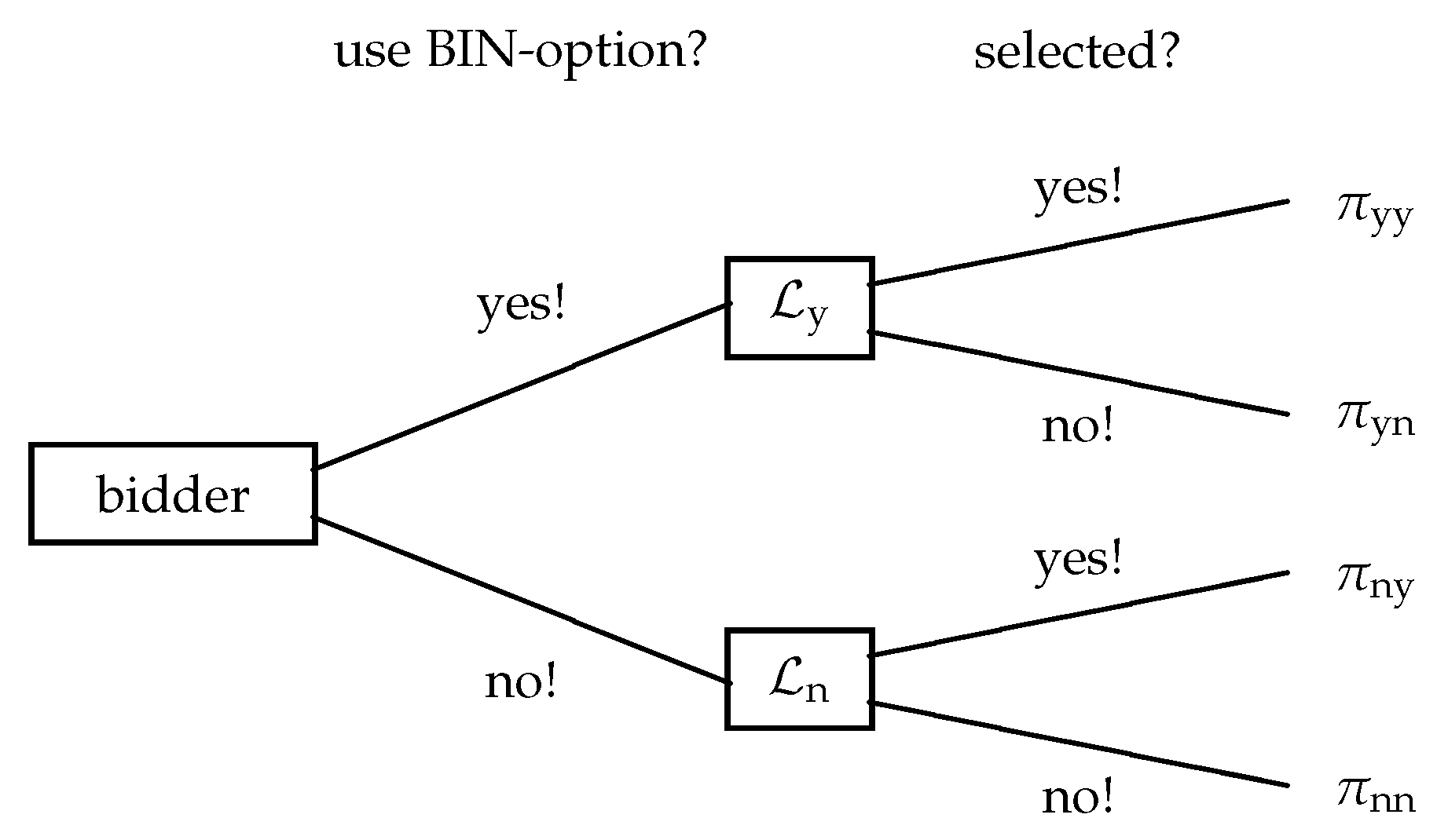
In the following, we summarize the key findings of the theoretical investigations into BIN options that apply to our experimental setup.8 While doing so, we assume that bidders are rational and maximize their monetary payoff (and that this is common knowledge). The bidder’s decision whether or not to select the BIN option is a choice between two lotteries (see Figure 1): ${\mathcal{L}}_{\mathrm{y}}$ (application for the option) and ${\mathcal{L}}_{\mathrm{n}}$ (no application for the option). An optimal decision depends on which of the two lotteries induces the highest expected utility.

In both lotteries, the bidder is decisive for the application of the BIN option with probability $\frac{1}{\#\mathrm{bidders}}$; with the residual probability, another bidder is decisive. With private values, bidding behavior in a potential subsequent auction is independent of the BIN application decisions. Therefore, it is a weakly-dominant strategy to submit the private valuation. This gives us the following hypothesis for our data.

Hypothesis 1. 

The resulting auction price is independent of the presence of a BIN option and the BIN price.

If a bidder is not decisive, her or his continuation payoff depends on the BIN application decisions of the other bidders and bidding behavior in the auction. As bidders decide upon BIN applications simultaneously, they cannot be influenced by the reference bidder’s application decision. However, as long as bidders follow the weakly-dominant strategy to submit their valuation in the auction, also bidding is unaltered by the reference bidder’s application decision. Hence, we get ${\pi }_{\mathrm{yn}}={\pi }_{\mathrm{nn}}$, and an optimal BIN decision for an expected utility maximizing individual depends on which of the two other continuation payoffs, ${\pi }_{\mathrm{yy}}$ or ${\pi }_{\mathrm{ny}}$, is higher.

For the reference bidder with private value v, the continuation payoff ${\pi }_{\mathrm{yy}}$ is equal to $v-p_B$, where $p_B$ denotes the prevailing BIN price. The continuation payoff ${\pi }_{\mathrm{ny}}$ is equal to the payoff of a standard auction, where it is a weakly-dominant strategy for every bidder to submit her or his private value. For the bidder, it is optimal to execute the BIN option if and only if the continuation payoff ${\pi }_{\mathrm{yy}}$ exceeds the continuation payoff ${\pi }_{\mathrm{ny}}$. In a situation with n bidders with private valuations that are identically and independently distributed via a differentiable cumulative distribution function F with support on the closed unit interval, this condition reads as follows.9

$${\pi }_{\mathrm{yy}}\ge {\pi }_{\mathrm{ny}}\iff v-p_B\ge v{F}^{n-1}\left(v\right)-{\int }_0^v{v}^{\prime }\mathrm{d}{F}^{n-2}\left(v^{\prime }\right).$$

By integration in parts, this can be shown to be equivalent to:

$$v-p_B\ge {\int }_0^v{F}^{n-1}\left(v^{\prime }\right)\mathrm{d}{v}^{\prime }\iff v-{\int }_0^v{F}^{n-1}\left(v^{\prime }\right)\mathrm{d}{v}^{\prime }\ge p_B.$$

The derivative of the left-hand side to v is $1-F^{n-1}\left(v\right)$, which is positive for all v. This means that the left-hand side is increasing in v. Hence, if a bidder is willing to accept a certain BIN price while having a certain value, she or he is willing to accept the BIN price when having an even higher value. Moreover, if a bidder with a certain value is willing to accept a certain BIN price, she or he is willing to accept any lower BIN price. These two properties together lead to the following hypothesis:

Hypothesis 2. 

A lower BIN price generates more applications for the BIN option.

In particular, in the experiment, at most one bidder (the one with the highest valuation) is expected to apply for the option with the high price, while at most two bidders (the two bidders with the highest valuations) are expected to apply for the option with a low price. In the former case, BIN executions do not lead to a loss in allocation efficiency; in the latter case, inefficiencies occur in case the BIN application of the second-highest valuation holder is effectuated. The subsequent auction in case the BIN option is not effectuated always results in an efficient allocation if bidders sticking to their weakly-dominant strategy.

Hypothesis 3. 

(i) Allocation efficiency in the high BIN treatment does not differ from allocation efficiency in the no BIN treatment. (ii) Allocation efficiency in the low BIN treatment is smaller than allocation efficiency in the no BIN treatment.

In the high BIN treatment, any execution of the BIN option leads to a revenue above the second-highest value (which is the equilibrium price in the auction). In the low BIN treatment, in contrast, any execution of the BIN option leads to a revenue below the second-highest value. Whether there are applications to the option, however, depends on the configuration of valuations and individual preferences. As some configurations of valuations are such that a risk-neutral profit-maximizing bidder should apply for the option (because the BIN price is below this bidder’s expectation of the auction price in case of a win), we expect to observe applications for the option and, therefore, also, executions. This leads to the following hypothesis:

Hypothesis 4. 

(i) Revenues in the high BIN treatment are above revenues in the no BIN treatment. (ii) Revenues in the no BIN treatment are above revenues in the low BIN treatment.

4. The Impact of BIN Options and Prices

Our experiment generates data of 300 trades (three treatments with ten independent bidder groups per treatment that interact in a sequence of ten auctions each). In this section, we compare auction efficiency and revenues and bidder behavior across treatments. For the statistical tests, we average the data of all rounds for each bidder group.10 This results in 30 independent observations; ten for each treatment. Each group within a given treatment faced different private values, and each configuration of values was used once in each treatment. For the analysis, we paired those groups with identical stimuli and used the Wilcoxon signed-rank test. If not indicated otherwise, the results that we report are significant at the 10% level in a two-sided test. The corresponding p-value is displayed as a subscript to the result of the two-sided test. When studying the effect of a BIN option on the subsequent auction, we aggregate the data over only those rounds where an auction resulted in all compared treatments. In all of these comparisons, we provide the number of auctions on which the analysis is based.

Hypothesis 3 suggests that efficiency depends on the presence and price of the option.

Table 1. Efficiency. Significance values result from Wilcoxon signed-rank tests with pairs of bidder groups as independent observations.

Treatment Comparison			Average $\mathrm{eff}$			Average $\#\mathrm{eff}$
No BIN	vs.	Low BIN	0.990	${>}_{0.004}$	0.944	0.88	${>}_{0.027}$	0.65
No BIN	vs.	High BIN	0.990	${\sim }_{0.375}$	0.993	0.88	${\sim }_{0.266}$	0.94
Low BIN	vs.	High BIN	0.944	${<}_{0.004}$	0.993	0.65	${<}_{0.004}$	0.94

presents the efficiency levels in the different treatments according to two different measures for efficiency ($\#\mathit{eff}$ and $\mathit{eff}$) and the test results of pairwise comparisons across the different treatments. $\#\mathit{eff}$ is the fraction of auctions that yields an efficient outcome. This measure is insensitive to the extent of potential efficiency losses. The second, alternative, measure takes into account to what extent efficiency is violated and reads $\mathit{eff}=\frac{v\left(\mathrm{winner}\right)}{v\left(\mathrm{highest}\right)}$ (the winner’s valuation divided by the highest valuation). In particular, $\mathit{eff}=1$ if the person with the highest value wins, and $\mathit{eff}=0$ if the winning subject does not value the good at all (in fact, $\frac{65}{135}$ would be the lowest possible value for $\mathit{eff}$ in our setup). The test results provide full support of Hypothesis 3.

Result 1. 

Allocation efficiency in the low BIN treatment is smaller than allocation efficiency in the no BIN and the high BIN treatment. There is no difference in allocation efficiency between the high BIN and the no BIN treatment.

The revenue to the seller in an auction is either the BIN price (in case of a successful BIN application by one of the bidders) or the final price in the auction.

Table 2. Revenue. Significance values result from Wilcoxon signed-rank tests with pairs of bidder groups as independent observations.

Treatment Comparison			Average Revenue
No BIN	vs.	Low BIN	109.48	${>}_{0.004}$	104.98
No BIN	vs.	High BIN	109.48	${>}_{0.049}$	108.01
Low BIN	vs.	High BIN	104.98	${<}_{0.010}$	108.01

presents the average revenues realized in the different treatments and the test result of pairwise comparisons across the different treatments. From these numbers, we can conclude that (1) the introduction of a BIN option has a negative impact on the seller’s revenue and (2) that a low BIN price gives rise to a lower revenue than a high BIN price. While the latter finding is in line with Hypothesis 4, the former result is only partially consistent, as the hypothesis that the high BIN treatment yields larger revenue compared to the no BIN treatment is rejected.

Result 2. 

The introduction of a temporary BIN option unambiguously reduces revenues, and revenues increase in the BIN price.

One factor that can explain the treatment comparison between the high BIN and the low BIN treatment is the execution of the BIN option, with the corresponding average BIN price being 115.06 in the high BIN treatment and 101.19 in the low BIN treatment.

Table 3. BIN applications.

Treatment	Number of Bidders Applying the BIN Option
	0	1	2	3	4	Total
No BIN	–	–	–	–	–	–
Low BIN	6	26	65	3	0	165
High BIN	39	60	1	0	0	62

summarizes the BIN applications made by the bidders in all 100 auctions (per treatment). On the basis of comparing the risk-neutral expected payoff from the auction given the private valuations (and given that opponents bid up to their valuation) with the payoff of an immediate gain by applying for the BIN option, we should observe 161 BIN applications in the low BIN treatment and 35 in the high BIN treatment. In this sense, the numbers in the table reflect some bidders being risk-averse or following simple heuristics, such as applying for the option whenever the private value is above the respective BIN price (which would generate 200 applications in the low BIN treatment and 100 in the high BIN treatment). As predicted by theory (Hypothesis 2), we find BIN option applications to be less frequent if the BIN price increases from low to high ($p<0.002$; two-sided Wilcoxon signed-rank with pairs of bidder groups as independent observations).

Result 3. 

The number of applications is significantly higher in the low BIN treatment than in the high BIN treatment.

The relatively low revenue in the low BIN treatments can therefore be attributed to more BIN option executions (and as a consequence, prices below the equilibrium in weakly-dominant strategies in the auction). However, the low revenue in the high BIN treatment relative to the no BIN treatment cannot be attributed to BIN executions (unless we frequently observed final prices above the second-highest value in the no BIN treatments, which is not the case): whenever the option gets executed in the high BIN treatments, it will yield higher revenues than in the weakly-dominant strategy equilibrium of the subsequent auction. This suggests that the (former) presence of an option affects bidding behavior in the subsequent auction.

Table 4. Average final auction prices. Significance values result from Wilcoxon signed-rank tests with pairs of bidder groups as independent observations.

Treatment Comparison			Number of Auctions	Average Price in the Auction
				Group Aggregation via Mean			Group Aggregation via Median
No BIN	vs.	Low BIN	51/100	112.12	${\sim }_{0.287}$	111.06	113.10	${\sim }_{0.285}$	112.25
No BIN	vs.	High BIN	84/100	110.12	${>}_{0.014}$	107.18	111.55	${>}_{0.029}$	107.15
Low BIN	vs.	High BIN	45/100	111.91	${>}_{0.002}$	108.87	112.65	${>}_{0.018}$	109.10

compares the average final auction prices across the treatments in a pairwise manner. For each pairwise comparison, we aggregated the data to the level of independent bidder groups. We only used those auction configurations for which the BIN option was not executed in either of the two respective treatments. The second column presents the number of auctions on which the comparisons are based. To control for outlier-driven results, we aggregated the rounds by the mean and the median (the results turn out to be robust). We do not find any significant difference in final auction prices between the no BIN treatment and the low BIN treatment, which is consistent with Hypothesis 1. In contrast to the theoretical prediction, however, we find that the prices resulting in the auction stage are significantly lower in the high BIN treatment compared to the no BIN treatment and the low BIN treatment.

Result 4. 

The price resulting in the auction is not independent of the BIN price: an unexecuted BIN option with a high price yields final auction prices below the final auction prices with a low BIN price and without a BIN option.

As indicated by Result 4, the poor revenue in auctions with a high BIN price can be attributed to the bidders’ reluctance to bid sufficiently competitively in this case. To further investigate this, we compare the number of bids above the respective BIN price in the two BIN option treatments against the comparable number in the treatment without the BIN option. The results are shown in

Table 5. Number of bids above the BIN price. Significance values result from Wilcoxon signed-rank tests with pairs of bidder groups as independent observations.

Treatment Comparison	Number of Auctions	Number of Final Bids Above BIN Price
No BIN vs. Low BIN	51/100	108 ${>}_{0.031}$ 95
No BIN vs. High BIN	84/100	47 ${>}_{0.047}$ 30

; in the second column, we display the number of auctions on which the comparison is based.

By the design of the BIN price in the treatments with the BIN option, we would expect to see 102 final bids above the BIN price in the low BIN treatment and 84 in the high BIN treatment. In both treatments, the number is below this theoretical benchmark and also below the experimental benchmark provided by the no BIN treatment. Hence, some bidders have been reluctant to bid more than they would have paid by executing the option.

Result 5. 

Final bids above a given BIN price are significantly more frequent in a no BIN treatment than in the corresponding BIN treatment.

5. Discussion

5.1. BIN as an Anchor (for What?)

The influence of a formerly present BIN option on final auction prices indicates that (some) bidders do not follow the weakly-dominant strategy to submit their private valuation to the bid agent.11 Hence, bidders either assign a different value to winning the auction or alter their bidding strategy in response to the former presence of a BIN option and its price. A simple reason for a “modified valuation” would be that bidders who did not apply for the option (and were decisive) feel regret for not having taken the opportunity and are reluctant to bid above a price that was at their disposal. To check for such “regret-histories”, we introduced a regret dummy for such cases and regressed the final proxy bid on it and the private value. The coefficient for the dummy is negative (which is in the right direction), but far from significant ($p=0.762$).12 Hence, an alteration of valuations by bidders who had been decisive and opted against the BIN option is not a likely explanation for the impact of a BIN option. However, this finding does not exclude regret that is unconditional on a bidder’s decisiveness with respect to BIN executions. Indeed, our experimental findings are in line with the hypothesis that bidders feel regret whenever the auction price exceeds the BIN price (no matter who started the auction) and, therefore, shade their bids compared to auctions without a BIN.

An alternative explanation for an influence of a BIN option on a bidder’s valuation could be that bidders take the seller’s utility into account and are reluctant to bid above the BIN price, because they do not want to “overpay”, e.g., an envious bidder would suffer from paying above the BIN price given that the BIN price is expected to be above the sellers own valuation. Would this be the way in which BIN options and their prices influence the bidders’ utility (and thereby bidding behavior), final auction prices in the low BIN treatment were to be below those in the high BIN treatment. As we saw in Table 4, this is not the case in our experiment.

Apart from such a direct impact of the former presence of a BIN option and its price on a bidder’s valuation, the private valuation environment of our experiment rules out any alterations of the bidder’s valuation that are based on the valuations of other bidders. However, it should not be taken for granted that bidders indeed ignore information such as a BIN price in a private value environment when they assess their opponents’ valuations. One particular important psychological bias discussed in the empirical literature, which suggests an influence of the BIN price, is anchoring. In their seminal article, Tversky and Kahneman (1965) [37] report an effect of the number displayed by a wheel of fortune on individuals’ estimates of the number of African countries in the United Nations. They systematize these findings with the heuristics of “anchoring and adjustment” for decision making under uncertainty. In an overview article, Chapman and Johnson (2002) [33] define an anchoring procedure as one in which “a salient but uninformative number is presented to subjects before they make a numerical judgement” in such a way that the uninformative number eventually influences the judgment. The authors thereby emphasize the importance of compatibility between the target information and the anchor.

In our experimental setting, the BIN price is implemented to be salient, but uninformative information for the subsequent bidding decision. The fact that final auction prices are not independent of the BIN price and bidders tend to truncate their bidding at the BIN price (while the option is not in effect anymore) suggests that subjects take more information into account than just their own private value when forming their bidding decision. Hence, the BIN price may serve as an anchor in the subsequent auction. The question is: an anchor for what? Is it used to update the own valuation, or may it be used to update beliefs about the other bidders’ valuations? Additionally, in the case of the latter, why would it still affect bidding behavior in an English auction where bidding up to one’s own valuation is a weakly-dominant strategy? As we implemented a setting without any uncertainty regarding one’s own valuation, it is not plausible to expect bidders to update their own valuation using the BIN price.13

We know from recent studies on over- and under-bidding in second-price auctions that information about other bidders’ values indeed influences bidding decisions. Andreoni et al. (2007) [31] and Cooper and Fang (2008) [34] show that bidders tend to bid more fiercely if their own value is close to the value of another bidder. The authors attribute this pattern to spiteful behavior (bidders want to raise the price a bidder holding a higher value has to pay) or the “joy-of-bidding” (bidders regard winning an auction against a strong opponent as more valuable). In contrast, Kamecke (1999) [36] observes in an English auction with two bidders who know in advance the identity of the bidder with the higher valuation that bidders collude such that the bidder with the lower valuation does not bid up to his or her private value. He explains this sort of underbidding with efficiency concerns among the bidders who do not take the seller (or experimenter) into account. Similarly, bidders could also use information about their opponents’ values for an estimation of their own winning probability and decide whether bidding is worthwhile in the first place.

To distinguish between these different channels by which information on other bidders’ valuations may influence bidding and a BIN option may serve as an anchor, we compare the final bids of the second-highest value holders for the low BIN and the high BIN treatments.14 If bidders indeed take the BIN price as an anchor for the other bidders’ values, spiteful behavior or “joy-of-winning” would lead to higher bids for a high BIN price than for a low BIN price. If, in contrast, bidders take the BIN price as an anchor for the probability to win the auction or try to collude, a higher BIN price may well lead to earlier drop-outs and lower final bids. An examination of the data using the Wilcoxon signed-rank test (two-sided) on the basis of group averages (independent observations) lends support for the latter hypothesis. While the final bids of the second-highest value holders in the low BIN treatment are not significantly different from their values ($p=0.375$), the second-highest value holders in the high BIN treatment systematically underbid ($p=0.002$) by 2.09 ECU on average. Moreover, their final bids are significantly lower in the high BIN than in the low BIN treatment ($p=0.010$).

5.2. Role of Bidding Experience

Behavior seems to be rather stable over the 10 rounds of our experiment. In Appendix B, we report the results of our analysis restricted to the last five rounds and observe the same pattern regarding efficiency (see

Table B1. Efficiency. Significance values result from Wilcoxon-signed rank tests with pairs of bidder groups as independent observations.

Treatment Comparison			Average $\mathrm{eff}$			Average$\#\mathrm{eff}$
No BIN	vs.	Low BIN	0.997	${>}_{0.016}$	0.968	0.90	${>}_{0.094}$	0.70
No BIN	vs.	High BIN	0.997	${\sim }_{0.813}$	0.995	0.90	${\sim }_{0.813}$	0.94
Low BIN	vs.	High BIN	0.968	${\sim }_{0.055}$	0.995	0.70	${<}_{0.047}$	0.94

) and revenue (see

Table B2. Revenue. Significance values result from Wilcoxon signed-rank tests with pairs of bidder groups as independent observations.

Treatment Comparison			Average Revenue
No BIN	vs.	Low BIN	110.14	${>}_{0.002}$	105.10
No BIN	vs.	High BIN	110.14	${>}_{0.084}$	108.54
Low BIN	vs.	High BIN	105.10	${<}_{0.012}$	108.54

). Furthermore, we do not observe a time trend in the number of BIN applications (see Figure B1), which supports our hypothesis that participants do not learn the construction of BIN prices. With respect to final auction prices, we still detect significantly higher prices in the no BIN compared to the high BIN treatment. Interestingly, we now also observe significantly lower prices in the low BIN compared to the no BIN treatment (and no longer a difference between final auction prices in the low and the high BIN treatment) (see

Table B3. Average final auction prices. Significance values result from Wilcoxon signed-rank tests with pairs of bidder groups as independent observations.

Treatment Comparison			Number of Auctions	Average Price in the Auction
				Group Aggregation via Mean			Group Aggregation via Median
No BIN	vs.	Low BIN	28/50	112.54	${>}_{0.020}$	109.43	111.55	${>}_{0.051}$	108.20
No BIN	vs.	High BIN	41/50	110.73	${>}_{0.020}$	107.68	109.10	${>}_{0.078}$	106.05
Low BIN	vs.	High BIN	25/50	109.72	${\sim }_{0.910}$	108.56	107.20	${\sim }_{0.895}$	106.30

). Only when looking at the number of bids above a BIN price, the number for no BIN treatments (25) is no longer significantly different from the number for high BIN treatments (17). These findings suggest that our results are rather robust to bidding experience in our setup.

5.3. Design Implications

Trading with an auction that includes a BIN option has become increasingly popular for online market places. For standard textbook auction theory with monopolistic sellers and risk-neutral bidders who are patient and have independent private values, this popularity is difficult to explain as an auction with an (optimally chosen) reservation price resembles a revenue-maximizing mechanism. However, as soon as bidders are risk averse or impatient, their willingness to pay in a fixed price transaction exceeds the corresponding willingness to pay in an auction, and this “fixed price premium” can be exploited by sellers who offer trade at a fixed price or a BIN option (see Matthews and Katzmann, 2006 [29], or Shariar and Wooders, 2011 [27]). Fixed prices or BIN options may also be a good design tool for sellers who face competition by sellers of the same or similar products (see Bauner, 2015 [32]) as it helps buyers to coordinate on different sellers. Additionally, a fixed price or BIN price can be considered as a signal of the seller’s own valuation in an environment with affiliated values (see Li et al., 2009 [26]). Therefore, while the previous literature suggests a revenue-enhancing role for (optimally chosen) BIN options, our experiment demonstrates that such an optimal BIN price choice may not only rely on an accurate assessment of bidders’ valuations, risk attitudes or time preferences, but also has to take cognitive biases into account.

References

1. Cheema, A.; Chakravarti, D.; Sinha, A. Bidding behavior in descending and ascending auctions. Mark. Sci. 2012, 31, 779–800. [Google Scholar] [CrossRef]
2. eBay Inc. eBay Inc. Reports Strong Fourth Quarter and Full Year 2011 Results; eBay Inc.: San Jose, CA, USA, 2012. [Google Scholar]
3. eBay Inc. eBay Inc. Reports Strong Fourth Quarter and Full Year 2012 Results; eBay Inc.: San Jose, CA, USA, 2013. [Google Scholar]
4. Lucking-Reiley, D. Using field experiments to test equivalence between auction formats: Magic on the Internet. Am. Econ. Rev. 1999, 89, 1063–1080. [Google Scholar] [CrossRef]
5. Houser, D.; Wooders, J. Reputation in auctions: Theory, and evidence from eBay. J. Econ. Manag. Strategy 2006, 15, 353–369. [Google Scholar] [CrossRef]
6. Ariely, D.; Simonson, I. Buying, bidding, playing or competing? Value assessment and decision dynamics in online auctions. J. Consum. Psychol. 2003, 13, 113–123. [Google Scholar] [CrossRef]
7. Bajari, P.; Hortaçsu, A. The winner’s curse, reserve prices, and endogenous entry: Empirical insights from eBay auctions. RAND J. Econ. 2003, 34, 329–355. [Google Scholar]
8. Häubl, G.; Leszczyc, P.P. Minimum Prices and Product Valuations in Auctions; Marketing Science Institute Report 03-117; Marketing Science Institute: Cambridge, MA, USA, 2003. [Google Scholar]
9. Kamins, M.; Dréze, X.; Folkes, V. A field study of the effects of minimum and reserve prices on Internet auctions. J. Consum. Res. 2004, 30, 622–628. [Google Scholar]
10. Haruvy, E.; Leszczyc, P.P. The impact of online auction duration. Decis. Anal. 2010, 7, 99–106. [Google Scholar]
11. Roth, A.; Ockenfels, A. Late-minute bidding and the rules for ending second-price auctions: Evidence from eBay and Amazon on the Internet. Am. Econ. Rev. 2002, 92, 1093–1103. [Google Scholar]
12. Ariely, D.; Ockenfels, A.; Roth, A. An experimental analysis of ending rules in Internet auctions. RAND J. Econ. 2005, 36, 890–907. [Google Scholar]
13. Ockenfels, A.; Roth, A. Late and multiple bidding in second price Internet auctions: Theory and evidence concerning different rules for ending an auction. Games Econ. Behav. 2006, 55, 297–320. [Google Scholar]
14. Lee, H.; Malmendier, U. The bidder’s curse. Am. Econ. Rev. 2011, 101, 749–787. [Google Scholar]
15. Haruvy, E.; Leszczyz, P.P. Internet auctions. Found. Trends Mark. 2009, 4, 1–75. [Google Scholar]
16. Park, Y.-H.; Bradlow, E. An integrated model for bidding behavior in Internet auctions: Whether, who, when, and how much. J. Mark. Res. 2005, 42, 470–482. [Google Scholar]
17. Durham, Y.; Roelofs, M.; Standifird, S. EBay’s buy it-now function: Who, when, and how. Top. Econ. Anal. Policy 2004, 4, 1–22. [Google Scholar]
18. Hendricks, K; Onur, I.; Wiseman, T. Preemption and Delay in eBay Auctions; University of Texas at Austin Working Paper; University of Texas at Austin: Austin, TX, USA, 2005. [Google Scholar]
19. Dodonova, A.; Koroshilov, Y. Anchoring and transaction utility: Evidence from on-line auctions. Appl. Econ. Lett. 2004, 11, 307–310. [Google Scholar]
20. Wang, X.; Montgomery, A.; Srinivasan, K. When auction meets fixed price: A theoretical and empirical examination of buy-it-now auctions. Quant. Mark. Econ. 2008, 6, 339–370. [Google Scholar]
21. Rochet, J.-C.; Tirole, J. Two-sided markets: A progress report. RAND J. Econ. 2006, 37, 645–667. [Google Scholar]
22. Chan, T.; Kadiyali, V.; Park, Y. Willingness to pay and competition in online auctions. J. Mark. Res. 2007, 44, 324–333. [Google Scholar]
23. Yao, S.; Mela, C. Online auction demand. Mark. Sci. 2008, 27, 861–885. [Google Scholar]
24. Haruvy, E.; Leszczyz, P.P. Search and choice in online consumer auctions. Mark. Sci. 2010, 29, 1152–1164. [Google Scholar]
25. Zeithammer, R. Forward-looking bidding in auctions. J. Mark. Res. 2006, 63, 462–476. [Google Scholar]
26. Li, S.; Srinivasan, K.; Sun, B. Internet auction features as quality signals. J. Mark. 2009, 73, 75–92. [Google Scholar]
27. Shahriar, Q.; Wooders, J. An experimental study of auctions with a buy price under private and common values. Games Econ. Behav. 2011, 72, 558–573. [Google Scholar]
28. Budish, E.; Takeyama, L. Buy prices in online auctions: Irrationality on the Internet? Econ. Lett. 2001, 73, 325–333. [Google Scholar]
29. Matthews, T.; Katzmann, B. The role of varying risk attitudes in an auction with a buyout option. Econ. Theory 2006, 27, 597–613. [Google Scholar]
30. Reynolds, S.; Wooders, J. Auctions with a buy-price. Econ. Theory 2006, 38, 9–39. [Google Scholar]
31. Andreoni, J.; Che, Y.; Kim, J. Asymmetric information about rival’s types in standard auctions: An experiment. Games Econ. Behav. 2007, 59, 240–259. [Google Scholar]
32. Bauner, C. Mechanism choice and the buy-it-now auction: A structural model of competing buyers and sellers. Int. J. Ind. Organ. 2015, 38, 9–31. [Google Scholar]
33. Chapman, G.; Johnson, E. Incorporating the irrelevant: Anchors in judgments of belief and value. In The Psychology of Intuitive Judgement: Heuristics and Biases; Gilovich, T., Griffin, D., Kahneman, D., Eds.; Cambridge University Press: Cambridge, UK, 2002. [Google Scholar]
34. Cooper, D.; Fang, H. Understanding overbidding in second price auctions: An experimental study. Econ. J. 2008, 118, 1572–1595. [Google Scholar]
35. Fischbacher, U. z-Tree—Zurich toolbox for readymade economic experiments: Experimenter’s manual. Exp. Econ. 2007, 10, 171–178. [Google Scholar]
36. Kamecke, U. Competition, Cooperation and Envy in a Simple English Auction; Mimeo, Humboldt-University Berlin: Berlin, Germany, 1999. [Google Scholar]
37. Tversky, A.; Kahneman, D. Judgment under uncertainty: Heuristics and biases. Science 1965, 185, 1124–1131. [Google Scholar]
Figure 1. The buy-it-now (BIN) decision is a choice between lotteries.
Games 07 00008 g001