
Process Simulation for the Design and Scale Up of Heterogeneous Catalytic Process: Kinetic Modelling Issues


Abstract
:
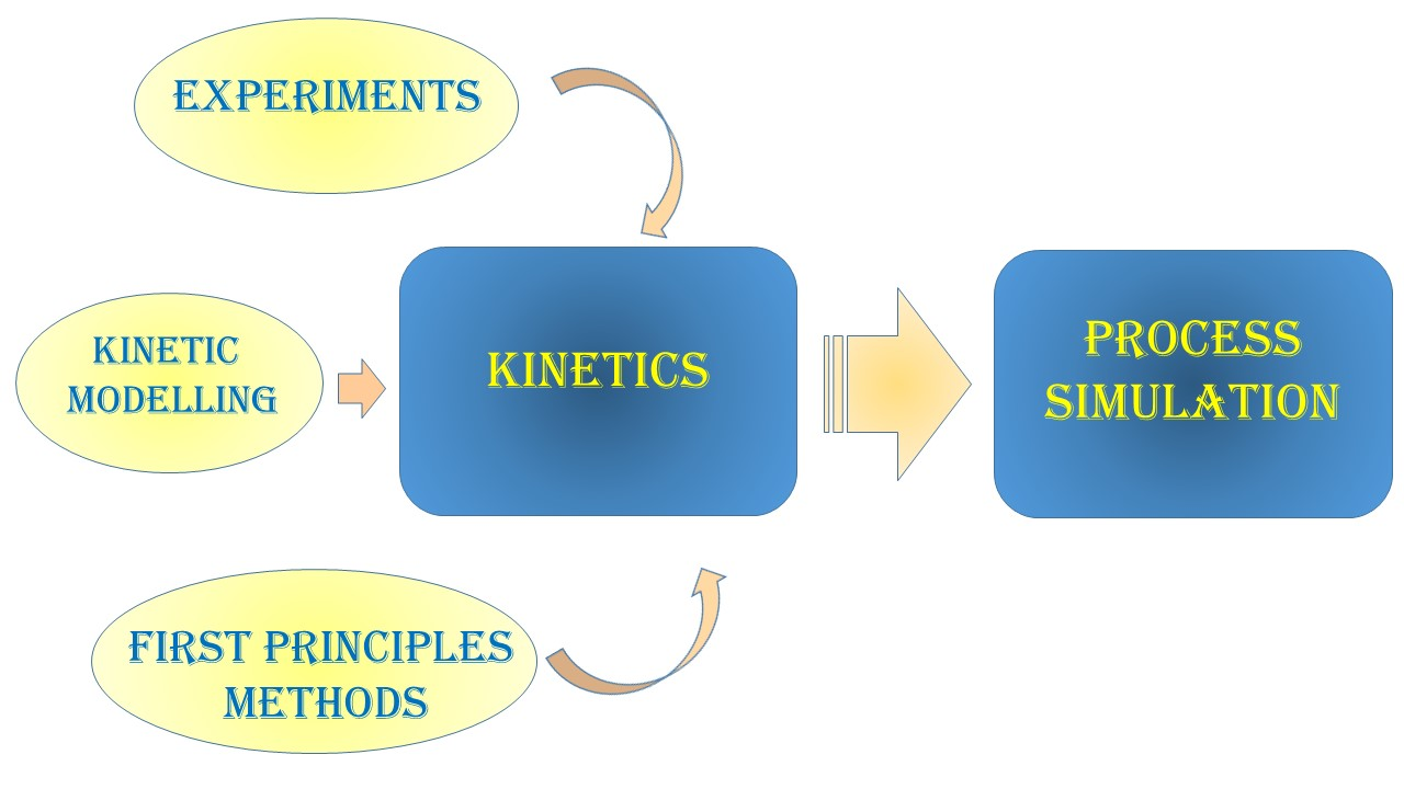
1. Introduction: How to Implement Kinetic Models into Process Simulators
- (1)
- Process simulation is a key step for process design;
- (2)
- Reactive systems need the definition of a reaction set with the relative kinetic parameters in a well standardized form, essentially the same for the different process simulators;
- (3)
- For some relatively simple, yet very important systems, the literature available on kinetic description is already suitable for a direct implementation into the process simulator (examples are reported in the following for ammonia and methanol synthesis);
- (4)
- When kinetic models are not available in this form, suitable kinetic data should be regressed again in the needed form for implementation in the process simulator;
- (5)
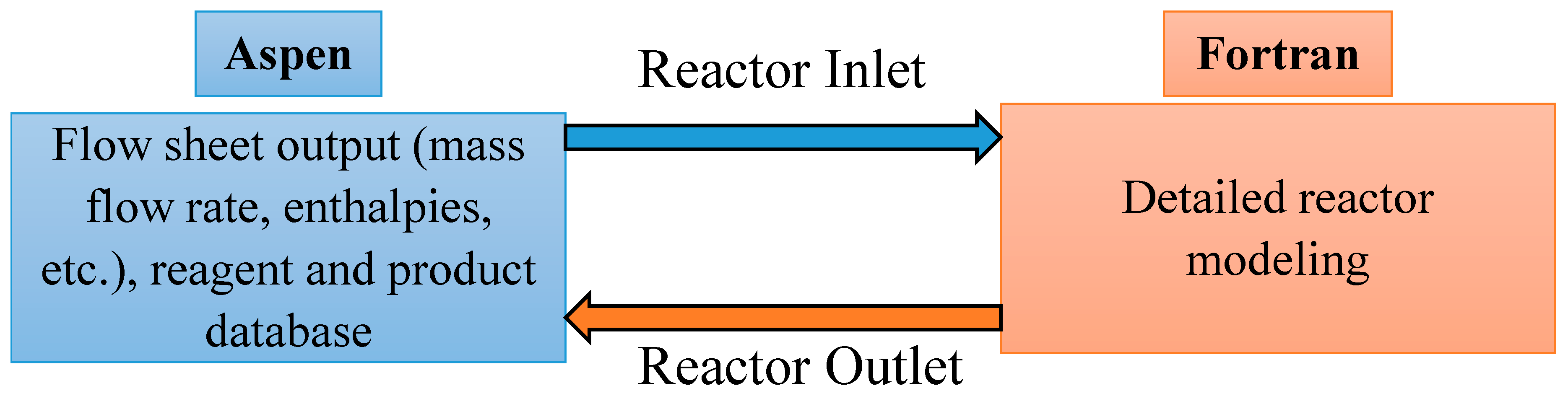
- In case particular kinetic equations are specifically needed, differing from the LHHW model, user models can be implemented in external subroutines and recalled by the simulator;
- (6)
- When the reaction set complexity becomes too high, lumped kinetic models are no more useful, because the powerful aid of the simulator is the prediction of plant performance under widely varied conditions. Empirical models are also at risk from this point of view. Therefore, microkinetic modelling allows the simulator to reliably follow the system performance;
- (7)
- Again, if the amount of parameters to be determined in a microkinetic scheme becomes too high, high correlation among them is usually observed and predictions reliability is newly at risk. Therefore, especially in such cases, the possibility of independently determining some of the required kinetic parameters through ab initio methods is a powerful tool to cope with this issue.
1.1. Methanol Synthesis
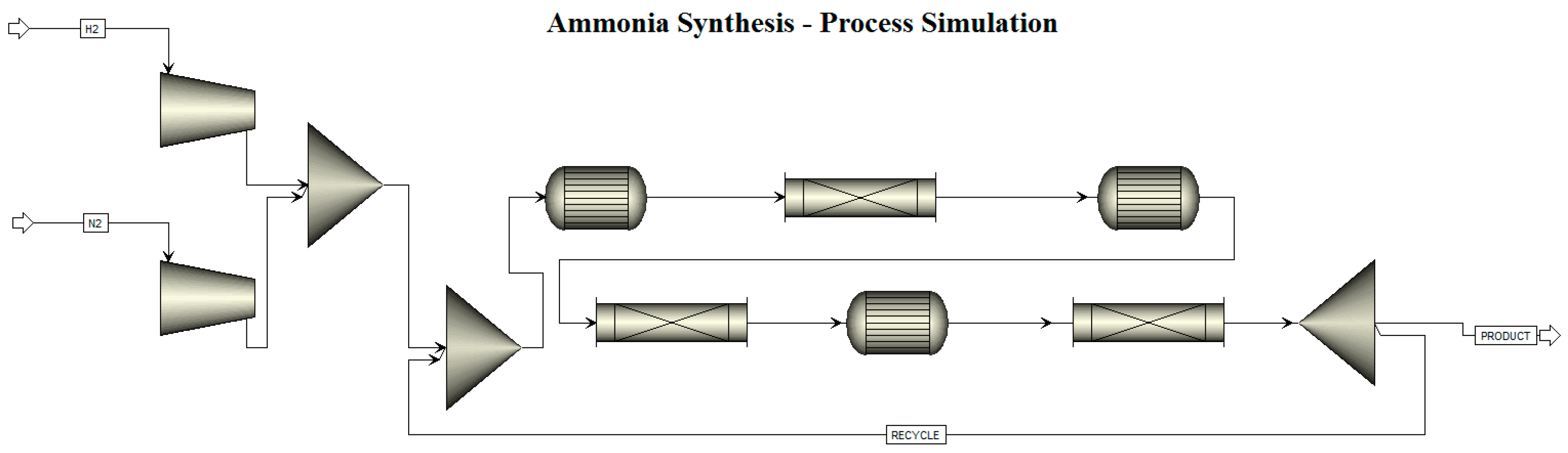
1.2. Ammonia Synthesis
1.3. Effect of Transport Phenomena
1.4. User Defined Models
2. Processes Following Complex Kinetic Schemes
2.1. Simulations of Reforming Processes
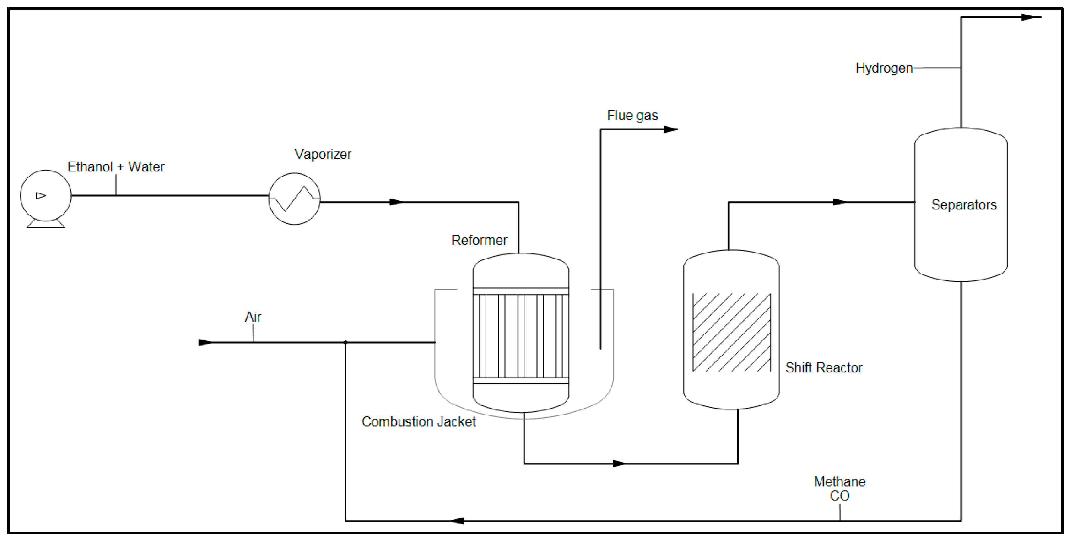
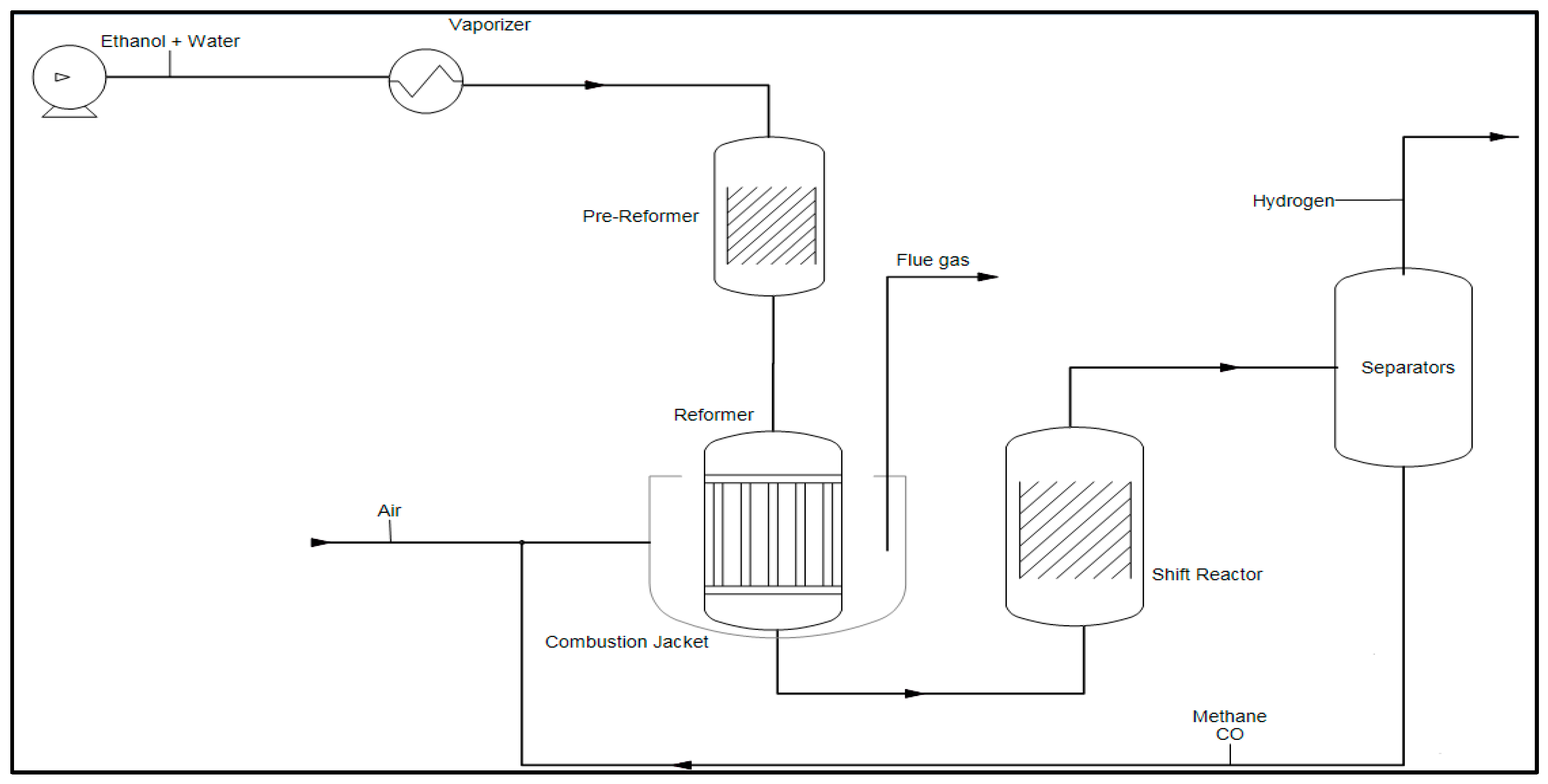
Hydrogen Production by Steam Reforming
2.2. Kinetic and Theoretical Analysis of Ethanol Reforming
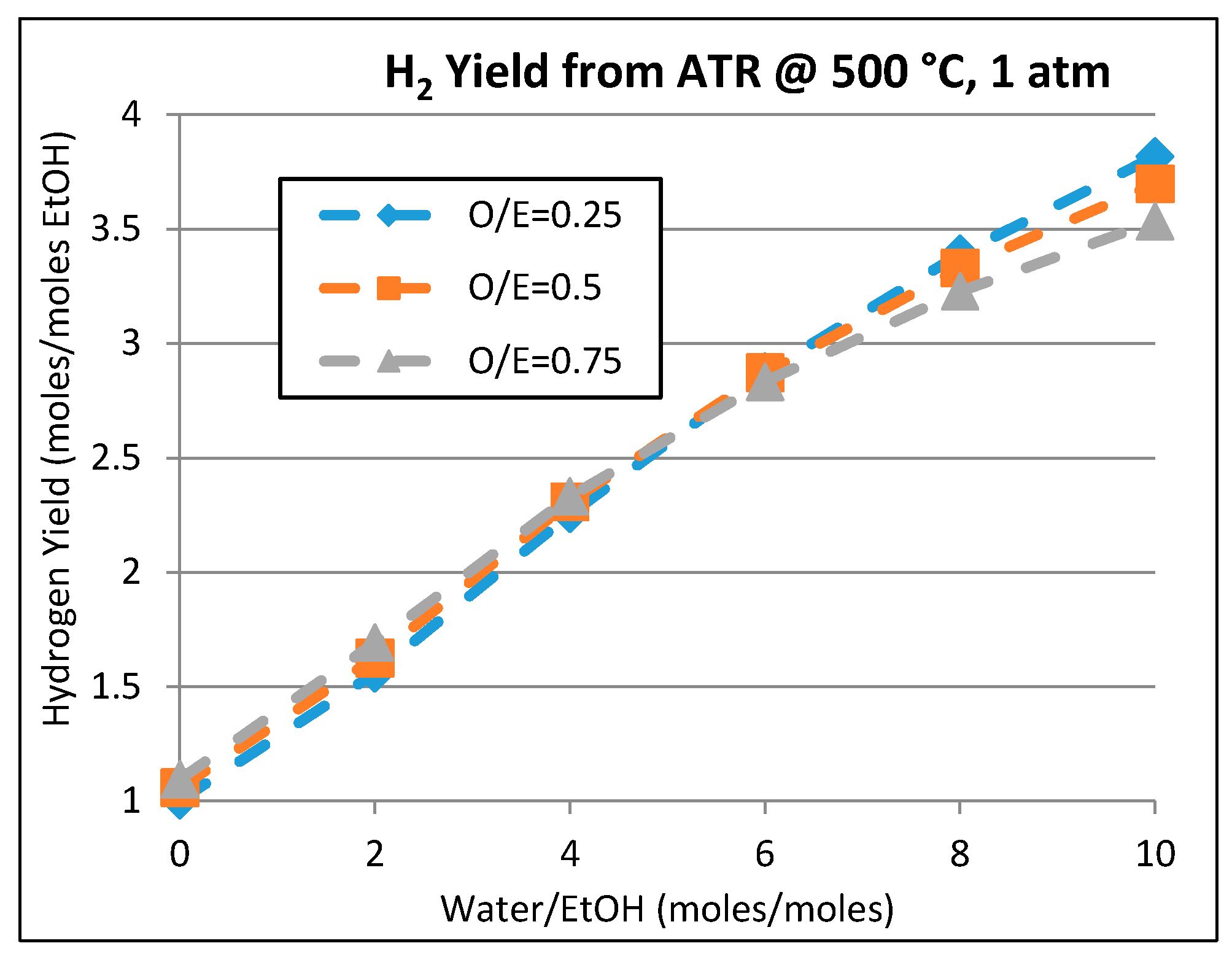
2.2.1. ESR: Conversion Rates and Steady States
2.2.2. ESR: From Stoichiometry to Mechanism
2.2.3. Other Reforming Models
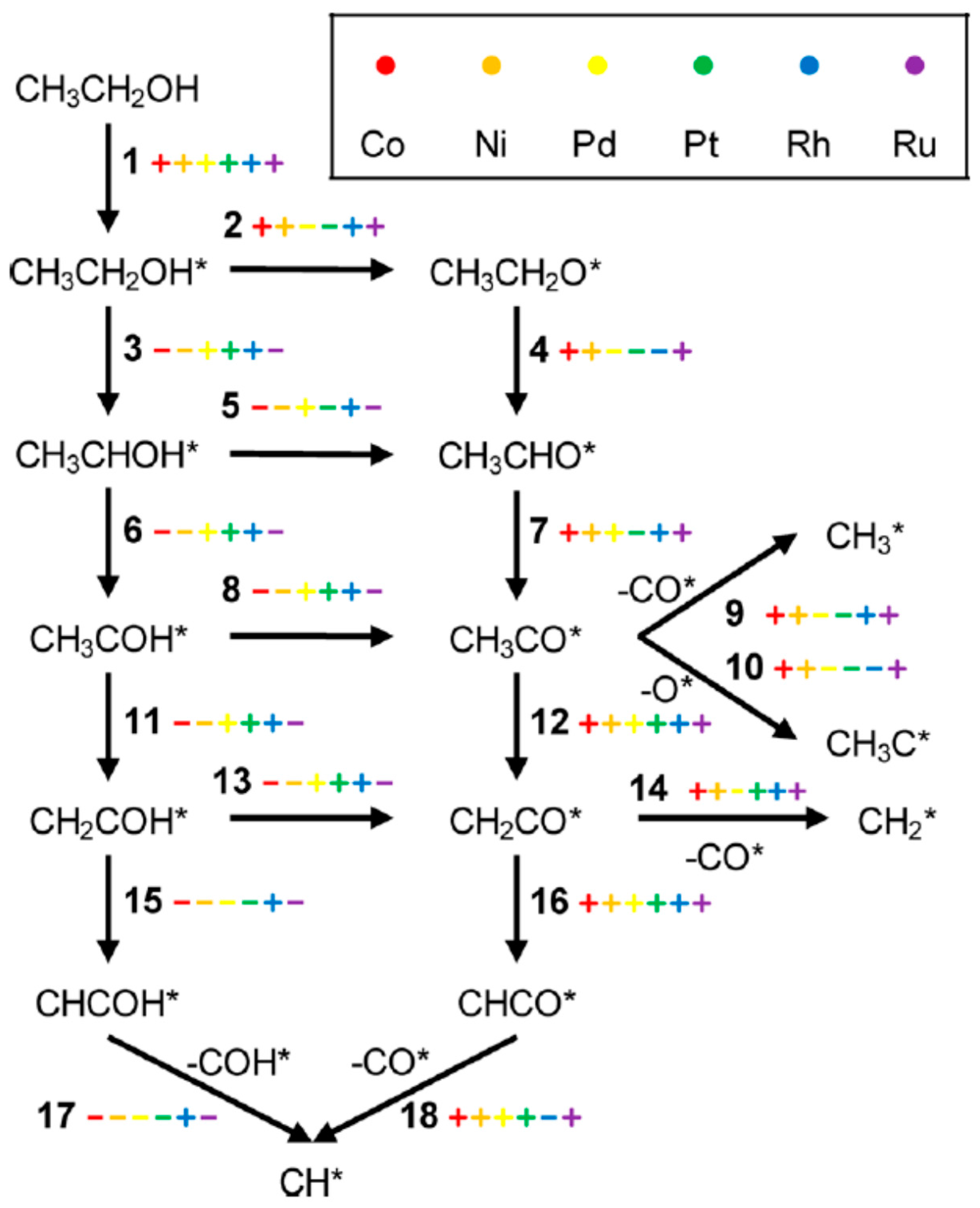
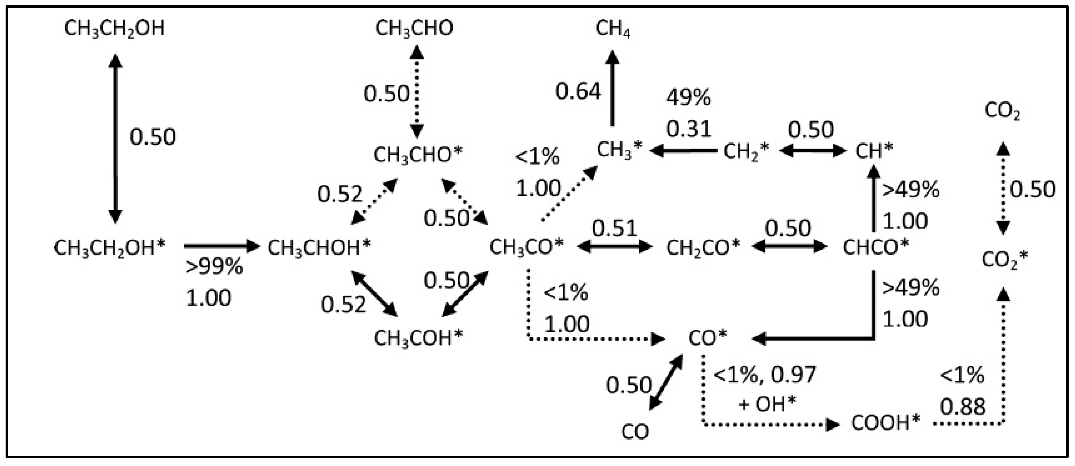
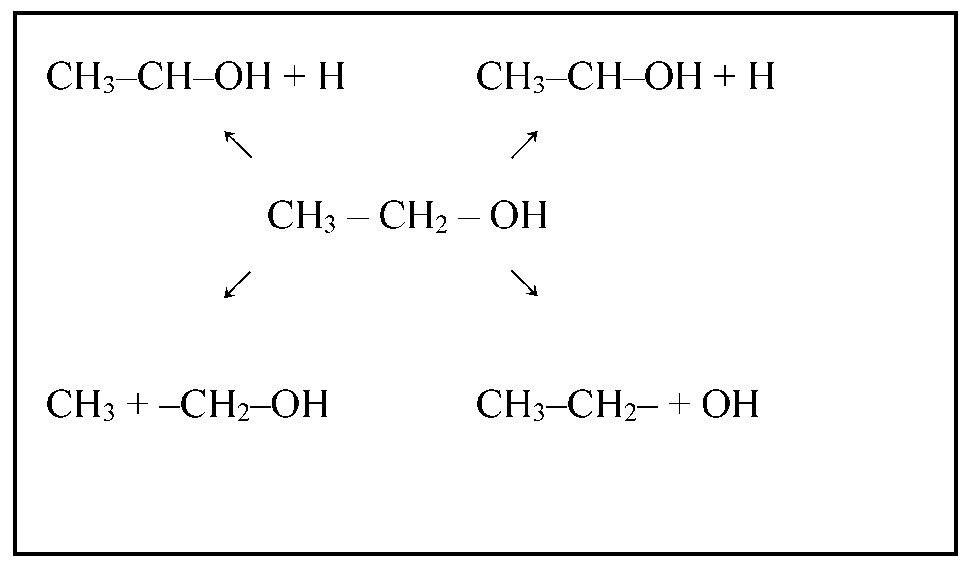
2.2.4. ESR: From Chemical Bonds to Hydrogen
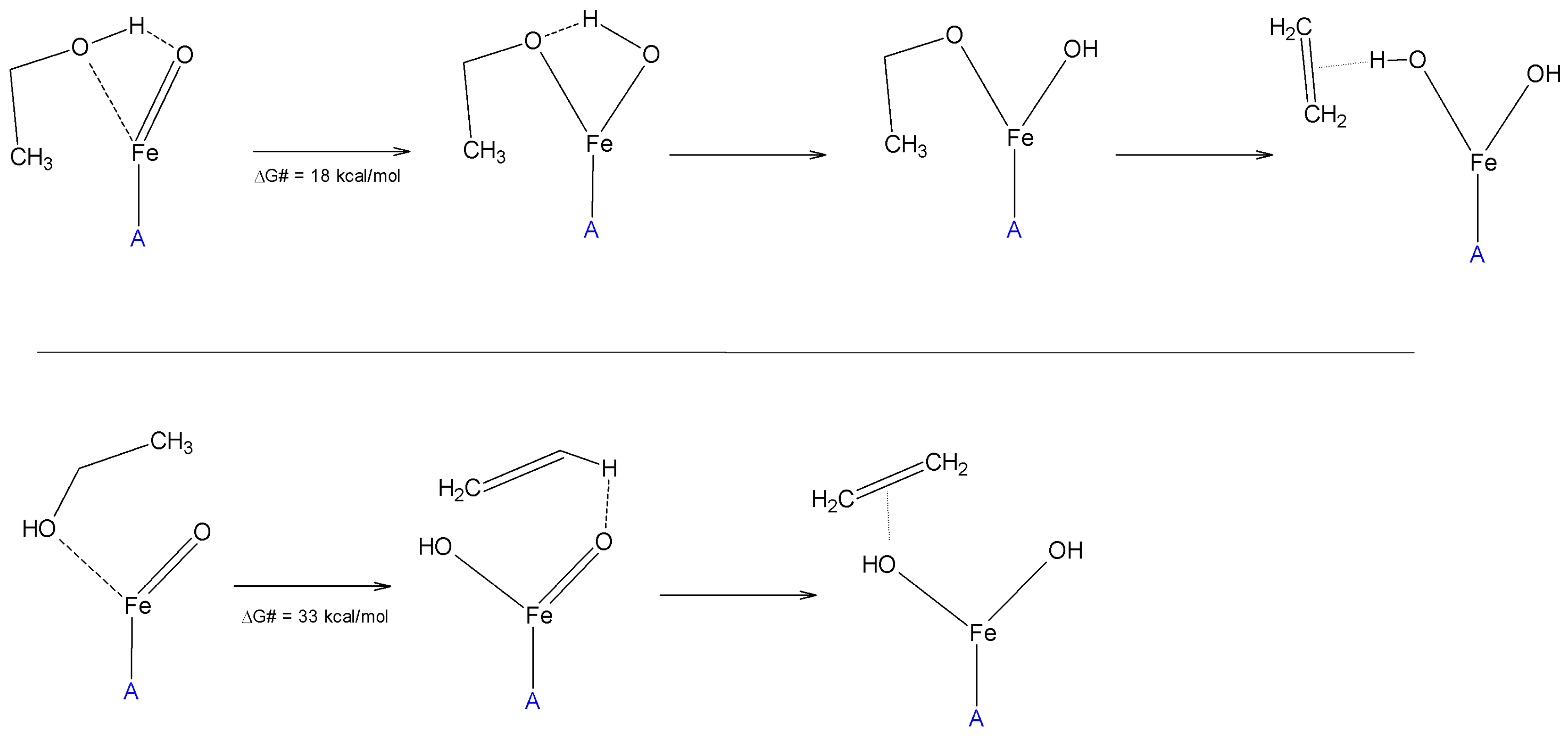
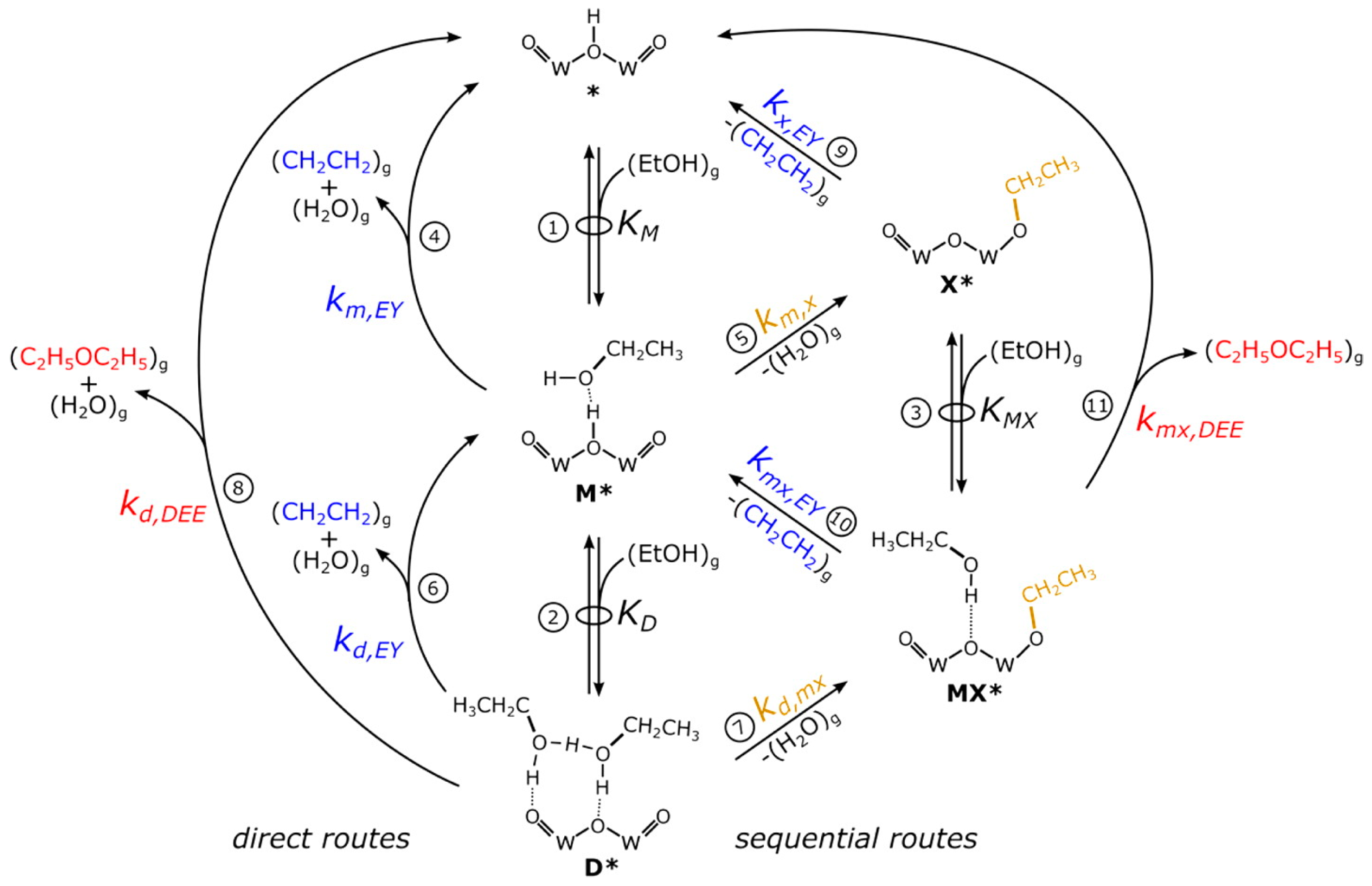
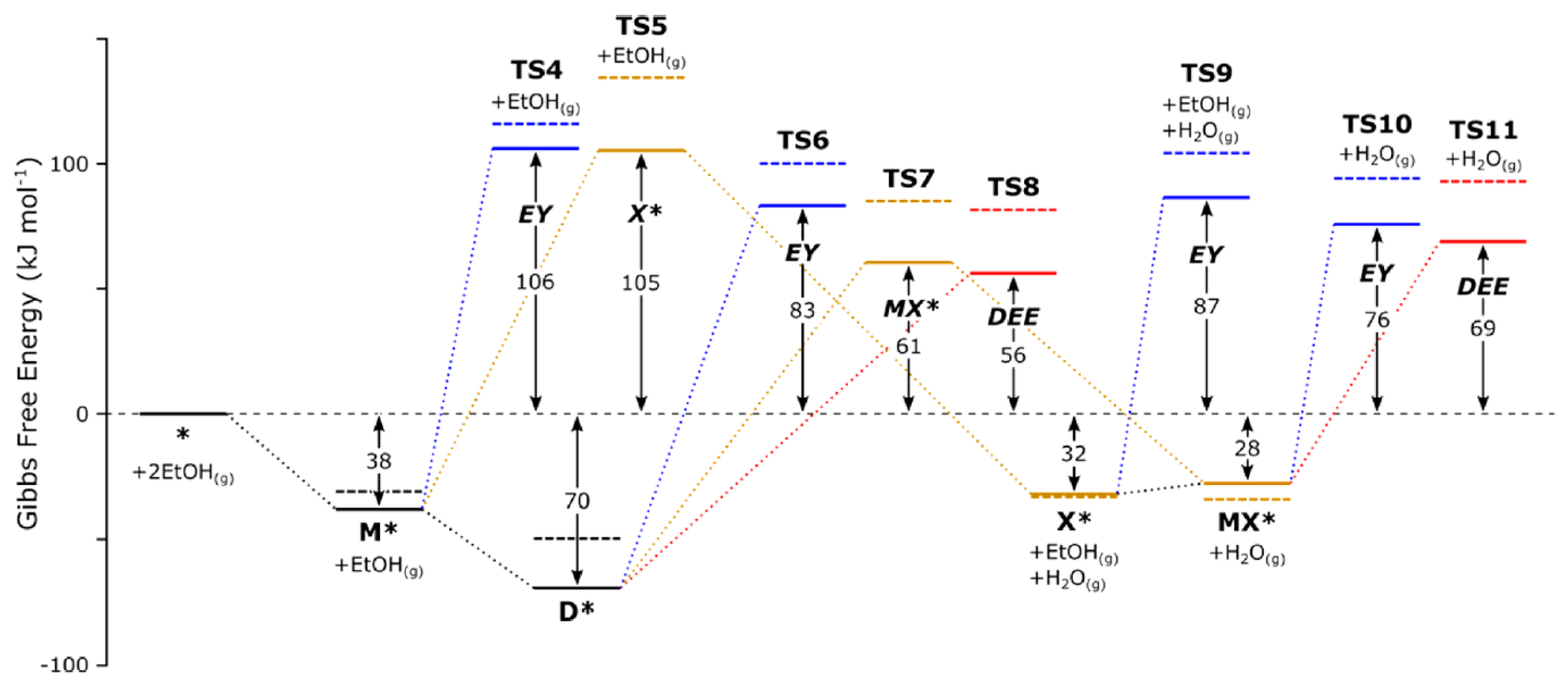
2.3. Ethanol to Ethylene
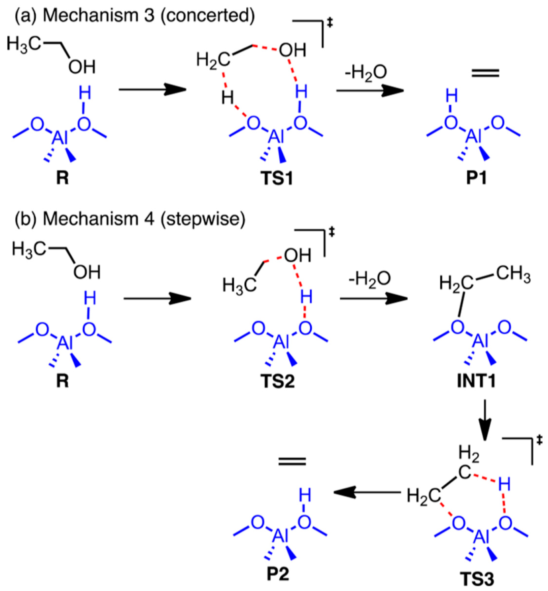
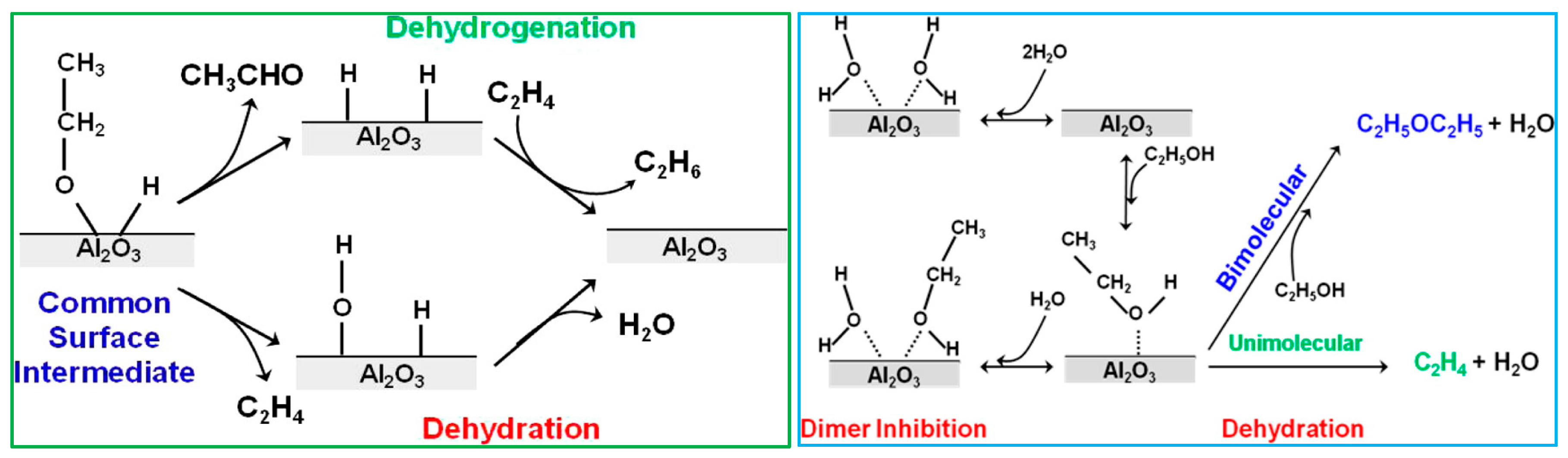
2.3.1. Ethanol to Ethylene: Direct Dehydration
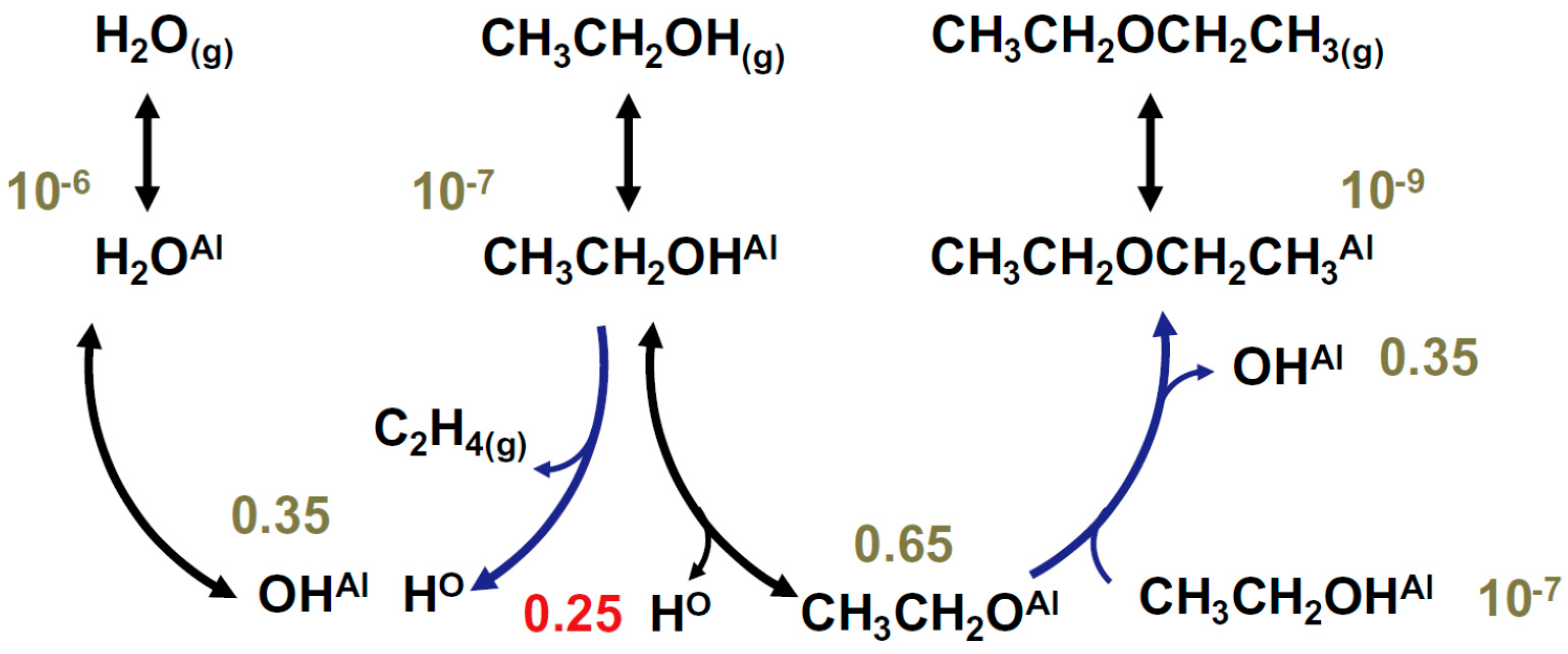
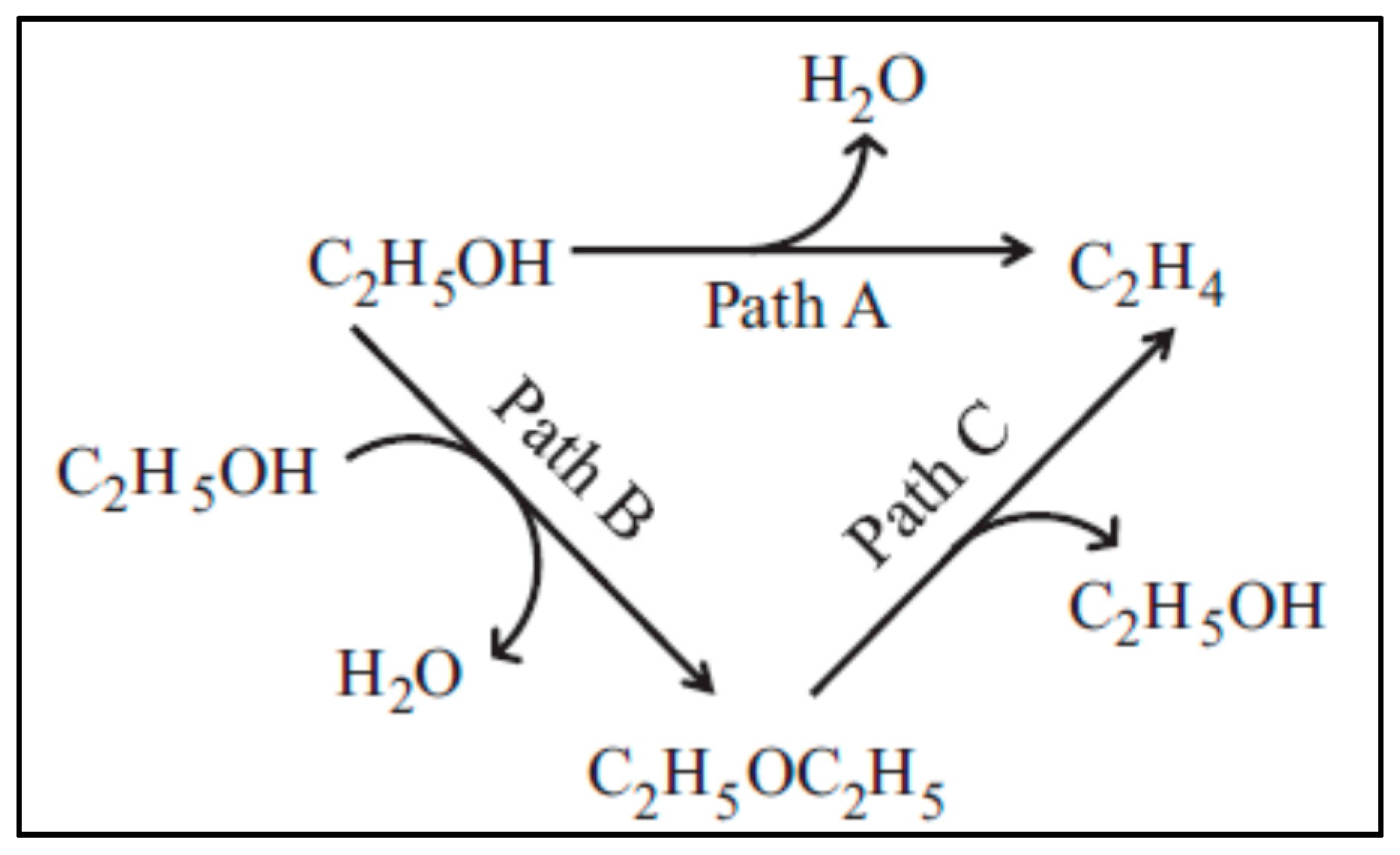
2.3.2. Ethanol to Ethylene: Parallel Paths
3. Conclusions
Author Contributions
Conflicts of Interest
References
- Luyben, W.L. Design and Control of a Methanol Reactor/Column Process. Ind. Eng. Chem. Res. 2010, 49, 6150–6163. [Google Scholar] [CrossRef]
- Vanden Bussche, K.M.; Froment, G.F. A Steady-State Kinetic Model for Methanol Synthesis and the Water Gas Shift Reaction on a Commercial Cu/ZnO/Al2O3Catalyst. J. Catal. 1996, 161, 1–10. [Google Scholar] [CrossRef]
- Van-Dal, É.S.; Bouallou, C. Design and simulation of a methanol production plant from CO2 hydrogenation. J. Clean. Prod. 2013, 57, 38–45. [Google Scholar] [CrossRef]
- Lim, H.-W.; Park, M.-J.; Kang, S.-H.; Chae, H.-J.; Bae, J.W.; Jun, K.-W. Modeling of the kinetics for methanol synthesis using Cu/ZnO/Al2O3<ZrO2 catalyst: Influence of carbon dioxide during hydrogenation. Ind. Eng. Chem. Res. 2009, 48, 10448–10455. [Google Scholar] [CrossRef]
- Zhang, C.; Jun, K.W.; Gao, R.; Kwak, G.; Park, H.G. Carbon dioxide utilization in a gas-to-methanol process combined with CO2/Steam-mixed reforming: Techno-economic analysis. Fuel 2017, 190, 303–311. [Google Scholar] [CrossRef]
- Matzen, M.; Alhajji, M.; Demirel, Y. Chemical storage of wind energy by renewable methanol production: Feasibility analysis using a multi-criteria decision matrix. Energy 2015, 93, 343–353. [Google Scholar] [CrossRef]
- Iyer, S.S.; Renganathan, T.; Pushpavanam, S.; Vasudeva, K.M.; Kaisare, N. Generalized thermodynamic analysis of methanol synthesis: Effect of feed composition. J. CO2 Util. 2015, 10, 95–104. [Google Scholar] [CrossRef]
- Rossetti, I.; Pernicone, N.; Ferrero, F.; Forni, L. Kinetic study of ammonia synthesis on a promoted Ru/C catalyst. Ind. Eng. Chem. Res. 2006, 45, 4150–4155. [Google Scholar] [CrossRef]
- Rossetti, I.; Pernicone, N.; Forni, L. Graphitised carbon as support for Ru/C ammonia synthesis catalyst. Catal. Today 2005, 102–103, 219–224. [Google Scholar] [CrossRef]
- Pernicone, N.; Ferrero, F.; Rossetti, I.; Forni, L.; Canton, P.; Riello, P.; Fagherazzi, G.; Signoretto, M.; Pinna, F. Wustite as a new precursor of industrial ammonia synthesis catalysts. Appl. Catal. A Gen. 2003, 251, 121–129. [Google Scholar] [CrossRef]
- Rossetti, I.; Pernicone, N.; Forni, L. Promoters effect in Ru/C ammonia synthesis catalyst. Appl. Catal. A Gen. 2001, 208, 271–278. [Google Scholar] [CrossRef]
- Yu, B.Y.; Chien, I.L. Design and Economic Evaluation of a Coal-Based Polygeneration Process to Coproduce Synthetic Natural Gas and Ammonia. Ind. Eng. Chem. Res. 2015, 54, 10073–10087. [Google Scholar] [CrossRef]
- Arora, P.; Hoadley, A.F.A.; Mahajani, S.M.; Ganesh, A. Small-Scale Ammonia Production from Biomass: A Techno-Enviro-Economic Perspective. Ind. Eng. Chem. Res. 2016, 55, 6422–6434. [Google Scholar] [CrossRef]
- Andersson, J.; Lundgren, J. Techno-economic analysis of ammonia production via integrated biomass gasification. Appl. Energy 2014, 130, 484–490. [Google Scholar] [CrossRef]
- Aráujo, A.; Skogestad, S. Control structure design for the ammonia synthesis process. Comput. Chem. Eng. 2008, 32, 2920–2932. [Google Scholar] [CrossRef]
- Mostafavi, E.; Sedghkerdar, M.H.; Mahinpey, N. Thermodynamic and Kinetic Study of CO2 Capture with Calcium Based Sorbents: Experiments and Modeling. Ind. Eng. Chem. Res. 2013, 52, 4725–4733. [Google Scholar] [CrossRef]
- Abdelouahed, L.; Authier, O.; Mauviel, G.; Corriou, J.P.; Verdier, G.; Dufour, A. Detailed Modeling of Biomass Gasi fi cation in Dual Fluidized Bed Reactors under Aspen Plus. Energy Fuels 2012, 26, 3840–3855. [Google Scholar] [CrossRef]
- Rossetti, I.; Compagnoni, M.; De Guido, G.; Pellegrini, L.; Ramis, G.; Dzwigaj, S. Ethylene production from diluted bioethanol solutions. Can. J. Chem. Eng. 2017. [Google Scholar] [CrossRef]
- Rossetti, I.; Compagnoni, M.; Finocchio, E.; Ramis, G.; Di Michele, A.; Millot, Y.; Dzwigaj, S. Ethylene production via catalytic dehydration of diluted bioethanol: A step towards an integrated biorefinery. Appl. Catal. B Environ. 2017, 210, 407–420. [Google Scholar] [CrossRef]
- Rossetti, I.; Compagnoni, M.; Finocchio, E.; Ramis, G.; Di Michele, A.; Zucchini, A.; Dzwigaj, S. Syngas production via steam reforming of bioethanol over Ni-BEA catalysts: A BTL strategy. Int. J. Hydrogen Energy 2016, 41, 16878–16889. [Google Scholar] [CrossRef]
- Rossetti, I.; Biffi, C.; Tantardini, G.F.; Raimondi, M.; Vitto, E.; Alberti, D. 5 kW e + 5 kW t reformer-PEMFC energy generator from bioethanol first data on the fuel processor from a demonstrative project. Int. J. Hydrogen Energy 2012, 37, 8499–8504. [Google Scholar] [CrossRef]
- Rossetti, I.; Compagnoni, M.; Torli, M. Process simulation and optimization of H2 production from ethanol steam reforming and its use in fuel cells. 2. Process analysis and optimization. Chem. Eng. J. 2015, 281, 1036–1044. [Google Scholar] [CrossRef]
- Rossetti, I.; Compagnoni, M.; Torli, M. Process simulation and optimization of H2 production from ethanol steam reforming and its use in fuel cells. 1. Thermodynamic and kinetic analysis. Chem. Eng. J. 2015, 281, 1024–1035. [Google Scholar] [CrossRef]
- Tripodi, A.; Compagnoni, M.; Rossetti, I. Kinetic modelling and reactor simulation for ethanol steam reforming. ChemCatChem 2016, 8, 3804–3813. [Google Scholar] [CrossRef]
- Compagnoni, M.; Tripodi, A.; Rossetti, I. Parametric study and kinetic testing for ethanol steam refroming. Appl. Catal. B Environ. 2017, 203, 899–909. [Google Scholar] [CrossRef]
- Oakley, J.H.; Hoadley, A.F.A. Industrial scale steam reforming of bioethanol: A conceptual study. Int. J. Hydrog Energy 2010, 35, 8472–8485. [Google Scholar] [CrossRef]
- Khila, Z.; Hajjaji, N.; Pons, M.N.; Renaudin, V.; Houas, A. A comparative study on energetic and exergetic assessment of hydrogen production from bioethanol via steam reforming, partial oxidation and auto-thermal reforming processes. Fuel Process. Technol. 2013, 112, 19–27. [Google Scholar] [CrossRef]
- Khila, Z.; Baccar, I.; Jemel, I.; Houas, A.; Hajjaji, N. Energetic, exergetic and environmental life cycle assessment analyses as tools for optimization of hydrogen production by autothermal reforming of bioethanol. Int. J. Hydrogen Energy 2016, 41, 17723–17739. [Google Scholar] [CrossRef]
- Rossetti, I.; Biffi, C.; Forni, L.; Tantardini, G.F.; Faita, G.; Raimondi, M.; Vitto, E.; Alberti, D. Integrated 5 kWe + 5 kWt PEM-FC generator from bioethanol: A demonstrative project. In Proceedings of the ASME 2010 8th International Conference on Fuel Cell Science, Engineering and Technology (FUELCELL 2010), Brooklyn, NY, USA, 14–16 June 2010; Volume 2, pp. 465–471. [Google Scholar]
- Rossetti, I.; Biffi, C.; Forni, L.; Tantardini, G.F.; Faita, G.; Raimondi, M.; Vitto, E.; Salogni, A. 5 KWE + 5 KWT PEM-FC generator from bioethanol: Fuel processor and development of new reforming catalysts. In Proceedings of the ASME 2011 9th International Conference on Fuel Cell Science, Engineering and Technology, Grand, Hyatt, DC, USA, 7–11 August 2011; pp. 47–53. [Google Scholar]
- Rossetti, I.; Lasso, J.; Compagnoni, M.; De Guido, G.; Pellegrini, L. H2 production from bioethanol and its use in fuel-cells. Chem. Eng. Trans. 2015, 43, 229–234. [Google Scholar] [CrossRef]
- Francesconi, J.A.; Mussati, M.C.; Mato, R.O.; Aguirre, P.A. Analysis of the energy efficiency of an integrated ethanol processor for PEM fuel cell systems. J. Power Sources 2007, 167, 151–161. [Google Scholar] [CrossRef]
- Jaggi, V.; Jayanti, S. A conceptual model of a high-efficiency, stand-alone power unit based on a fuel cell stack with an integrated auto-thermal ethanol reformer. Appl. Energy 2013, 110, 295–303. [Google Scholar] [CrossRef]
- Aicher, T.; Full, J.; Schaadt, A. A portable fuel processor for hydrogen production from ethanol in a 250 Wel fuel cell system. Int. J. Hydrogen Energy 2009, 34, 8006–8015. [Google Scholar] [CrossRef]
- Nieto, D.L.; Biset, S.; Luppi, P.; Basualdo, M.S. A rigorous computational model for hydrogen production from bio-ethanol to feed a fuel cell stack. Int. J. Hydrogen Energy 2012, 37, 3108–3129. [Google Scholar] [CrossRef]
- Nieto Degliuomini, L.; Zumoffen, D.; Basualdo, M. Plant-wide control design for fuel processor system with PEMFC. Int. J. Hydrogen Energy 2012, 37, 14801–14811. [Google Scholar] [CrossRef]
- Stefan, M.; Wörner, A. On-board reforming of biodiesel and bioethanol for high temperature PEM fuel cells: Comparison of autothermal reforming and steam reforming. J. Power Sources 2011, 196, 3163–3171. [Google Scholar] [CrossRef]
- Gutiérrez, G.N.; Jiménez, V.M.; Serrano-Ruiz, J.C.; de Lucas-Consuegra, A. Electrochemical reforming vs. Catalytic reforming of ethanol: A process energy analysis for hydrogen production. Chem. Eng. Process. Process Intensif. 2015, 95, 9–16. [Google Scholar] [CrossRef]
- Wang, C.B.; Lee, C.C.; Bi, J.L.; Siang, J.Y.; Liu, J.Y.; Yeh, C.T. Study on the steam reforming of ethanol over cobalt oxides. Catal. Today 2009, 146, 76–81. [Google Scholar] [CrossRef]
- Vaidya, P.D.; Rodrigues, A.E. Insight into steam reforming of ethanol to produce hydrogen for fuel cells. Chem. Eng. J. 2006, 117, 39–49. [Google Scholar] [CrossRef]
- Casanovas, A.; Roig, M.; De Leitenburg, C.; Trovarelli, A.; Llorca, J. Ethanol steam reforming and water gas shift over Co/ZnO catalytic honeycombs doped with Fe, Ni, Cu, Cr and Na. Int. J. Hydrogen Energy 2010, 35, 7690–7698. [Google Scholar] [CrossRef]
- Fatsikostas, A.N.; Verykios, X.E. Reaction network of steam reforming of ethanol over Ni-based catalysts. J. Catal. 2004, 225, 439–452. [Google Scholar] [CrossRef]
- Díaz, A.F.; Gracia, F. Steam reforming of ethanol for hydrogen production: Thermodynamic analysis including different carbon deposits representation. Chem. Eng. J. 2010, 165, 649–657. [Google Scholar] [CrossRef]
- Mas, V.; Kipreos, R.; Amadeo, N.; Laborde, M. Thermodynamic analysis of ethanol/water system with the stoichiometric method. Int. J. Hydrogen Energy 2006, 31, 21–28. [Google Scholar] [CrossRef]
- Vaidya, P.D.; Rodrigues, A.E. Kinetics of steam reforming of ethanol over a Ru/Al2O3 catalyst. Ind. Eng. Chem. Res. 2006, 45, 6614–6618. [Google Scholar] [CrossRef]
- Mathure, P.V.; Ganguly, S.; Patwardhan, A.V.; Saha, R.K. Steam reforming of ethanol using a commercial nickel-based catalyst. Ind. Eng. Chem. Res. 2007, 46, 8471–8479. [Google Scholar] [CrossRef]
- Akande, A.; Aboudheir, A.; Idem, R.; Dalai, A. Kinetic modeling of hydrogen production by the catalytic reforming of crude ethanol over a CO–Precipitated Ni-Al2O3 catalyst in a packed bed tubular reactor. Int. J. Hydrogen Energy 2006, 31, 1707–1715. [Google Scholar] [CrossRef]
- Birot, A.; Epron, F.; Descorme, C.; Duprez, D. Ethanol steam reforming over Rh/CexZr1−xO2 catalysts: Impact of the CO-CO2-CH4 interconversion reactions on the H2 production. Appl. Catal. B Environ. 2008, 79, 17–25. [Google Scholar] [CrossRef]
- Comas, J.; Marino, F.; Laborde, M.; Amadeo, N. Bio-ethanol steam reforming on Ni/Al2O3 catalyst. Chem. Eng. J. 2004, 98, 61–68. [Google Scholar] [CrossRef]
- Cavallaro, S. Ethanol Steam Reforming on Rh/Al2O3 Catalysts. Energy 2000, 1195–1199. [Google Scholar] [CrossRef]
- Wang, F.; Cai, W.; Descorme, C.; Provendier, H.; Shen, W.; Mirodatos, C.; Schuurman, Y. From mechanistic to kinetic analyses of ethanol steam reforming over Ir/CeO2 catalyst. Int. J. Hydrogen Energy 2014, 39, 18005–18015. [Google Scholar] [CrossRef]
- Mas, V.; Bergamini, M.L.; Baronetti, G.; Amadeo, N.; Laborde, M. A kinetic study of ethanol steam reforming using a nickel based catalyst. Top. Catal. 2008, 51, 39–48. [Google Scholar] [CrossRef]
- Llera, I.; Mas, V.; Bergamini, M.L.; Laborde, M.; Amadeo, N. Bio-ethanol steam reforming on Ni based catalyst. Kinetic study. Chem. Eng. Sci. 2012, 71, 356–366. [Google Scholar] [CrossRef]
- Graschinsky, C.; Laborde, M.; Amadeo, N.; Le Valant, A.; Blon, N.; Epron, F.; Duprez, D. Ethanol steam reforming over Rh/Al: A kinetic study. Eng. Chem. Res. 2010, 49. [Google Scholar] [CrossRef]
- Sahoo, D.R.; Vajpai, S.; Patel, S.; Pant, K.K. Kinetic modeling of steam reforming of ethanol for the production of hydrogen over Co/Al2O3 catalyst. Chem. Eng. J. 2007, 125, 139–147. [Google Scholar] [CrossRef]
- Görke, O.; Pfeifer, P.; Schubert, K. Kinetic study of ethanol reforming in a microreactor. Appl. Catal. A Gen. 2009, 360, 232–241. [Google Scholar] [CrossRef]
- Simson, A.; Waterman, E.; Farrauto, R.; Castaldi, M. Kinetic and process study for ethanol reforming using a Rh/Pt washcoated monolith catalyst. Appl. Catal. B Environ. 2009, 89, 58–64. [Google Scholar] [CrossRef]
- Bruschi, Y.M.; López, E.; Schbib, N.S.; Pedernera, M.N.; Borio, D.O. Theoretical study of the ethanol steam reforming in a parallel channel reactor. Int. J. Hydrogen Energy 2012, 37, 14887–14894. [Google Scholar] [CrossRef]
- Cunha, A.F.; Wu, Y.J.; Santos, J.C.; Rodrigues, A.E. Steam Reforming of Ethanol on Copper Catalysts Derived from Hydrotalcite-like Materials. Ind. Eng. Chem. Res. 2012, 51, 13132–13143. [Google Scholar] [CrossRef]
- Cunha, A.F.; Wu, Y.J.; Li, P.; Yu, J.G.; Rodrigues, A.E. Sorption-enhanced steam reforming of ethanol on a novel K-Ni-Cu-hydrotalcite hybrid material. Ind. Eng. Chem. Res. 2014, 53, 3842–3853. [Google Scholar] [CrossRef]
- Wu, Y.J.; Li, P.; Yu, J.G.; Cunha, A.F.; Rodrigues, A.E. Sorption-enhanced steam reforming of ethanol on NiMgAl multifunctional materials: Experimental and numerical investigation. Chem. Eng. J. 2013, 231, 36–48. [Google Scholar] [CrossRef]
- Wu, Y.J.; Li, P.; Yu, J.G.; Cunha, A.F.; Rodrigues, A.E. Sorption-enhanced steam reforming of ethanol for continuous high-purity hydrogen production: 2D adsorptive reactor dynamics and process design. Chem. Eng. Sci. 2014, 118, 83–93. [Google Scholar] [CrossRef]
- Fierro, V.; Akdim, O.; Provendier, H.; Mirodatos, C. Ethanol oxidative steam reforming over Ni-based catalysts. J. Power Sources 2005, 145, 659–666. [Google Scholar] [CrossRef]
- Mondal, T.; Pant, K.K.; Dalai, A.K. Mechanistic Kinetic Modeling of Oxidative Steam Reforming of Bioethanol for Hydrogen Production over Rh–Ni/CeO2–ZrO2 Catalyst. Ind. Eng. Chem. Res. 2016, 55, 86–98. [Google Scholar] [CrossRef]
- Wang, J.H.; Lee, C.S.; Lin, M.C. Mechanism of ethanol reforming: Theoretical foundations. J. Phys. Chem. C 2009, 113, 6681–6688. [Google Scholar] [CrossRef]
- Nørskov, J.K.; Bligaard, T.; Rossmeisl, J.; Christensen, C.H. Towards the computational design of solid catalysts. Nat. Chem. 2009, 1, 37–46. [Google Scholar] [CrossRef] [PubMed]
- Sutton, J.E.; Vlachos, D.G. Ethanol Activation on Closed-Packed Surfaces. Ind. Eng. Chem. Res. 2015, 54, 4213–4225. [Google Scholar] [CrossRef]
- Sutton, J.E.; Panagiotopoulou, P.; Verykios, X.E.; Vlachos, D.G. Combined DFT, microkinetic, and experimental study of ethanol steam reforming on Pt. J. Phys. Chem. C 2013, 117, 4691–4706. [Google Scholar] [CrossRef]
- Koehle, M.; Mhadeshwar, A. Microkinetic modeling and analysis of ethanol partial oxidation and reforming reaction pathways on platinum at short contact times. Chem. Eng. Sci. 2012, 78, 209–225. [Google Scholar] [CrossRef]
- DeWilde, J.F.; Czopinski, C.J.; Bhan, A. Ethanol dehydration and dehydrogenation on Al2O3: Mechanism of acetaldehyde formation. ACS Catal. 2014, 4, 4425–4433. [Google Scholar] [CrossRef]
- Dumrongsakda, P.; Ruangpornvisuti, V. Theoretical investigation of ethanol conversion to ethylene over H-ZSM-5 and transition metals-exchanged ZSM-5. Catal. Lett. 2012, 142, 143–149. [Google Scholar] [CrossRef]
- Kim, S.; Robichaud, D.J.; Beckham, G.T.; Paton, R.S.; Nimlos, M.R. Ethanol dehydration in HZSM-5 studied by density functional theory: Evidence for a concerted process. J. Phys. Chem. A 2015, 119, 3604–3614. [Google Scholar] [CrossRef] [PubMed]
- Maihom, T.; Khongpracha, P.; Sirijaraensre, J.; Limtrakul, J. Mechanistic studies on the transformation of ethanol into ethene over Fe-ZSM-5 zeolite. ChemPhysChem 2013, 14, 101–107. [Google Scholar] [CrossRef] [PubMed]
- Christiansen, M.A.; Mpourmpakis, G.; Vlachos, D.G. DFT-driven multi-site microkinetic modeling of ethanol conversion to ethylene and diethyl ether on γ-Al2O3(111). J. Catal. 2015, 323, 121–131. [Google Scholar] [CrossRef]
- Alexopoulos, K.; John, M.; Van der Borght, K.; Galvita, V.; Reyniers, M.; Marin, G.B. DFT-based microkinetic modeling of ethanol dehydration in H-ZSM-5. J. Catal. 2016, 339, 173–185. [Google Scholar] [CrossRef]
- DeWilde, J.F.; Chiang, H.; Hickman, D.A.; Ho, C.R.; Bhan, A. Kinetics and mechanism of ethanol dehydration on Al2O3: The critical role of dimer inhibition. ACS Catal. 2013, 3, 798–807. [Google Scholar] [CrossRef]
- Knaeble, W.; Iglesia, E. Kinetic and Theoretical Insights into the Mechanism of Alkanol Dehydration on Solid Brønsted Acid Catalysts. J. Phys. Chem. C 2016, 120, 3371–3389. [Google Scholar] [CrossRef]
- Bartholomew, C.H. Mechanisms of catalyst deactivation. Appl. Catal. A Gen. 2001, 212, 17–60. [Google Scholar] [CrossRef]
- Kang, M.; Bhan, A. Kinetics and mechanisms of alcohol dehydration pathways on alumina. Catal. Sci. Technol. 2016, 6, 6667–6678. [Google Scholar] [CrossRef]
- Kagyrmanova, A.P.; Chumachenko, V.A.; Korotkikh, V.N.; Kashkin, V.N.; Noskov, A.S. Catalytic dehydration of bioethanol to ethylene: Pilot-scale studies and process simulation. Chem. Eng. J. 2011, 176–177, 188–194. [Google Scholar] [CrossRef]
- Lopes, J.F.; Silva, J.C.M.; Cruz, M.T.M.; De Carneiro, J.W.M.; De Almeida, W.B. DFT study of ethanol dehydration catalysed by hematite. RSC Adv. 2016, 6, 40408–40417. [Google Scholar] [CrossRef]


| T (°C) | Molar Fractions at 1 Atm (Feed: H2O:Ethanol = 5:1) | |||||||||||
|---|---|---|---|---|---|---|---|---|---|---|---|---|
| Case 1 | Case 2 | Case 3 | ||||||||||
| H2 | CO/CO2 | CH4 | Coke | H2 | CO/CO2 | CH4 | Coke | H2 | CO/CO2 | CH4 | Coke | |
| 500 | 0.30 | 0.13 | 0.10 | 0.00 | 0.0 | 0.20 | 0.00 | 0.09 | 0.30 | 0.13 | 0.10 | 0.00 |
| 600 | 0.45 | 0.50 | 0.03 | 0.00 | 0.52 | 0.69 | 0.00 | 0.00 | 0.45 | 0.50 | 0.03 | 0.00 |
| 700 | 0.49 | 0.99 | 0.00 | 0.00 | 0.50 | 1.02 | 0.00 | 0.00 | 0.49 | 0.99 | 0.00 | 0.00 |
| 800 | 0.48 | 1.40 | 0.00 | 0.00 | 0.48 | 1.40 | 0.00 | 0.00 | 0.48 | 1.40 | 0.00 | 0.00 |
| 900 | 0.47 | 1.82 | 0.00 | 0.00 | 0.47 | 1.82 | 0.00 | 0.00 | 0.47 | 1.82 | 0.00 | 0.00 |
| 1000 | 0.46 | 2.25 | 0.00 | 0.00 | 0.46 | 2.25 | 0.00 | 0.00 | 0.46 | 2.25 | 0.00 | 0.00 |
| Parameter | Case 1 | Case 2 |
|---|---|---|
| Reformer inlet T (°C) | 800 | 650 |
| Reformer outlet T (°C) | 850 | 920 |
| Pre-reformer outlet T (°C) | - | 370 |
| Separator T (°C) | 30–35 | 30–35 |
| Ethanol feed (kmol/h) | 854 | 914 |
| Water to ethanol ratio (mol/mol) | 5 | 5 (*) |
| Hydrogen to ethanol yield (mol/mol) | 5.2 | 4.9 |
| Exergy Input (kJ/mol H2) | 407.7 | H2 Yield (mol/mol Ethanol) | 3.42 |
|---|---|---|---|
| Exergy output (kJ/mol H2) | 295.9 | H2O emission (kg/kg H2) | 14 |
| Electricity input (kJ/kg H2) | 776.6 | CO2 emission (kg/kg H2) | 12 |
| Ethanol feed (kg/kg H2) | 6.73 | CO emission (kg/kg H2) | 0.00 |
| Water feed (kg/kg H2) | 15.8 | CH4 emission (kg/kg H2) | 0.032 |
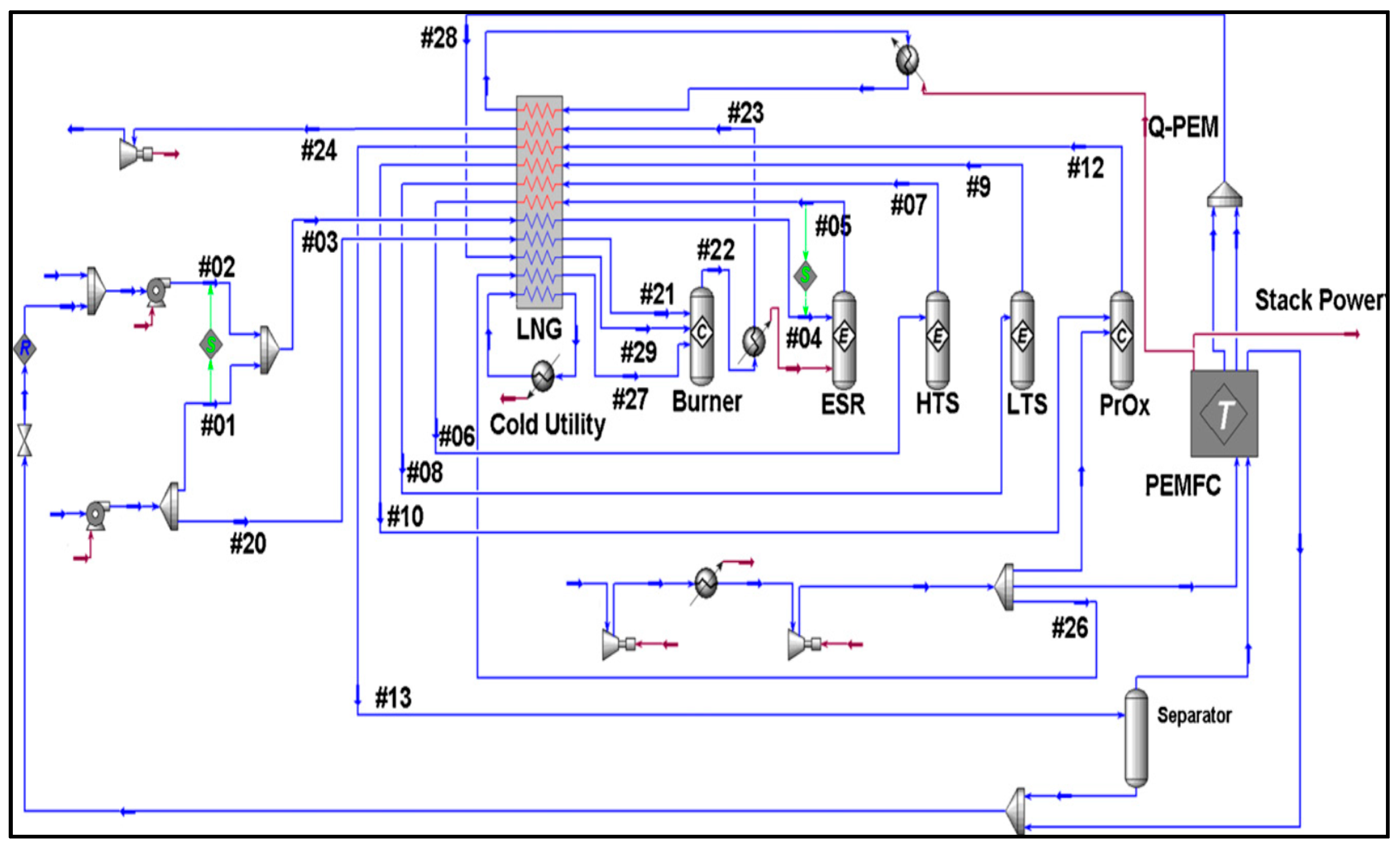
| Material Balances | ||||||||||
| Stream | 4 | 5 | 7 | 9 | 12 | 14 | 28 | |||
| T (°C) | 709 | 709 | 539 | 237 | 406 | 80 | 80 | |||
| P (atm) | 3 | 3 | 3 | 3 | 3 | 3 | 3 | |||
| Flow (kmol/h) | 0.0367 | 0.0628 | 0.0628 | 0.0628 | 0.0658 | 0.0636 | 0.1749 | |||
| Fractions | ||||||||||
| Ethanol (mol/mol) | 0.20 | 0.00 | 0.00 | 0.00 | 0.00 | 0.00 | 0.00 | |||
| Water (mol/mol) | 0.80 | 0.28 | 0.24 | 0.17 | 0.18 | 0.15 | 0.15 | |||
| Hydrogen (mol/mol) | 0.00 | 0.49 | 0.52 | 0.59 | 0.55 | 0.57 | 0.04 | |||
| CO/CO2 (mol/mol) | 0.00 | 1.17 | 0.58 | 0.03 | 0.00 | 0.00 | 0.00 | |||
| O2 (mol/mol) | 0.00 | 0.00 | 0.00 | 0.00 | 0.00 | 0.00 | 0.08 | |||
| Energy Balances | ||||||||||
| Parameter | Cold Streams | Cold Utility | Hot Streams | Reformer | Fuel Cell | |||||
| Lower T (°C) | 25–142 | 20 | 80–810 | 709 | 55 | |||||
| Higher T (°C) | 126–709 | 25 | 406–1035 | 709 | 65 | |||||
| Duty (kW) | 1.47 | 1.07 | 1.88 | 0.41 | 1.06 | |||||
| Parameter | FC T = 200 °C | FC T = 180 °C | FC T = 160 °C |
|---|---|---|---|
| Output ΔV/desired ΔV (V/V) | 0.55 | 0.55 | 0.55 |
| Current density (A/cm2) | 0.5 | 0.37 | 0.2 |
| Current drawn (A) | 208 | 153 | 83.2 |
| Electric power (kW) | 5 | 3.7 | 1.99 |
| Overall efficiency | 0.45 | 0.33 | 0.18 |
| Unit Output | T (°C) Measured | H2 (Vol/Vol %) | CO/CO2 (Vol/Vol %) | CH4 (Vol/Vol %) | |||
|---|---|---|---|---|---|---|---|
| Measured | Simulated | Measured | Simulated | Measured | Simulated | ||
| ATR reactor | 745 | 37.6 | 38.8 | 2.00 | 1.71 | 0.13 | 0.01 |
| WGS stage 1 | 400 | 41.5 | 42.9 | 19.8 | 11.5 | 0.13 | 0.01 |
| WGS stage 2 | 290 | 41.9 | 43.5 | 93.18 | 41 | 0.13 | 0.01 |
| MR reactor | 220 | 40.8 | 42.6 | - | - | 0.67 | 0.52 |
| Process Data | Steam Reforming Fractions (Vol/Vol %) | ATR Fractions (Vol/Vol %) | ||
|---|---|---|---|---|
| Species | Ethanol | Biodiesel | Ethanol | Biodiesel |
| H2 | 54.1 | 56.8 | 29.6 | 30.5 |
| H2O | 27.7 | 22.9 | 24.3 | 19.6 |
| CO/CO2 | 0.022 | 0.025 | 0.013 | 0.018 |
| N2 | - | - | 30.3 | 32.5 |
| Parameter | Steam Reforming | Electrical Reforming |
|---|---|---|
| Hydrogen Yield (kg/kg EtOH) | 0.03 | 0.044 |
| Overall Energy Input (kWh/kg H2) | 33 | 28 |
| Catalyst | a | b | ||
|---|---|---|---|---|
| Reference [45] (Ru/alumina) | 55,881 (cm3 gcat−1 h−1) | 42 (kJ/mol) | 1 | 0 |
| Reference [46] (Ni/MgO/Al2O) | 439 (mol min−1 gcat−1 atm−3.42) | 23 (kJ/mol) | 0.711 | 2.71 |
| Reference [47] (Ni/alumina) | 0.031 (mol gcat−1 s−1) | 4.41 (kJ/mol) | 0.43 | 0 |
| Temperature (°C) | 500 | 550 | 600 | |||
|---|---|---|---|---|---|---|
| Yield (mol/mol Ethanol) | Measured | Equilibrium | Measured | Equilibrium | Measured | Equilibrium |
| H2O | 4.00 | 2.99 | 4.00 | 2.68 | 2.36 | 2.41 |
| H2 | 1.56 | 2.15 | 1.85 | 2.96 | 3.63 | 3.78 |
| CO/CO2 | 0.64 | 0.25 | 0.61 | 0.32 | 0.48 | 0.62 |
| CH4 | 0.21 | 0.93 | 0.28 | 0.68 | 0.50 | 0.39 |
| C2H4 | 0.025 | 0.000 | 0.015 | 0.000 | 0.000 | 0.000 |
| RDS | Ea (J/mol) | MSE |
|---|---|---|
| 2 | 4430 | 6.0% |
| 3 | 3550 | 10.6% |
| RDS | K (mol kgcat−1 s−1) | Ea (kJ/mol) | Species | K (kPa−1) | ∆H (kJ/mol) |
|---|---|---|---|---|---|
| 1 | 11 ± 1 | 85 ± 14 | ethanol | 25 | n.a. |
| 2 | 9 ± 0.01 | 32 ± 15 | water | 3 × 10⁻⁴ | −55 |
| 3 | 23 ± 5 | 66 ± 29 | CO2 | 2 × 10⁻³ | −67 |
| 4 | 20 | 109 ± 19 | CO | 1 | −80 |
| H2 | 0.01 | −110 | |||
| Reference | [52] | [53] | [54] | [55] |
|---|---|---|---|---|
| Cat | Ni/Alumina | Ni(II)/Al(III) | Rh/MgAl2O4/Al2O3 | Co/Al2O3 |
| K1 | - | 3.06 × 10⁻⁷ (mol mgcat−1 min−1) | - | - |
| K2 | - | 1.13 × 10⁻⁷ (mol mgcat−1 min−1) | - | 4.46 × 10¹⁹ (m2 mol−1 s−1) (**) |
| K3 | - | - | - | 1.16 × 10²⁰ (m2 mol−1 s−1) (**) |
| K4 | - | 9.12 × 10⁻⁴ (mol mgcat−1 min−1) (*) | - | 4.64 × 10¹⁶ (m2 mol−1 s−1) (**) |
| Ea1 | 235.06 (kJ/mol) | 195.5 (kJ/mol) | 418 (kJ/mol) | - |
| Ea2 | 278.74 (kJ/mol) | 122.9 (kJ/mol) | 85.9 (kJ/mol) | 71.3 (kJ/mol) |
| Ea3 | - | - | - | 82.7 (kJ/mol) |
| Ea4 | - | 166.3 (kJ/mol) (*) | 107 (kJ/mol) | 43.6 (kJ/mol) |
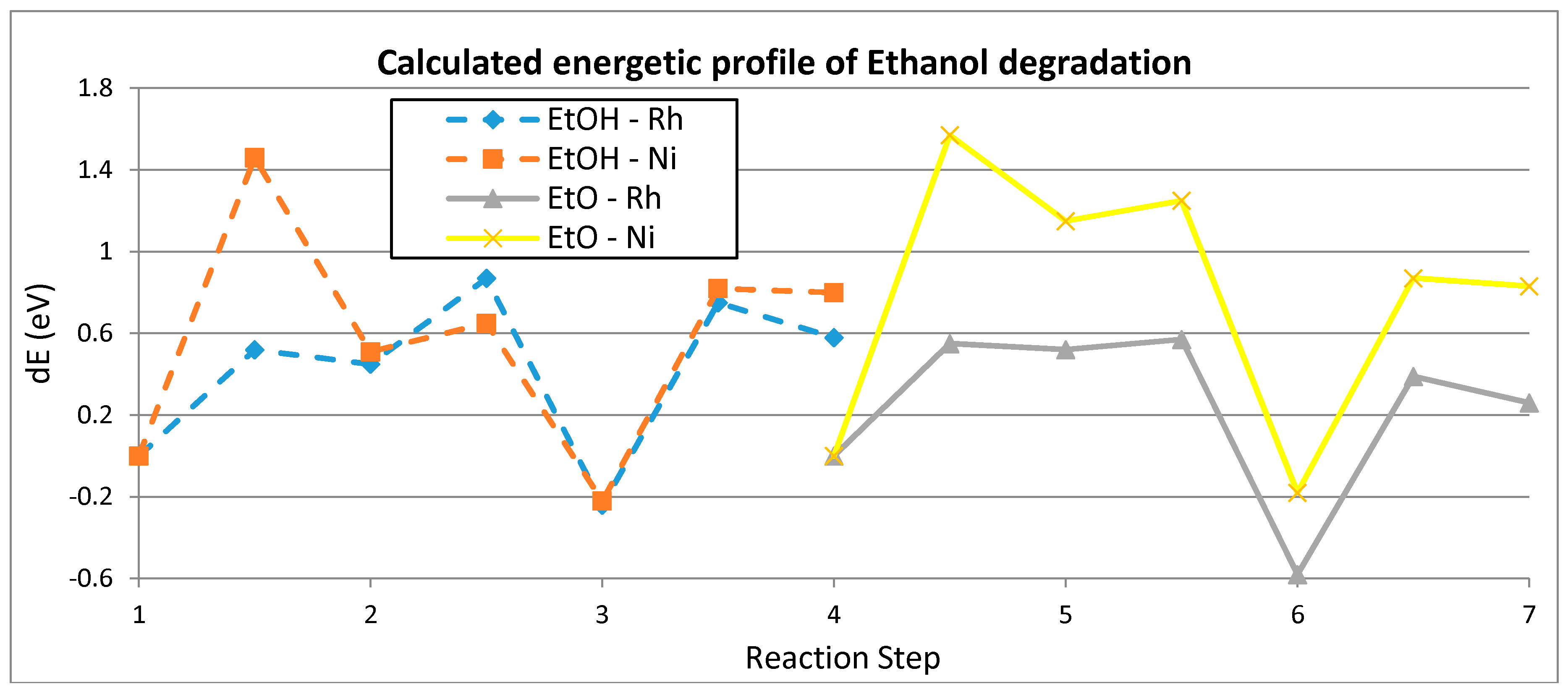
| Step | Rh | Ni |
|---|---|---|
| (1) | 0.52/0.45 | 1.46/0.51 |
| (2) | 0.42/−0.69 | 0.14/−0.73 |
| (3) | 0.99/0.82 | 1.04/1.02 |
| (4) | 0.55/0.52 | 1.57/1.15 |
| (5) | 0.05/−1.10 | 0.10/−1.33 |
| (6) | 0.97/0.84 | 1.05/1.01 |
| Catalyst | H–ZSM–5 | Cu–ZSM–5 | Ag–ZSM–5 | Au–ZSM–5 |
|---|---|---|---|---|
| kcal/mol | 43.86 | 52.75 | 40.1 | 36.29 |
| kcal/mol | 4.76 | 4.76 | 4.76 | 4.76 |
| Transition States | Computational Method 1 | Computational Method 2 | ||
|---|---|---|---|---|
| Intermediate | ∆E | ∆G | ∆E | ∆G |
| TS 1 (mechanism 3) | 50.2 ± 4.2 | 46.2 ± 4.0 | 50.2 ± 3.3 | 46.0 ± 3.3 |
| TS 2 (mechanism 4) | 54.3 ± 7.0 | 51.7 ± 6.7 | 54.9 ± 2.9 | 52.2 ± 3.3 |
| TS 3 (mechanism 4) | 53.7 ± 5.7 | 49.5 ± 5.7 | 51.0 ± 5.0 | 46.9 ± 4.8 |
| Elementary Step | (Calculation) | (Adjusted) | |
|---|---|---|---|
| −12 | 2 | 2 | |
| −7 | 28 | 24 | |
| −16 | 21 | 17 | |
| −16 | 25 | 29 | |
| −4 | 58 | 58 | |
| −9 | 29 | 29 |
| Elementary Step | Ea (kJ/mol) | A | Keq @ 500 K | Notes | |
|---|---|---|---|---|---|
| (1) | - | - | 1.1 × 10⁴ | equilibrium | |
| (2) | - | - | 8.0 × 10⁻² | equilibrium | |
| (3) | 118 | 4.0 × 10¹³ | 3.8 × 10⁻¹ | RDS | |
| (4) | 106 | 9.4 × 10¹² | 3.5 × 10⁻² | RDS | |
| (5) | - | - | 1.4 | equilibrium | |
| (6) | - | - | 7.6 × 10 | equilibrium | |
| (7) | - | - | 4.5 × 10⁻⁴ | equilibrium | |
| (8) | 92 | 3.5 × 10¹² | 7.2 × 10⁴ | RDS | |
| (9) | - | - | 1.3 × 10⁻⁶ | equilibrium | |
© 2017 by the authors. Licensee MDPI, Basel, Switzerland. This article is an open access article distributed under the terms and conditions of the Creative Commons Attribution (CC BY) license (http://creativecommons.org/licenses/by/4.0/).
Share and Cite
Tripodi, A.; Compagnoni, M.; Martinazzo, R.; Ramis, G.; Rossetti, I. Process Simulation for the Design and Scale Up of Heterogeneous Catalytic Process: Kinetic Modelling Issues. Catalysts 2017, 7, 159. https://doi.org/10.3390/catal7050159
Tripodi A, Compagnoni M, Martinazzo R, Ramis G, Rossetti I. Process Simulation for the Design and Scale Up of Heterogeneous Catalytic Process: Kinetic Modelling Issues. Catalysts. 2017; 7(5):159. https://doi.org/10.3390/catal7050159
Chicago/Turabian StyleTripodi, Antonio, Matteo Compagnoni, Rocco Martinazzo, Gianguido Ramis, and Ilenia Rossetti. 2017. "Process Simulation for the Design and Scale Up of Heterogeneous Catalytic Process: Kinetic Modelling Issues" Catalysts 7, no. 5: 159. https://doi.org/10.3390/catal7050159
APA StyleTripodi, A., Compagnoni, M., Martinazzo, R., Ramis, G., & Rossetti, I. (2017). Process Simulation for the Design and Scale Up of Heterogeneous Catalytic Process: Kinetic Modelling Issues. Catalysts, 7(5), 159. https://doi.org/10.3390/catal7050159